Report describing spatial ecosystem models

WP 4

Deliverable 4.2

Report describing spatial ecosystem models Linking habitats to functional biodiversity and modelling connectivity between regional seas Deliverable 4.2 Dissemination level

PUBLIC

LEAD CONTRACTOR Cefas

AUTHORS Christopher Lynam (Cefas), Fernando Tempera (JRC), Heliana Teixeira (JRC), Markus Diesing (Cefas), David Stephens (Cefas), Sonja van Leeuwen (Cefas), James Strong (UHULL), Lucas Mander (UHULL), Ibon Galparsoro (AZTI), Marika Galanidi (DEU), Gokhan Kaboglu (DEU), Helena Veríssimo (IMAR), Olivier Beauchard (NIOZ), Axel G. Rossberg (Cefas), Paul Somerfield (PML), João Carlos Marques (IMAR), Guillem Chust (AZTI), Ernesto Villarino (AZTI), Ángel Borja (AZTI), Anne Chenuil (CNRS), Xabier Irigoien (KAUST), Antonio Bode (IEO), María L. Fernandez (IEO), Eider Andonegi (AZTI), Ana Queiros (PML), Christian Wilson (OceanDTM), Steve Mackinson (Cefas), Stelios Katsanevakis (JRC), Vladimir E. Kostylev (Geological Survey of Canada (Atlantic)), J. Germán-Rodríguez (AZTI), Marta Pascual (AZTI), Iñigo Muxika (AZTI), Ernesto Villarino (AZTI), Xabier Irigoien (KAUST), Nihayet Bizsel (DEU), Antonio Bode (IEO), Cecilie Broms (IMR), Jacob Carstensen (AU), Simon Claus (VLIZ), María L. Fernández de Puelles (IEO), Serena Fonda-Umani (UNITS), Galice Hoarau (UiN), Maria Grazia Mazzocchi (SZN), Patricija Mozetič (NIB), Leen Vandepitte (VLIZ), Soultana Zervoudaki (HCMR), Peter M.J. Herman (NIOZ), Paul Tett (SAMS), David Mills (Cefas), Johan van der Molen (Cefas), Camilla Sguotti (ISPRA), Bernardo García Carreras (Cefas), Jim Ellis (Cefas), Georg Engelhard (Cefas), Samuele Tecchio (CNRS) and Nathalie Niquil (CNRS).

SUBMISSION DATE 31 | August | 2015

2

Contents 1.

Executive Summary .............................................................................................................................. 1 1.1. 1.2.

2.

Habitat and biological community for selected pilot areas.................................................................. 7 2.1. 2.2. 2.3. 2.4. 2.5. 2.6. 2.7. 2.8. 2.9. 2.10.

3.

Context and objectives .............................................................................................................................. 2 Main findings and outputs ......................................................................................................................... 3

Predicting areas vulnerable to invasion in the Mediterranean Sea ........................................................... 7 Multi-species modelling of polychaete assemblages in the Eastern Aegean Sea .................................... 10 Relevant spatial scales for indicators of fish and elasmobranchs in the North Sea ................................. 14 Spatial patterns in benthic biodiversity in the North Sea ........................................................................ 17 Habitat modelling of elasmobranchs in the southern North Sea ............................................................ 19 The spatial distribution of three common seabird species in the southern North Sea ........................... 23 Seabed habitats of the Greater North Sea ............................................................................................... 26 Ecohydrodynamic zones in the Greater North Sea .................................................................................. 29 EwE and Ecospace model of the North Sea ............................................................................................. 31 EwE and Ecospace model of the Bay of Biscay ........................................................................................ 34

Functional diversity within regional seas and connectivity across seas ............................................. 35 3.1. 3.2. 3.3.

Biological traits analysis and relevant spatial scales ................................................................................ 35 Process-Driven Characterization of Sedimentary Habitats within the Basque continental shelf ............ 42 Modelling of marine connectivity and biodiversity across regional seas ................................................ 45

4.

Publications resulting from D4.2 ........................................................................................................ 49

5.

References .......................................................................................................................................... 50

List of annexes Annex 1 - Predicting areas vulnerable to invasion in the Mediterranean Sea Annex 2 - Eastern Aegean Multispecies habitats Annex 3 - Indicators spatial scales North Sea Annex 4 - Seabird distributions in the North Sea Annex 5 - Seabed sediment composition in the North Sea Annex 6 - Ecohydrodynamic zones North Sea Annex 7 - Ecospace model of the North Sea Annex 8 - Ecospace model of the Bay of Biscay Annex 9 - Connectivity between seas

Supporting DEVOTES milestone reports Milestone 15 Habitat suitability models developed (30 April 2014) Milestone 16 Pilot area habitats linked to biological data for wider communities (30 June 2015) Milestone 17 Fuzzy Analysis Complete (30 June 2015) Milestone 18 Indices computed for each area (31 October 2014) Available here: http://www.devotes-project.eu/deliverables-and-milestones/

1. Executive Summary We have developed a ‘model toolbox’ to increase our understanding of the underlying processes linking species and communities to habitats and which affect the biodiversity of ecosystems. The evidence base, which this knowledge contributes to, supports the implementation of the Marine Strategy Framework Directive (MSFD) and the first assessment of Good Environmental Status (GES). Great progress has been made in recent years developing the technical specifications for indicators of biodiversity, non-indigenous species, food webs and sea-floor integrity through Regional Sea Conventions (e.g. in particular HELCOM and OSPAR) and by Member States independently. Assessments based on such indicators are required at multiple levels: ecosystem, habitats (including their associated communities) and species. The spatial scale of these assessments must be ecologically meaningful and relevant to the pressures on the ecosystem. We seek here to investigate the fundamental linkages between marine communities, habitats and state indicators that, together, provide the evidence required to determine what spatial scale is ecologically meaningful and relevant. This deliverable report is structured with respect to the following objectives of the project: -

Specific Objective 4.2: Model habitat and biological community for selected pilot areas (Section 2)

-

Specific Objective 4.3: Modelling of functional diversity within regional seas and connectivity across seas (Section 3).

A suite of studies have been pursued across regional seas to deliver these objectives and provide useful outputs to a range of stakeholders (scientists, managers and policy makers, Table 1). Some of these tasks have aimed to provide timely advice to support the implementation of this round of the MSFD (Sections 2.1, 2.2 and 2.3), while others have aimed to further the evidence base to support additional indicators in the next round of assessments (Sections 2.4, 2.5, 2.6). With focus on a longer term, we have developed data products (Sections 2.7 and 2.8) that can support the development of spatial food web models (for example see Section 2.9 and 2.10) which help us to understand the mechanisms linking pressures to states and ultimately linking management measures through the food web to change in indicators of biodiversity (see the temporal study, Lynam and Mackinson 2015). To better understand how to characterise the benthic system and integrate this functional diversity in spatial models that account for seabed habitats within regional seas, we have conducted extensive studies using Biological Trait Analyses (see Milestones 16, 17 and Section 3.1 and 3.2 of this report). At larger scales, we investigated the connectivity in biodiversity between regional seas (Section 3.3) and demonstrate that for example, the phytoplankton community can be considered to form a single group in the north-east

1

DEVOTES Deliverable 4.2

Report describing spatial ecosystem models

Atlantic, while the macrobenthos is split between Norwegian waters (Norwegian Sea, Barents Sea and northern North Sea) and the temperate waters (including southern North Sea and Celtic Seas).

1.1.

Context and objectives

This report builds on a subset of models described within DEVOTES Deliverable 4.1 “Available models for biodiversity and needs for development” and will contribute to Deliverable 4.3 “Reference levels for indicators of biodiversity for selected pilot areas”. A gap analysis reported in Deliverable 4.1 noted that models concerning non‐indigenous species (Descriptor 2) and also linking biological processes to seafloor integrity (Descriptor 6) were lacking, In response to the finding that “D2 is currently poorly addressed by the models” and “the variety of model types currently applied to non‐indigenous species is low and predominantly focuses on hydrodynamic models”, we developed and test a model framework in which we extend the potential of the Cumulative Impact index for invasive alien species to allow forecasting of areas with higher probability of future invasions (Section 2.1 and Annex 1). Similarly, Deliverable 4.1 reported that “Most models addressing D6 (seafloor integrity) lacked indicators regarding biogenic substrate or the seabed extent” and we show that this gap can be addressed using Biological Traits Analyses (see “Response and effect typologies” Section 3.1 or a “Process-Driven Characterization of Sedimentary Habitats” Section 3.2). This report demonstrates further that benthos can be linked to the environment and pressures, through multi-species modelling (Section 2.2, Annex 2). For the North Sea, Deliverable 4.1 noted that “The wide variety of benthic habitats in the North Sea was found to be poorly represented in the models … the ultimate resolution of spatial models is constrained by the information available on the seabed and benthic communities.”. The variety of habitats was investigated for patterns in benthic biodiversity (Section 2.4) and modelled relative to the distribution of elasmobranchs (Section 2.5). It was also noted that seabirds were included in the models available (SMS and EwE) as predatory groups only. However, given the importance of foraging on fish by marine seabirds it was suggested that “models that include the fish community should be more spatially resolved in order to represent the foraging range of higher predators”. To develop food web models along this path, we conducted a statistical study linking the distribution of seabirds to the abundance of their prey (Section 2.6). These developments in our scientific understanding along with new data products on substrate composition (Section 2.7, Annex 5) and on stratification regimes (Section 2.8, Annex 6) can now be used to improve the spatial food web models (Section 2.9 and 2.10, Annexes 7 and 8). This will further our understanding of the interactions between ecosystem components (and 2

indicators thereof) such that more reliable advice can be given to managers on the likely impact of particular measures aimed at maintaining biological diversity.

1.2.

Main findings and outputs

A full overview of the work conducted is given in Sections 2 and 3 and further detailed in the supporting annexes and publications arising from the work (Section 4). Outputs can be found in a repository for spatial data: http://maps.devotes.eu/ which can be navigated to from http://www.devotesproject.eu/software-and-tools/ and this will be updated as data become available. Here we summarise the progress made by each study: Table 1. Key findings and relevant audience for studies reported in DEVOTES D4.2

Study

Purpose

Target audience

Key Finding

Predicting areas vulnerable to invasion in the Mediterranean Sea

Develop a tool that can be used to effectively support prioritization of management measures to prevent invasions of alien species

EC

Model framework vulnerability mapping.

Multi-species modelling of polychaete assemblages in the Eastern Aegean Sea

Develop predictive ability for soft-sediment benthic species linked to habitats and pressures

Barcelona Convention

Tool can provide valuable information for the design of monitoring strategy and assessment of GES.

Relevant spatial scales for indicators of fish and elasmobranchs in the North Sea

To demonstrate that sub-divisions are required within the Greater North Sea region for fish biodiversity indicators

OSPAR

The study has shown that strong spatial patterns exist in the data due to the differing communities present in subregions.

Spatial patterns in benthic biodiversity in the North Sea

Identify benthic metacommunities from species data and determine local changes in biodiversity.

OSPAR

Habitat modelling elasmobranchs in southern North Sea

Identify how the spatial pattern of species has changed over the long term

OSPAR

of the

Barcelona Convention

developed

for

Scientific community

The Large Fish Indicator will need to be adapted spatially, but this will produce a better indicator more suitable to assessment and subsequent management.



Meta-community clusters were found, which can be linked to pressure maps to evaluate risk of impacts on the benthic system Occurrence of larger, less productive species (Raja clavata, Galeorhinus galeus and Squalus acanthias) declined and the largest species Dipturus batis disappeared from the area. 3



Increases were found in more resilient species of limited commercial value: Amblyraja radiata, Raja montagui, Scyliorhinus canicula, Mustelus spp. The spatial distribution of three common seabird species in the southern North Sea

Model the spatial distributions of Uria aalge, Rissa tridactyla and Fulmarus glacialis with respect to their environment (including prey) and fishing activity

OSPAR Scientific community

This study supports the use of foraging range of seabirds as a foodweb indicator The spatial distribution of prey (fish) was found to be an important factor explaining the distribution of seabirds (especially guillemots and kittiwakes) Fishing activity was not important

Seabed habitats of the Greater North Sea

Ecohydrodynamic zones in the Greater North Sea

Predict substrate composition across a large area of seabed using legacy grain-size data and environmental predictors

OSPAR

Identify stratification regimes within the North Sea that characterise the pelagic habitat

OSPAR


Quantitative estimates of the sediment composition (fractions of mud, sand and gravel) were made for the North Sea. The model-derived dataset is useful for ecological studies, where the use of broadscale categories is inadequate.


Five temporally stable ecohydrodynamic regimes were identified: permanently stratified, seasonally stratified, intermittently stratified, permanently mixed, and a Region Of Freshwater Influence. In areas with prolonged stratification the food web is diatom-based. In areas experiencing short-lived or no stratification, the base of the food web is Phaeocystis-dominated

Ecopath with Ecosim (EwE) and Ecospace modelling of the North Sea and the Bay of Biscay

Develop and evaluate the use of Ecospace models to predict and forecast changes in indicators of biodiversity and food webs


The North Sea model was able to replicate time-series of indicators from observations well. Although significant, the spatial correlation between surveys and model output was poor. More development integrating Seabed habitats and Ecohydrodynamic zones would improve the model. The Bay of Biscay model has shown promising preliminary results, but requires further development.

Biological Traits Analysis (BTA) and relevant spatial scales

Explore the applicability and relevance of BTA for indicator assessments of GES

OSPAR HELCOM Barcelona Convention Scientific

4

In the North Sea, four typological groups of benthic macroinvertebrates were found as potential ecological indicators for biodiversity and seafloor integrity. The study demonstrate a novel and comprehensive perspective of the

community

sensitivity of the North Sea seafloor invertebrate communities to physical pressure (beam-trawling) Modelled habitat classes, linked to environmental variables, reflected a range of structural and functional characteristics of the benthos.

Process-Driven Characterization of Sedimentary Habitats within the Basque continental shelf

Evaluate the ability of the model approach (mapping environmental factors influencing softbottom macrobenthic community structure and biological traits of species) to inform assessments of GES in relation to biodiversity and seafloor integrity

OSPAR

Modelling of connectivity biodiversity regional seas

Assess biological connectivity at genetic and community levels in marine species with different dispersal strategies in benthic and pelagic habitats (i.e. macro-zoobenthos and plankton)


1.3.

marine and across


Human pressures also altered benthic community structure anomalies

Similarity in population genetics and in community composition decreased with geographic distance and the rate of decline is associated to dispersal limitation. Clustering of phytoplankton and macrozoobenthos community composition data indicated the phytoplankton community can be considered to form a single group in the north-east Atlantic, while the macrobenthos is split between Norwegian waters (Norwegian Sea, Barents Sea and northern North Sea) and the temperate waters (including southern North Sea and Celtic Seas).

Conclusions and recommendations

DEVOTES have contributed innovative modelling tools (Sections 2.1 and 2.2) to fill the gap identified in DEVOTES Deliverable 4.1 for MSFD Descriptors 2 (non-indigenous species) and 6 (seafloor integrity). The project has shown that Biological Trait Analyses (Sections 3.1 and 3.2) can be used to inform Descriptor 1 (biodiversity) for benthic communities and demonstrated the importance of specific seafloor habitats to community composition and functioning. Furthermore DEVOTES has shown that such benthic communities respond to pressures in both the North Sea and Bay of Biscay (Basque continental shelf). For the first time, DEVOTES has identified the spatial connectivity in community composition and genetic similarity of macrobenthos and plankton across regional seas. A body of work focused on the North Sea (Sections 2.3 to 2.8) has developed our understanding of the factors structuring ecosystem components spatially (benthos, fish, elasmobranchs, seabirds, pelagic habitats and seafloor integrity). This knowledge will be used as the evidence to assess GES at 5



ecologically relevant scales (e.g. Section 2.3) and support future model development (particularly Sections 2.9 and 3.1) linking habitats and ecosystem components to pressures. We recommend that assessments of GES are supported by modelling studies, so that linkages between descriptors are more fully understood and ultimately targets can be set in a coherent manner. In this way, appropriate measures to manage pressures can be more easily identified. Improvements to monitoring strategies to accommodate the indicators required for the MSFD should aim to improve the availability of benthic data in particular, which will support future indicator and model development.

6

2. Habitat and biological community for selected pilot areas 2.1.

Predicting areas vulnerable to invasion in the Mediterranean Sea

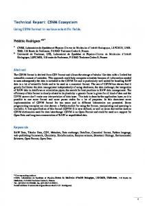
(Authors: Heliana Teixeira, Fernando Tempera, Stelios Katsanevakis) In line with the Convention on Biological Diversity (CBD) targets and recent European regulation on Invasive Alien Species (IAS), the European Marine Strategy (EU MSFD 2008) aims to acknowledge the consequences of pressures arising from non-indigenous species, through measurements of their impacts on the natural systems. For the marine domain, a recent inventory on existing biodiversity-related indicators (Berg et al., 2015; http://www.devotes-project.eu/devotool) revealed that only one indicator was available to address the ‘environmental impact of invasive non-indigenous species’ in the European seas, the ‘Biopollution level index’ (Olenin et al., 2007; Zaiko et al., 2011). A recently developed ‘Cumulative Impact index for invasive alien species’ (CIias) (Katsanevakis et al., in review) aims similarly to identify marine areas most affected by high-impact invasive alien species and help prioritize actions. By accounting for the cumulative impacts of multiple species in local and regional biodiversity, rather than just the presence of species, and by adding a spatially explicit dimension to the index output, it significantly contributes to fulfil a gap in the operational indicators set of the MSFD and efficiently address Aichi Target 9. Ecological niche modelling (ENM) has been applied successfully for evaluating the invasive potential of species (Peterson 2003; Peterson et al., 2005, 2008; Soberón and Peterson 2005). Hence we have extended the potential of the CIias (Katasnevakis et al., in review) by coupling the index with modelderived data to allow forecasting areas with higher probability of future invasions. We identified vulnerable areas to invasions based on: a) the ENM predictions of habitat suitability for potential occurrence of IAS, and b) their associated impacts on biodiversity, as measured through the cumulative impact index (CIias). The predictive nature of ENM confers a key property to an index for integrating early-warning systems (Thuiller et al., 2005; Peterson 2006), while the CIias vulnerability maps would bring obvious advantages in the context of environmental conservation programs and management of biological invasions. Our goal was to understand the capability and adequacy of ‘ready-to-use’ models in the context of wide scale conservation policy, namely for feeding specific indicators within early-warning systems. The predictions given by models developed for species native ranges were tested against known occurrences data from the invaded area. The species current occurrences and their potential distribution where then used to calculate an index of the cumulative impact (CIias) of IAS on biodiversity. The forecast of the most vulnerable areas to future invasions in the Mediterranean were compared with the currently most impacted spots at the invaded area for those IAS for which ENM models were available. In the CIias 7



index the measure of the impact of a species in biodiversity is anchored on habitat categories. Therefore we evaluated the influence of habitat mapping quality when building vulnerability maps of areas with higher potential for future invasions, within the western Mediterranean basin. The potential of ENM for conservation actions and prioritisation of measures is discussed taking into account the effect of models’ predictions in the variation of an indicator of the cumulative impact of IAS in biodiversity. Cumulative impact maps on biodiversity for the Mediterranean and preferential pathways of species introduction are discussed within the current environmental and socio-economic context. The cumulative impact of all high-impact invasive alien species (CIias) in the Mediterranean basin is higher than that based on a subset of 17 high-impact invasive alien species (Figure 1, A and B). As expected, both the extent of areas impacted and the magnitude of the impact changed. The reduced set of species used in this study constitutes a decrease of approximately 25% of cells with some impact observed. The map for the complete set of high-impact IAS represents the cumulative impact of 55 species instead of 60, since 5 of the species given for the Mediterranean presented zero occurrences in the EASIN dataset at the resolution used: Pseudochattonella verruculosa, Gracilaria vermiculophylla, Elminius modestus, Botrylloides violaceus and Liza hematocheila. For our exercise, the results will focus on the subset of 17 species for which AquaMaps models were available. The vulnerability map created with the CIias index based on future projections of species potential distribution (Figure 1C) shows that, for the whole the Mediterranean Sea and under the current conditions, the area likely to suffer the effects of cumulative impacts from multiple IAS may increase up to about 262% (Figure 1) with respect to the currently impacted area. This might change however depending on the baseline habitat mapping used. Both the projected impacted area and the magnitude of the impact will be affected, as shown for the western Mediterranean basin study area (Figure 1, C2 and C3). The work described above is further detailed in DEVOTES D4.2 Annex 1. Progress has also been reported in DEVOTES Milestone report 16 Pilot area habitats linked to biological data for wider communities (Section 3.1). A scientific paper has been submitted and a second is in preparation: Katsanevakis, S., Tempera, F. and Teixeira, H. (in review) Mapping the impact of alien species on marine ecosystems: the Mediterranean Sea case study. Diversity and Distributions Teixeira, H., Tempera, F. and Katsanevakis, S. (in prep) Predicting vulnerable areas to invasions in the Mediterranean Sea: coupling modelling data to the cumulative impact CIias index.Areas vulnerable to invasion in the Mediterranean Sea.

8

A

Figure 1. The cumulative impact index for invasive alien species (CIias) for the Mediterranean basin based on: the EASIN observed occurrences of 55 high-impact invasive alien species (A); the EASIN observed occurrences of a subset of 17 high-impact invasive alien species (B), and the AQUAMAPS species projections (P/A) for 17 high-impact invasive alien species (C). Details on the cumulative impact patterns for the Western Mediterranean basin based on lower (C2) and higher (C3) habitat mapping quality are also presented.

B

C

9


2.2.


Multi-species modelling of polychaete assemblages in the Eastern Aegean Sea

Authors: Marika Galanidi and Gokhan Kaboglu

Context Benthic infaunal species and communities have been extensively used to evaluate environmental quality of the marine environment. Within the MSFD, biotic elements of the benthos are addressed most commonly through Descriptor 6 (Seafloor integrity), criterion 6.2 (Condition of benthic communities). At the same time, the Directive has stipulations for addressing and assessing indicators linked with pressures in an explicitly spatial manner. At larger scales, achieving this through point sampling may be impractical or unfeasible; hence predictive methods are being increasingly employed to produce the large scale spatial data that are often required for the overall health assessment of wider marine areas. The aim of the current work was to develop statistical and spatial modelling tools that can capture the variability and predict the distribution of soft-sediment benthic polychaetes in the eastern Aegean Sea. More specifically, this study sets out to examine: 1. How the distribution of soft-sediment polychaetes is predicted by environmental parameters relevant to the benthos and 2. Whether these predicted distribution patterns change when pressure variables affecting the seabed are incorporated in the predictive model The resulting models are interpreted in light of the sensitivity/tolerance classification scheme for polychaetes as implemented in AMBI (AZTI’s Marine Biotic Index), an index widely employed in studies of Turkish (Albayrak et al., 2007; Çinar et al., 2012) and European marine waters (Muxika et al., 2007).

Data and methods The biological data consist of a matrix of polychaete presence/absence (total of 327 taxa after harmonisation of the data which was collated from different published sources) by 72 sites (Figure 2). Modelling was performed with taxa present in at least 10 stations (94 taxa). Environment and pressure data were also obtained from the literature and publically available sources. In order to visualise how multivariate environmental space is partitioned in the pilot area, Kmeans clustering was performed on a suit of environmental variables. Through Species Archetype Modelling (Leaper et al., 2014; Woolley et al., 2013; Foster et al., 2015) species were classified objectively, in an unsupervised way, into groups according to their responses to environmental and/or pressure gradients. The resulting logistic GLMs are termed Species Archetypes and may represent one or many species that have similar ecological/physiological tolerances. Modelling was performed with two sets of predictors. The first set consists of 7 “pure” environmental parameters, 10

i.e. bottom and surface temperature and salinity, depth and euphotic depth, primary productivity and backscattering coefficient. In the second set of variables 4 more parameters were added that reflect anthropogenic impacts to the marine environment, i.e. nutrients from fertiliser use, demersal destructive fishing, distance from ports and the Cumulative Impact Index for the Mediterranean (Micheli et al., 2013) as a measure of overall cumulative human impact to the marine ecosystem. Linear and quadratic terms were considered in order to increase the flexibility of the models to capture species responses (Leaper et al., 2014, Woolley et al., 2013).

Figure 2: Eastern Aegean Pilot area and sampled locations for biological data

Main findings Two models were produced: the “pure environmental” and the combined “environment and pressures” model. Under both models, three Species Archetypes were identified: Archetype 1 (SA1), including predominantly disturbance indifferent or tolerant species indicative of transitional assemblages, Archetype 2 (SA2), mostly characterised by sensitive and indifferent taxa and species associated with Posidonia oceanica meadows and Archetype 3 (SA3), representing primarily the stress tolerant and opportunistic taxa. Temperature and euphotic depth are the most important predictors of polychaete distribution according to the “pure environmental” model. In the combined model these gradients are complemented by pressure variables, significantly improving model fit and refining distribution patterns (Figure 3). Thus, widespread taxa (SA1) exhibit a strong response to fishing intensity, SA2 responds 11



negatively to nutrients’ concentration and SA3 displays a strong positive response to the Cumulative Impact Index, evidence that further supports the robustness of this index in capturing the way cumulative human impacts relate to ecosystem condition (Andersen et al., 2015). Better predictive performance was achieved for species with a restricted ecological niche (SA2 and SA3) while there was a slight improvement in predictive accuracy under the combined model.

Figure 3: Probability of occurrence of the three Species Archetypes (SA1, SA2, SA3) under the “environment+pressures” model (mENV+P)

Conclusion and recommendations Including pressure variables in polychaete species distribution modelling markedly improved model fit and, to some extent, spatial distribution of predictions and associated errors. It maintained the explanatory importance of environmental gradients, while at the same time bringing to focus responses to stress gradients (organic enrichment and physical disturbance) that underpin the way many synthetic benthic indicators of good environmental status are constructed. The grouping of species into Archetypes was generally in good agreement with the AMBI classification of benthic species along the stress tolerance gradient and with species assemblages previously reported from the area. On the other hand, pressure variables had a very small impact on the predictive performance of the models for individual species. This degree of “decoupling” between model fitting performance and predictive performance suggests that both habitat models contain a similar amount of predictive 12

information (Lauria et al., 2015) but this information is distributed in a different way spatially and across species. This calls for a careful consideration of predictor variables, areas of study and species to be modelled according to specific research and management objectives. The following improvements in the methodology and the quality and spatial coverage of the analysed data have the potential to produce a powerful tool that can provide valuable information for the design of monitoring campaigns and the assessment of good environmental status: 

The inclusion of hydrodynamic parameters, such as current speed and wave orbital velocity and sedimentary descriptors would improve modelling performance



The effect of prevalence may mask, to some degree, the strength of association of species based on shared responses. Removing the effect of the intercept from the mixing procedure is expected to improve model fit and predictive accuracy and result in an increased capability for finer discrimination of species on the basis of their ecological tolerances.



Poor representation or inadequate coverage of the full spectrum of environmental conditions as a source of model error can be remedied by complementing biological surveys with an appropriate partitioning technique of the relevant multivariate space and adjusting sampling design accordingly



Modelling efforts will greatly benefit if the scale and grain at which pressures are quantified matches that at which biological sampling is conducted, at least where large variability is expected. Producing and making available relevant resolution data and mapped products of pressures to the marine environment should be a national priority

Based on the findings of this study, determining the quantitative links and monitoring requirements of human activities that result in pressures affecting the main determinants of benthic species distribution (e.g thermal discharges and climate change affecting temperature and a number of activities that contribute to the disturbance and enrichment regimes, such as disposal, dredging, dumping at sea, fishing operations, industrial/sewage effluent, agricultural run-off, aquaculture) emerge as important managerial issues for the protection of benthic marine ecosystems and their various components, functions and services. The work described above is further detailed in DEVOTES D4.2 Annex 2

13


2.3.


Relevant spatial scales for indicators of fish and elasmobranchs in the North Sea

(Author: Christopher Lynam)

Aims 

To identify ecological patterns spatially within indicators of biodiversity suggested for the first MSFD assessment of GES

Introduction The MSFD calls for indicators to be developed for assessments that represent very large areas: e.g. the Greater North Sea and Mediterranean Sea. However, the indicators must also be ecologically relevant. We aim to investigate spatial patterns within indicators of fish and elasmobranchs and consider the relevance of these patterns for assessments of Good Environmental Status. Indicator-specific sub-divisions have been suggested for the Large Fish Indicator (ICES 2015), a common indicator for OSPAR in the Greater North Sea and Celtic Seas and a core indicator for HELCOM for the Baltic Sea (Oesterwind et al., 2015). So, we examine the robustness of the LFI at relativity small-scale sub-divisions.

Main findings The indicators for the demersal fish and elasmobranch community display great spatial patterns across the North Sea (Figure 4). The mean trophic level indicator of pelagic and demersal species reflects the strong north-south gradient seen in the catchrate of the bentho-piscivore guild and also the demersal to pelagic species ratio. In contrast, there is a strong east-west gradient in the size based indicators of demersal fish and elasmobranchs (shown most clearly in LFI and TyL) that appears most related to the inverse in the pattern seen in the catchrate of the benthivore guild.

14

Figure 4. Spatial patterns in indicators derived from the quarter 1 North Sea IBTS (averaged of the period 19832014), where LFI = Large Fish Index, TyL= Typical Length (cm), MML = Mean Maximum Length (MML) in cm, mean.TL = mean Trophic Level, DPR = demersal to pelagic species abundance ratio and the remaining four panels show the mean catchrate (kg per km2) of species grouped into trophic guilds (bentho-piscivores, bentivores, piscivores and planktivores).

Clearly the reduction in the size of the area used to specify the indicator can lead to extra variability due to the reduction in sample size. Our investigation of the Large Fish Indicator demonstrates that subregional assessments are required to capture the signals in the data (Figure 5), but by decreasing the size of the area covered by the indicator we increase the risk that that artefacts in the data due to smallsample size are considered as signal. However, in order to evaluate the impact of acute pressures on ecologically relevant areas a single indicator for the whole region is insufficient. A compromise must be agreed internationally concerning the appropriate size and number of sub-regions such that biological

15



assemblages are covered sufficiently, the indicator is robust to sample error and relevant to potential management.

Figure 5. Left. Partitioning of the Greater North Sea Subregion into five spatial subdivisions reflecting biological and geopolitical concerns (NW northwest North Sea; NE northeast North Sea; SW southwest North Sea; SE southeast North Sea; KS Kattegat-Skagerrak, reproduced from ICES 2015). Right, the Large Fish Indicator subset by subdivision and LOESS smoothed.

The work described above is further detailed in DEVOTES D4.2 Annex 3

16

2.4.

Spatial patterns in benthic biodiversity in the North Sea

(Author: Christian Wilson)

Aims 

Identify the underlying spatial patterns in benthic species richness

In this study we use the North Sea Benthos Survey data (Figure 6 left), a well-studied and publicly available dataset covering the entire North Sea area (see Heip 1995) to model patterns in benthic biodiversity. The most robust data that we have from any survey are the recorded species present and the location of the sample station (although there are of course taxonomic and positioning errors possible). Here we set out to extract the maximum amount of useful information from these two variables (species identity, geographic position). We do this in an explicitly spatial manner with a view to identifying spatial scales of biodiversity.

Main findings Spatial networks were constructed using innovative and novel modelling techniques to identify linkages between metacommunities from sparse sampling data and determine local changes in biodiversity. Metacommunities were identified through clustering and these clustered were then mapped out (Figure 6, right). A good degree of spatial coherence to the clusters suggesting that the approach has identified underlying patterns in community structure.

The spatial distribution traits are derived from the raw data (i.e. no inferences from other areas or other datasets are used) and are by their very nature locally adaptive. That is, the patterns are derived from the spatial distribution of the species which may behave differently in one part of the study area than they do in another (degree of clustering, frequency of occurrence). It is intended that by creating these amplified datasets we will be more able to identify spatial patters of biodiversity and demonstrate the usefulness of an explicitly spatial treatment of broadscale datasets for ecosystem monitoring purposes.

17



Figure 6. Benthos survey data (left) with stations marked by ‘x’ and with interpolated richness values. Clustering of assemblage similarity (right).

The work described above is further detailed in DEVOTES MS 16 Pilot area habitats linked to biological data for wider communities (Section 3.5)

18

2.5.

Habitat modelling of elasmobranchs in the southern North Sea

(Authors: Camilla Sguotti, Christopher Lynam, Bernardo García-Carreras, Jim Ellis and Georg Engelhard) Worldwide, shelf seas are impacted by fisheries, climate change and habitat degradation, and these pressures have been especially severe in the North Sea, with major changes in its fish community observed historically and expected for the future. Elasmobranchs are particularly vulnerable owing to large size, longevity, slow reproductive rates and associated traits (Walker and Hislop 1998; Stevens et al. 2000; Ellis et al. 2005). This study examines long-term changes in the distribution and relative abundance of the elasmobranch assemblage of the southern North Sea, based on an extensive historical time-series (1902–2013) of fishery-independent survey data.

Aims (i) document long-term changes in distribution and occurrence (‘incidence’) in surveys (ii) examine how each species’ distribution and incidence were influenced by environmental variables (including temperature, substrate and depth); and (iii) highlight the important habitats of relevance for improved management of these stocks.

Main findings Over the 112 year time-series, 2697 trawl stations with at least 10 fish species were sampled in the southern North Sea. Based on the presence/absence data for elasmobranchs at these stations, and using the environmental covariates substrate type, depth, SST and zone, we could reliably predict decadal distribution (DD) and temporal trend (TT) models for each of eight elasmobranch species; for total rays; and for total sharks (Figures 7 and 8). Common skate demonstrate a preference for rock/hard substrate, while starry ray are often found on areas that can defined as muddy to sandy mud. Lesser spotted dogfish are more likely to be found on mixed sediments while spurdog show little preference for any substrate type (Figure 9). Contrasting trends were revealed, with the larger and less productive species (thornback ray Raja clavata, tope Galeorhinus galeus and spurdog Squalus acanthias) exhibiting significant declines over the longer-term, and the largest demersal elasmobranch in the area, common skate Dipturus batis, disappearing completely from the area (last observed in 1970). In contrast, smaller species (starry ray Amblyraja radiata, spotted ray Raja montagui and lesser-spotted dogfish Scyliorhinus canicula) increased, as did smooth-hound Mustelus spp., likely benefiting from greater resilience to fishing and/or climate change. In recent years, some trends have reversed with the more northerly starry ray now declining and thornback ray increasing. This indicates a fundamental shift from historical dominance of 19



generally larger, vulnerable, but also commercially more valuable species to current prevalence of smaller, resilient species of limited commercial value. This shift may be attributed to: (1) fishing, including historical target fisheries for some elasmobranchs and the widespread increase of beam trawling in the 1960s–1970s; (2) habitat degradation, including potential degradation of outer estuarine nursery habitats and loss of biogenically-rich historical oyster beds; and (3) climate change, favouring several warm-water species. The pressures here documented to have impacted North Sea elasmobranchs over the past century are, likewise, impacting shelf seas worldwide, hence parallel changes in elasmobranch assemblages in other regions are to be expected.

20

Figure 7 Ray assemblage

Figure 8 Shark assemblage

21



Figure 7 and 8 (previous page). Spatio-temporal distribution and changes in incidence. (a) Spatial distribution in six well-sampled decades. Graded colours indicate predicted incidence (% hauls where predicted to be caught). Symbols represent the sampling stations: filled red if at least 1 ray was observed, otherwise unfilled. (b) Change in incidence (%) by pentad, 1902–2013, for the NW, E, and SW study areas (bars represent SE).

Figure 9. Substrate preference by group and species The work described above is further detailed in DEVOTES MS 16 Pilot area habitats linked to biological

data for wider communities (Section 3.3) A scientific paper has been submitted: Sguotti, C., Lynam, C., P. García-Carreras, B., Ellis, J., Engelhard, G. 112 years of changing distributions of eight skate and shark species in the North Sea (in review)

22

2.6.

The spatial distribution of three common seabird species in the southern North Sea

(Authors: James Asa Strong, Lucas Mander and Christopher Lynam) Seabirds are an important biological component of many marine ecosystems and an important element of biodiversity. Most seabird species are either predators or scavengers (Tasker and Reid, 1997). This role, combined with an estimated collective abundance in the North Sea of between 4 and 8 million individuals (Skjoldal et al., 2013), suggests that indicators derived from measurements of seabird population may represent the functioning of the food webs - this is likely to be particularly true for the birds with a colonial phase and a strong association with natural fish stocks.

Aim 

OSPAR have proposed that the reproductive success of seabirds linked to their foraging could form an indicator of food webs for the MSFD, thus to support the development of such an indicator we must understand which prey species and habitats are important to which seabird species and whether or not their foraging activity is limited by the prevailing climatic conditions.

Introduction It is estimated that almost 50 % of the collective abundance of North Sea seabirds are distributed or forage within the southern North Sea (Skjoldal et al.,, 2013) which is a pilot area considered by DEVOTES (D6.1). Multiple seabird species often congregate within one area during foraging. Synergistic foraging behaviours may allow an element of “facilitation” between species (i.e. some species may serve to improve the foraging success of other species). Once such facilitation mechanism is the attraction of seabirds to areas already occupied by other foraging birds since it is easier for seabirds to detect other foraging birds from a distance than it is to directly detect prey. Furthermore, foraging success may be enhanced within these mixed patches as differing skills between species can be combined within mixed foraging areas, e.g. surface feeding birds such as kittiwakes might be important in detecting fish and other foraging species, deep-diving birds might be more important for driving prey to the surface where they can be caught by more limited surface feeding species (Fauchald et al., 2011). These behaviours result in ‘social feeding’ which improves the foraging success for some, if not all, of seabird species present.

23



The analysis focused on three common seabird species, namely the northern fulmar (Fulmarus glacialis), common guillemot (Uria aalge) and black-legged kittiwake (Rissa tridactyla). The overall aim for this study is to establish whether the spatial foraging distribution of these species is dependent on (i) the distribution of fish species, (ii) fishing activity (as indicated by historical VMS data), (iii) the abundance of other seabird species and (iv) the physical environment (represented by bathymetry and distance to colony surfaces). Outputs from this analysis will provide (i) a more complete picture of the distribution of these species, incorporating ‘multispecies feeding associations’ (ii) a greater understanding the factors driving spatial change in the seabird distribution between years, (iii) an estimate of the spatial relationship between seabird and fish species at the scale of the southern North Sea.

Main findings Overall the statistical models for guillemots and kittiwakes were able to explain a substantial amount of the variance within the abundance associated with both species. This ability was significantly improved in models using the abundance of other seabird species as predictor variables. This was mostly driven by the underlying positive correlation between kittiwakes and guillemots. The summer guillemot models were the most successful and typically explained over 70 % of the variance. Winter models also performed well. Unlike the other two species, the winter kittiwake models out-perform the summer models. The best kittiwake model in the winter explains about 70 % of the variance. However, only about 44 % of the variance is explained by the summer kittiwake models. For the fulmar, the models (both including and excluding predictor variables using seabirds) had little predictive power for the summer or winter seasons. The fulmar is a known scavenger of bycatch from fishing activity. However, even when VMS data was included as a predictor variable, the linear regression models still failed to adequately capture the variance in the fulmar abundance. It is apparent that the majority of the predictor variables within the models were provided by the prey species for each seabird and season. It is noteworthy that when other seabird species were included as predictor variables they contributed significantly to the predictive abilities of the models. This suggests that multispecies feeding assemblages are common and detectable within the analysis. However, it is also possible that this relation between species is simply driven by the fact that they forage for the same species of fish and that their association is purely coincidental. 24

Bathymetry was highlighted as a predictor variable in almost all of the models selected. This may be related to (i) the influence depth has on the distribution of fish and hence prey for seabirds and (ii) the concentration of prey in shallow waters where a higher proportion of the fish biomass is available to foraging seabirds. Tremblay et al., (2003) observed guillemots typically diving to a depth of 10 m although dives up to 37 m were also recorded. Although the majority of the southern North Sea is less 40 m in depth, depth is nevertheless an important factor in determining whether fish are within diving range. Scheider (1997) also discusses why seabirds often correlate with depth although the examples provided operate over greater depth ranges than those considered in the southern North Sea. The work described above is further detailed in DEVOTES D4.2 Annex 4.

25


2.7.


Seabed habitats of the Greater North Sea

(Authors: Christopher Lynam, David Stephens and Markus Diesing)

Aim 

To determine whether it is possible to predict substrate composition across a large area of seabed using legacy grain-size data and environmental predictors

The seabed of the world’s oceans accounts for 71% of the surface of the Earth, harbours significant living and non-living resources, fulfils vital ecosystem services and provides a wide range of habitats for various living organisms. Yet, when it comes to accurately depicting the types of seabed substrate and habitat and the properties of the seabed for the benefits of research, resource management, conservation and spatial planning, it becomes immediately clear that there is a lack of accurate and fitfor-purpose maps and spatial models for most parts of the world’s oceans. The European Marine Observation and Data Network (EMODnet) is an attempt by the European Union to overcome such deficits in European waters. EMODnet assembles marine data, data products and metadata from diverse sources with the purpose to unlock fragmented and hidden marine data resources and to make these available. Among those data types that are being harmonised and made available are bathymetry, seabed substrates and benthic habitats.

Whilst such initiatives to unlock hidden data products and to harmonise these across national boundaries are laudable, it has become increasingly clear that this might be a challenging task. For example, EMODnet-Geology attempts to harmonise seabed substrate maps produced by geological surveys across Europe based on more than thirty differing classification schemes. The resulting classification is hence likely to be the lowest common denominator, with fairly broad classes similar to those proposed by Long (2006). In any case, maps of seabed substrate will be provided in categorical form (substrate classes) rather than as a quantity. This is somewhat unsatisfactorily, especially if one considers that sediment composition and grain size are of importance for such diverse aspects as benthic community structure (Coggan et al., 2012), Nephrops norvegicus burrow densities (Campbell et al., 2009), spatial variation in the abundance of Human Pathogen Indicator Bacteria within estuarine environments (Perkins et al., 2014), permeability in coastal marine sands (Wilson et al 2008) and compressional velocity of shelf sediments (Goff et al., 2004).

26

This study area includes the North Sea up to approximately 58.44° N and the United Kingdom’s parts of the English Channel and the Celtic Seas. The analysis combines outputs from hydrodynamic models as well as optical remote sensing data from satellite platforms and bathymetric variables, which are mainly derived from acoustic remote sensing. We make quantitative predictions of sediment composition (fractions of mud, sand and gravel) using the random forest algorithm (Figure 10). The compositional data is analysed on the additive log-ratio scale. An independent test set indicates that approximately 66% and 71% of the variability of the two log-ratio variables are explained by the predictive models. A EUNIS substrate model, derived from the predicted sediment composition, achieved an overall accuracy of 83% and a kappa coefficient of 0.60. We demonstrate that it is feasible to spatially predict the seabed sediment composition across a large area of continental shelf in a repeatable and validated way. We also highlight the potential for further improvements to the method.

27



Figure 10. Spatial plots of predicted mud, sand and gravel content.

The work described above is further detailed in DEVOTES D4.2 Annex 5 A scientific paper has been submitted: Stephens, D., and Diesing, M. (in review) Towards quantitative spatial models of seabed sediment composition. PLOS ONE 28

2.8.

Ecohydrodynamic zones in the Greater North Sea

(Authors: Sonja van Leeuwen, Paul Tett, David Mills, and Johan van der Molen)

Aim 

Identify stratification regimes within the North Sea that characterise the pelagic habitat

The Marine Strategy Framework Directive aims to limit anthropogenic influences in the marine environment. But marine ecosystems are characterized by high variability, and it is not trivial to define its natural state. Here, we use the physical environment as a basis for marine classification, as it determines the conditions in which organisms must operate to survive and thrive locally. We present a delineation of the North Sea into five distinct regimes, based on multi-decadal stratification characteristics. Results are based on a 51 year simulation of the region using the coupled hydrobiogeochemical model GETM-ERSEM-BFM. The five identified regimes are: permanently stratified, seasonally stratified, intermittently stratified, permanently mixed, and Region Of Freshwater Influence (ROFI). The areas characterized by these regimes show some interannual variation in geographical coverage, but are overall remarkable stable features within the North Sea. These regimes form spatially and temporally stable features of the North Sea hydrodynamic regime, with the core areas covering 71% of the total North Sea domain (Figure 11). The remaining 29% is characterized by large interannual variability which defies classification. These are mainly transitional areas, which can belong to different regimes in different years. The spatial stability of the identified regimes indicates that carefully selected monitoring locations can be used to represent a substantive area of the North Sea. The biological characteristics of these regimes differ from diatom-based food webs in areas with prolonged stratification to Phaeocystis-dominated food webs in areas experiencing short-lived or no stratification. Although we have made progress in showing how the floristic composition of the phytoplankton (as shown in the contribution and seasonality of each simulated lifeform) relates to physical regime, there remains much more to do both with simulations and with observations to assemble the definitive account of links between physics and biology that will correspond to the picture painted by biome theory of terrestrial environments. Nevertheless, effective marine management, such as that required by the MSFD, must take account of the existence of five ecohydrodynamic regimes in the North Sea, and their likely biological consequences, as well as acknowledging the large interannual variability in the zones between the regime cores.

29



Figure 11. Time median results of the modelled, annual regions in the North Sea based on density stratification. Transparent areas indicate areas where the dominant regime occurs for less than 50% of the time (less visible due to minimal occurrence).

The work described above is further detailed in DEVOTES D4.2 Annex 6 and the publication: van Leeuwen, S., P. Tett, D. Mills, and J. van der Molen (2015), Stratified and nonstratified areas in the North Sea: Long-term variability and biological and policy implications, J. Geophys. Res. Oceans, 120, doi:10.1002/2014JC010485. http://onlinelibrary.wiley.com/doi/10.1002/2014JC010485/full

30

2.9.

EwE and Ecospace model of the North Sea

Authors: Christopher Lynam and Steven Mackinson

Aim 

To assess the skill of existing food web models to model ecological indicators

Introduction Ecopath with Ecosim (EwE) food web models are useful tools to evaluate ecosystem impacts of both climate change and fisheries management measures (Lynam and Mackinson 2015; Piroddi et al., 2015). Here, we simulate biodiversity and food web indicators using two versions of the model of the North Sea: a temporal only model (Mackinson 2014; Mackinson and Daskalov 2007) and a spatio-temporal model (Romagnoni et al., 2015). These model derived indicators are then compared to survey data (International Bottom Trawl Survey, IBTS) to evaluate the skill of each model.

We derive a number of biodiversity and food web indicators directly from the model simulations (Figure 12). State indicators considered here are:

  



mean trophic level of demersal fish and elasmobranchs (MTL) and all surveyed species (MTLs) mean maximum length (ML) of all surveyed fish and elasmobranchs the biomass trends of key trophic guilds (Psc = Piscivores, BPs = Bentho-piscivores, Ben = benthivores, Plk = Planktivores, BIO = all demersal fish and elasmobranchs, and BIOs all surveyed fish and elasmobranchs) Large Species Indicator for demersal fish and elasmobranch species only (LSI) and for all surveyed species (LSIs)

31



Figure 12. Average spatial distribution for the period 1991-2007 for a set of ecological indicators derived from the North Sea Ecospace model (note that these maps will differ from survey derived indicators due to the differing catchabilities of species in the survey).

Main findings Indicators derived from the temporal model, Ecopath with Ecosim, of the North Sea agree well with the trends in the observed IBTS data and we have used the model to explore pressure-state relationships (Lynam and Mackinson 2015). The spatial model demonstrates the much of the fish and elasmobranch biomass in the North Sea is located along UK and European coastlines in the southern North Sea. In contrast, a north-south gradient is shown in the indicators of size structure and trophic level, with larger and high trophic levels in the northern North Sea. Although the the current parameterization of Ecospace captures some of the variability in the indicators spatially the model requires further development in order to improve its skill. The mean trophic level was best modelled by Ecospace (i.e. greatest Mantel correlation coefficient, Figure 13) while the biomass of benthivores and the mean maximum length of all surveyed fish and elasmobranchs were modelled particularly poorly.

32

Figure 13. Mean trophic level of all surveyed fish and elasmobranchs (MTLs) derived from the Ecopath with Ecosim and Ecospace (left) and computed from IBTS data (centre), showing the Mantel correlogram of the Hellingertransformed and detrended data (black squares indicate significant spatial correlation after Holm correction for multiple testing and distance classes are given in units of km). The work described above is further detailed in DEVOTES D4.2 Annex 7.

Temporal simulations are published in Lynam and Mackinson (2015) How will fisheries management measures contribute towards the attainment of good environmental status for the North Sea ecosystem? Global Ecology and Conservation 4, 160-175 doi: 10.1016/j.gecco.2015.06.005 http://dx.doi.org/10.1016/j.gecco.2015.06.005

33



2.10. EwE and Ecospace model of the Bay of Biscay Authors: Eider Andonegi, Samuele Tecchio and Nathalie Niquil

Aim 

To develop a model that can be used to assess potential changes in the dynamics of the Bay of Biscay ecosystem and account for the spatio-temporal variability of the system.

Main findings The static food web model Ecopath of the Bay of Biscay is complete but the temporal and spatial components of the EwE model are in development. The flow diagram of the balanced model is shown in Figure 14, where different functional groups are represented by a node and existing relationships are represented by an arrow. Preliminary results from temporal model (Ecosim) fitting are given in the detailed Annex 8. For the spatio-temporal model (Ecospace) data are being collated related to temperature and salinity optimums for each functional group, habitat maps of the study area along with data from the IBTS survey.

Bottlenose dolphins 5 Striped dolphins

Harbour porpoises Long-finned pilot whales Piscivorous demersal fish Common dolphins Pelagic cephalopods

Pursuit divers seabirds

Piscivorous 4 and benthivorous demersal fish Mackerel Horse mackerel

Surface feeders seabirds

Suprabenthivorous demersal fish Benthivorous demersal fish

SpratBenthic cephalopods Anchovy

Sardine Carnivorous benthic invertebrates

3

Mesozooplankton Macrozooplankton Sub-surface deposit feeders invertebrates Suprabenthic invertebrates Benthic meiofauna Necrophagous 2 benthic invertebrates Surface suspension and deposit feeders inv

1

Large phytoplankton

Small phytoplankton

Discards

Figure 14. Flow diagram of the Ecopath model of the Bay of Biscay.

This work is further detailed in Devotes 4.2 Annex 8. 34

Microzooplankton Bacteria

Detritus

3. Functional diversity within regional seas and connectivity across seas 3.1.

Biological traits analysis and relevant spatial scales

(Authors: Helena Veríssimo, Olivier Beauchard, et al.) A review on marine environment Biological Traits Analysis (BTA, Figure 15) was presented in MS17 (section 3). Gaps and shortcomings in the application of this multi-trait approach for describing functioning were identified and the state of the art updated, in order to understand the present-day applicability and relevance of this approach in the marine realm.

Figure 15. Illustration of data sets necessary to BTA; rectangles represent data matrices containing either quantitative or qualitative data; arrows indicate that tables match each other by rows or columns. A. Complete data set enabling BTA at both species and community levels; different questions can be investigated such as the relationships between environment (R) and organisms communities (L), between organisms (L) and biological traits (Q), but also between environment (R) and traits (Q). B. Matrix multiplication enabling BTA at the community level only.

Relevant spatial scales for traits in the North Sea were addressed in MS17 (section 4). Two different functional typologies are being developed in the North Sea for state (life-history) and effect (bioturbative characteristics) traits. The procedure to build the functional groups , map and relate them to environmental characteristics along the North Sea is briefly described below (section 3.1.1). To model relationships between taxonomic and functional composition MS17 (section 5) reported on two approaches: 

the performance of two indicators (M-AMBI and Rao’s Quadratic Entropy) in the Bay of Biscay is assessed and compared (section 5.1);

35





the behaviour of a number of taxonomic and functional relatedness measures was assessed at a large spatial scale using coastal macrobenthic assemblages of Bay of Biscay, North Sea and Kattegat (section 5.2, Figure 16).

Figure 16. Map of the case study areas. (Base map adapted from the European Atlas of the Seas, EC; http://ec.europa.eu/maritimeaffairs/atlas/maritime_atlas/).

The work described above is further detailed in DEVOTES Milestone 17 Fuzzy Analysis Complete and Milestone 18 Indices computed for each area

a.

3.1.1. Response and effect typologies, and identification of related spatial scales:

(Authors: Olivier Beauchard, Ana Queirós and Peter M.J. Herman)

Aim 

To derive typological groups of benthic macroinvertebrates as potential ecological indicators for Descriptor 1 (Biodiversity) and Descriptor 6 (Seafloor integrity).

The North Sea benthic macroinvertebrates were used in these studies since the biology of respective communities is the most documented among those from the different European seas (Heip et al.,, 1992). Two sets of traits are considered to infer about survival and ecosystem engineering, response and effect traits, respectively. Based on these traits, two different typologies were developed aimed to derive typological groups as potential ecological indicators in general, and more relevantly for both Descriptor 1 (Biodiversity) and Descriptor 6 (Seafloor integrity) from the MSFD.

Main findings Response traits: Main outputs of MCA on response traits are detailed in task 3.2.1 from DEVOTES WP3 (Deliverable 3.2). Briefly, four main groups were identified: 36

Group 1: tubicolous, intermediate to large body size, short to intermediate lifespan, early maturity, high reproductive resilience; Group 2: characteristics intermediate between Group 1 and Group 3; Group 3: long lifespan, late maturity, low reproductive resilience; Group 4: short body size, early maturity, continuous reproduction, large propagules. Group 1 relative density was shown to respond positively (p < 0.05) to beam-trawl fishing intensity whereas Group 2 relative density was found to respond relate negatively (p < 0.05). The relative densities of the four groups are mapped over the whole North Sea in Figure 17. These maps represent a novel and comprehensive perspective of the sensitivity of the North Sea seafloor invertebrate communities to physical pressure, especially regarding Group 2 distribution, and fit well with previous work in the region (Callaway et al., 2002; Queirós et al., 2006; Tillin et al., 2006; Reiss et al., 2010).

Figure 17. Relative response group density (%) distribution over the North Sea. Values express the proportions of individual per location (relative individual density in %).

Six main groups were identified from the analyses on effect traits: 37



The first group was mainly composed of tubicolous worms characterized by vertical conveying. Groups 2 to Group 5 were gradually positioned along the first axis. Group 2 was composed of surficial sediment mixers, represented by diverse polychaetes and bivalves; Group 3 included sub-surface mixers, mostly bivalves and ophiuroids; Group 4 was dominated by diffusors occurring at mid-depth such as phyllodocid worms, ophiuroids and spatangoids; Group 5 comprised most of regenerators (crabs) and gallery builders (callianassids); Group 6 comprised exclusively amphipods and cumaceids. Maps of effect group relative densities are shown in Figure 18. All group distributions were significantly explained by space, from 16 to 56 % of their total variance. Group 1 and Group 6 exhibited very similar patterns than response Group 1 and response Group 4 respectively, with similar spatial structures. Their distributions were explained by a few scales, from the largest ones (MEM 1 and 2, circa 1000-500 km) to smaller ones (MEM 23 to 198, circa 300-20 km). Although large scales (MEM 1 to 5) had higher contributions in all models, a larger mix of intermediate, small to very small scales explained the main part of the explained variance of Groups 2–5 distributions.

Figure 18. Relative effect group density (%) distribution over the North Sea. Values express the proportions of individual per location (relative individual density in %).

38

This points out critical seafloor functions which may be widely distributed through local spatial waves rather than lying homogeneously in large isolated zones, i.e. there may be seemingly a variety of different drivers acting simultaneously on these species, which vary at different spatial scales. Groups 2– 5 were the largest contributors to non-local sediment mixing by actively burrowing; their living modes, more spatially complex, might require more specific environmental conditions and more locally variable. Further analyses with habitat descriptors will be necessary to validate this hypothesis. These application examples provide potential indicator development for European marine environments. The use of two different typologies demonstrated some divergences and convergences among response and effect group distributions. Although some similar patterns were observed between the two typologies, spatial scales explaining distributions were markedly different, suggesting that typologies may result from different scale-dependent processes. Correlation analyses between group individual densities and environmental descriptors highlighted significant relationships (Table 2, Table 3). Although all environmental descriptors were not measured at all locations, especially bottom wave energy and water current velocity (not available above 57° North), these results support the existence of a non-random selection of group distributions by habitat conditions. Correlations with granulometric fractions and median grain size were the most contrasting among response and effect groups; effect groups were in general more specific to the nature of the substratum, supporting a higher affinity of effect traits used here which directly translate the organism affinity for sediment types. However, as highlighted by the effect trait analysis, the main characteristic distinguishing effect groups was their ability to displace the sediment, from local to distant locations, from 1D to 3D structure. Additionally, effect group distributions overlapped much more than response group due to their depth preferences. Hence, the implication of small spatial scales in their distributions, from one sampling station to another, might suggest local sediment heterogeneity. Table 2. Pearson’s correlation coefficients between response group individual densities and environmental descriptors. Values in bold indicate significant relationships at the α-level = 0.05. “CV” for coefficient of variation of monthly median values. Environmental descriptor Depth Bottom current velocity

Group 1

Group 2

Group 3

Group 4

0.48

0.03

- 0.14

- 0.25

- 0.11

- 0.30

- 0.20

0.07 - 0.04

CV bottom current velocity

0.02

0.10

0.06

Mean bottom wave energy

- 0.31

- 0.21

- 0.06

0.14

0.07

0.25

0.17

- 0.04

Mean water O2 concentration

- 0.31

- 0.04

0.00

0.22

CV water O2 concentration

- 0.35

- 0.01

0.13

0.11

0.01

0.25

0.09

- 0.41

Silt fraction

- 0.01

0.19

0.14

- 0.42

Sand fraction

- 0.19

0.14

0.18

0.28

CV bottom wave energy

Clay fraction

Median grain size

0.14

0.08

0.01

- 0.14

Sediment organic carbon content

0.15

- 0.04

0.01

0.00

39



Table 3. Pearson’s correlation coefficients between effect group individual densities and environmental descriptors. Values in bold indicate significant relationships at the α-level = 0.05. “CV” for coefficient of variation of monthly median values. Environmental descriptor

Group 1

Group 2

Group 3

Group 4

Group 5

Group 6

0.41

- 0.06

0.53

- 0.16

0.23

- 0.31

- 0.29

- 0.23

- 0.34

0.12

0.08

0.13

CV bottom current velocity

0.06

0.08

0.10

0.08

- 0.16

- 0.14

Mean bottom wave energy

- 0.29

0.01

- 0.64

0.14

- 0.49

0.17

Depth Bottom current velocity

0.13

0.27

0.29

- 0.13

0.07

- 0.05

Mean water O2 concentration

- 0.26

0.07

- 0.35

0.06

- 0.23

0.26

CV water O2 concentration

- 0.27

0.07

- 0.36

0.04

- 0.23

0.15

0.29

- 0.16

0.37

- 0.36

0.40

- 0.51

CV bottom wave energy

Clay fraction

0.25

- 0.13

0.28

- 0.37

0.39

- 0.53

- 0.27

0.25

- 0.15

0.22

0.07

0.38

Median grain size

0.34

- 0.04

0.28

- 0.35

0.04

- 0.20

Sediment organic carbon content

0.22

- 0.23

0.07

0.00

- 0.05

0.01

Silt fraction Sand fraction

Spatial scale-dependent process is an important notion to consider in ecological indication but one that is not well addressed by small monitoring programs covered by single institutes or countries. As shown here, the benthic communities of the North Sea exhibit spatial structures that vary at small as well as large scale – the present study is based on the most comprehensive dataset available for the North Sea. Results suggested that indicators based on these communities will likely require large monitoring programs; or monitoring programs focused spatially in areas identified as having different functional structures in this study. Multi-scale-dependent indicators may provide ideal tools for marine monitoring as large scale variations only may locally limit indicator relevance. Spatial scales could explained variable amounts of variance of group relative densities; some scales explained 1 % whereas some others explained 14 %. Although residual variance can account for random community structures (Dray et al., 2012), the North Sea is nevertheless intensively trawled so that naturally organized patterns have been found to have been disrupted, and community structure largely reflect trawling effort (Queirós et al., 2006; Tillin et al., 2006). Lastly, effect traits may deserve more attention. We found spatial structures in the communities that we analysed. Because bioturbation (and associated bioirrigation) directly influences important biogeochemical processes such as nutrient cycling and primary production among others (Queirós et al., 2013 for a review; Carrol et al., 2008), spatial structuring of bioturbation has a direct bearing for MSFD Descriptor 6 – Seafloor integrity – and deserves further attention in indicator development (Birchenough et al., 2012; Van Hoey et al., 2013). Other types of ecological engineering such as habitat creation (e.g. biogenic reef building, shell deposition) have not yet been considered in similar analysis (Gutiérrez et al., 2003). Future improvement of the data set should enable a better identification of 40

seafloor areas sensitive to physical pressures (e.g. beam-trawling, dredging) and ensuring important functions (i.e. ecosystem services). The work described above is further detailed in DEVOTES Milestone 17 Fuzzy Analysis Complete and Milestone 18 Indices computed for each area

41


3.2.


Process-Driven Characterization of Sedimentary Habitats within the Basque continental shelf

(Authors: Ibon Galparsoro, Ángel Borja, Vladimir E. Kostylev, J. Germán- Rodríguez, Marta Pascual and Iñigo Muxika)

Aim 

Test the applicability of a process-driven benthic sedimentary habitat model to inform assessments of GES in relation to the biodiversity and seafloor integrity descriptors for sedimentary habitats (Borja et al., 2011; Rice et al., 2010; Van Hoey et al., 2010).

The process-driven marine benthic habitat mapping approach, as proposed by Kostylev and Hannah (2007), is based upon ecological theory that relates species life-history traits to the properties of the environment (Huston, 1994; Margalef et al., 1979; Reynolds, 1999; Southwood, 1977), transforming maps of the physical environment into those of benthic habitat types (Galparsoro et al., 2013).

Data acquisition For this investigation, soft-bottom macrobentos data and a set of 16 environmental variables were considered, which could be grouped into: (i) seafloor morphology (depth and distance to rock); (ii) sediment characteristics (mean grain size, sorting, gravel content, sand content, fine content, organic matter content, redox potential) and sediment resuspension index; and (iiii) oceanographical conditions near the seafloor (average annual chlorophyll content, average spring chlorophyll content, annual mean temperature, annual temperature range and minimum annual temperature). In terms of biological data, 404 grab samples were collated. Macrobenthic species were identified at species level whenever possible (a total of 1,202 species). For each sample species richness (number of taxa) and Margalef index were determined. The species life-history traits extracted from the Life Information Network (MarLIN, 2006). Eight biological traits were selected for the analysis: lifespan; maturity; generation time; size; living habit; sociability; fragility; and flexibility (see Galparsoro et al., (2013), for further details on the detailed description of the datasets used in the analysis).

Analytical Approach The correlation between: (i) species composition and the spatial location of the samples; (ii) environmental variables and spatial location of samples; and (iii) taxon composition and environmental conditions, were analysed. The significance of any relationship between taxon composition and environmental conditions; likewise the environmental variables that best matched the distribution of taxa was investigated (Bremner et al., 2006; Clarke and Ainsworth, 1993; Louzao et al., 2010; McArthur et al., 2010; Shumchenia and King, 2010; Todd and Kostylev, 2011). Each sample was classified according to 16 classes. Finally, an analysis of similarity was carried out. Species richness and diversity (Shannon) 42

of the samples were interpolated in the process-driven habitat template to analyse the ecological significance of the template. Once classes were identified, the average similarity and the representative species for each assemblage, based upon the similarity percentages method were estimated. Finally, the traits of the species of each of the defined habitat classes were analysed (see Galparsoro et al., (2011), for further details).

Main findings The response of the benthic structural parameters - species richness and Margalef index - to the resuspension index has indicated that species richness decreases rapidly as the resuspension index increases, this lies near to the threshold of sediment resuspension. The Margalef index showed almost the same response, with an almost proportional decrease in comparison to an increase in the resuspension index.

Regarding to the species traits composition, some general patterns were observed: species with shorter lifespan (

Report describing spatial ecosystem models

Report describing spatial ecosystem models

Suggest Documents

Deliverable No. 157 Report/paper describing spatial ...

Describing the software forge ecosystem - FLOSSmole

A SPATIAL ECOSYSTEM - WCPFC

Workshop Report Describing Scientific ...

Pitch, roll, and yaw: Describing the spatial

Metadata for Describing Water Models - iEMSs

Ecosystem Effects Workgroup Report

startup ecosystem report - Squarespace

Utility of Phenomenological Models for Describing Temperature

EMPIRICAL MODELS FOR DESCRIBING FIRE BEHAVIOR IN ...

startup ecosystem report - Squarespace

linear and nonlinear-segmented models describing ...

Multivariate Spatial Process Models

NSW Annual Report Describing Adverse Events Following ...

Integrating ecosystem services into spatial planningâA spatial ... - Core

Integrating ecosystem services into spatial planningâA spatial ... - Core

Technical Report: CSVM Ecosystem - arXiv

Spatial optimisation of ecosystem services - Landcare Research

Ecosystem Services in Municipal Spatial Planning - SLU

Consequences of spatial heterogeneity for ecosystem ... - esanalysis

Aquatic Ecosystem Health & Management Spatial ...

Benthic Ecosystem Structure: Spatial and Temporal ...

Spatial characterisation of the Benguela ecosystem ...

Synergy between Ecosystem Thinking and Spatial Planning

Report describing spatial ecosystem models