Representative datasets for neural networks Rocio Gonzalez-Diaz
1,2
, Eduardo Paluzo-Hidalgo 3
Dept. Applied Math I University of Seville, Seville, Spain
Miguel A. Guti´errez-Naranjo 4 Dept. Computer Sciences and Artificial Intelligence University of Seville, Seville, Spain
Abstract Neural networks present big popularity and success in many fields. The large training time process problem is a very important task nowadays. In this paper, a new approach to get over this issue based on reducing dataset size is proposed. Two algorithms covering two different shape notions are shown and experimental results are given. Keywords: Algorithm, α-shape, proximity graph, neural networks.
1
Introduction and background
Reducing time in the training process in Machine Learning algorithms is a vivid area nowadays. It is on the basis of many current tools as the use of 1 2 3 4
Email:
[email protected] Partially supported by MINECO, FEDER/UE under grant MTM2015-67072-P. Email:
[email protected] Email:
[email protected]
Contrastive Divergence in Restricted Boltzmann Machines or even in the motivation for the use of Convolutional Neural Networks [6]. Many of the efforts have the aim of reducing the dimensionality of the data, as the classic Principal Component Analysis method [7]. In this paper, a different approach is proposed. The first key idea is that close point data provide similar information in the training process and therefore, training time can be reduced by removing some of such similar data without losing accuracy. In order to achieve such size reduction, the dataset is embedded in a metric space and a new pooling strategy based on proximity graphs density is proposed. The second key in this paper is based on the α-shape of the point cloud [1]. We show that such subset of points has vital information for training a neural net. In this paper, the Hausdorff distance is considered to measure the distance between sets in Rn with the Euclidean metric and a fully connected feedforward multilayer perceptron is used as the Machine Learning tool. Let G be an undirected graph, V (G) the set of vertices and E(G) the set of edges 5 . Let X ⊂ Rn be a point cloud, ε ∈ R and (X, d) a metric space. An ε-distance proximity graph G(X, ε) is the graph whose vertices are V (G) = X and edges E(G) = {(x, y)| x, y ∈ X , d(x, y) ≤ ε}. Let x ∈ X be a sample point. x is called α-extreme if there exists an open ball of radius 1 , B 1 , such that x lies on the boundary and B 1 contains all the points of α α α X. Finding such α-extreme uses Delaunay triangulations [3], but a detailed description goes beyond the scope of this paper. Let X, Y ⊂ Rn two nonemtpy point clouds endowed with the same metric. Hausdorff distance is defined by dH (X, Y ) = max{supx∈X infy∈Y d(x, y), supy∈Y infx∈X d(x, y)}. A neural network (NN) [5] is a massively parallel distributed processor made up of simple processing units that has a natural propensity for storing experiential knowledge and making it available for use. NNs can be described as hierarchical directed weighted graphs which nodes are called neurons. These neurons are distributed in layers. NNs receive an input which is processed across neurons by functions predefined, called activation functions, giving a numerical output. When NNs are just forward oriented and nodes between layers are fully connected, they are called fully connected feedforward NNs 6 . A neural network learning algorithm modifies NN parameters in order to optimize a cost function. Stochastic gradient descent is a NN learning algorithm that performs a parameter update following the opposite direction of the gradient. 5 6
The reader is assumed to be familiar with graph theory. For a further reading about neural networks [4].
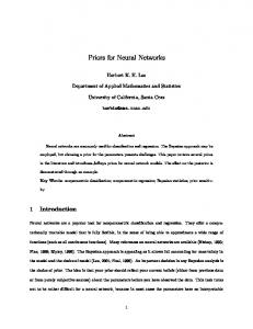
(a) Cloud of the dataset
(b) NN output
(c) NN classification
Fig. 1. Neural Networks as a surface fitting problem
2
Stating the problem
Given a dataset X ⊂ Rn × {0, . . . , k} with 0, . . . , k the classification labels, after training a neural network with X, Rn is splited in k regions according to the classification of the points. In such way, a manifold frontier of the prediction of a neural network is obtained as a process of local search, based on minimizing a given cost function (two dimension example in Fig. 1). Training such neural nets usually takes a long time, due mainly to the large amount of points of the dataset. In this paper, we wonder about the possibility of reducing the number of points of the dataset without losing accuracy. The chosen subset of significant points is called a representative subset of the dataset. The underlying idea on the selection of representative dataset is that close points provide similar information to the learning process and, in some sense, such information is redundant and therefore, some points of the dataset can be removed. This way, the remaining points keep the same information and the obtained neural nets are comparable as classification tools.
3
Algorithms for computing representative datasets
Two algorithms for obtaining representative datasets are proposed. Proximity Graph Based Algorithm (PGA) reduces the dataset size using proximity as a criterion for deleting points. Given a point cloud dataset X ⊂ Rn (e.g. Fig. 2a). A distance d ∈ R is a hyperparameter used to construct a proximity graph G(X, d) which summarizes information about density and neighborhood of X. In order to find clusters, a community detection algorithm is applied to G(X, d), encapsulating agglomeration notion in a set of communities (e.g. Fig. 2b). Finally, site percolation is performed, following any strategy as random sampling in each community or any stochastic process as deletion of high degree nodes. The result of the algorithm is a simplified
(a) Original dataset
(b) Set of communities
(c) Simplified dataset
Fig. 2. Application of the proximity graph algorithm
(a) Original (3.000 points)
dataset
(b) PGA dataset (1497 points)
(c) α-extremes dataset (867 points)
Fig. 3. Original dataset and representative datasets
version of X keeping its shape, as we see in Fig. 2c. In order to avoid getting an imbalanced dataset, the algorithm is applied for each class. The complexity of the algorithm depends on the different choices of community algorithm and sampling method. Algorithm 1 Proximity graph representative dataset (PGA) Input: Point cloud dataset X ⊂ Rn × {1 . . . k} and d ∈ R ˆ ⊂ X. Output: A point cloud X for i = 1 to k do Gi (Xi , d) where X ⊃ Xi ⊂ Rn × {i} ci = communityDetection(Gi ) ˆ i = sampling(ci ) X ˆ = Sk X ˆi X i=1
The second approach is based on the concept of α-shape. In order to capture the intuitive notion of shape, we propose α-extreme representative dataset as a sufficient dataset for a neural network. An efficient algorithm to obtain α-shapes was firstly introduced in [3]. These α-shapes can be obtained with a O(n · log n) algorithm with O(n) space in two dimensions and with k−1 O(n| 2 | ) space in k dimensions. To compute α-extremes, firstly Delaunay triangulation is determined and after that, α-extremes are easily obtained. Algorithm 2 α-extreme representative dataset Input: Point cloud dataset X ⊂ Rn × {1 . . . k} ˆ ⊂ X. Output: A point cloud X do Compute α-shapes (e.g. alphahull R package) ˆ = α-extremes X
4
Experiments
In this section, some experimental results are presented using proximity graph based algorithm and α-extremes subset. A fully connected feedforward neural network was used. It has 100 neurons in the unique hidden layer, hyperbolic tangent activation function and softmax output activation function. It was trained with stochastic gradient descent with mini batch size 50, 100 epoch iterations and momentum parameter 0.9. This neural network was trained with three different datasets: an original dataset, a simplified version of the original (which is output of the PGA) and the α-extreme dataset. Fig. 3 shows these datasets. Hausdorff distance between the original dataset and graph based algorithm output dataset is 0.3227921 and, Hausdorff distance between the original dataset and α-extremes dataset is 0.6030393. Furthermore, mean square error is 0.16 for each neural network predicting over the original dataset. Accuracy predicting, i.e. percentage of well classified points, over the original dataset is, for the three neural networks, on the range (95 − 96%).
5
Conclusions and Future Work
Reducing dataset size can be a nice approach in order to understand NNs stability and functionality. We have shown two representative datasets styles that cover different shape notions. Furthermore, we also show that NNs can do nice predictions using simplified datasets. Future work would consist on: (1) formalizing that representative datasets can be a good strategy to achieve optimization and accuracy; (2) the extension to higher dimensions, e.g., image
(a) Original pred.
(b) PGAD dataset
(c) α-extremes dataset
Fig. 4. Neural network predictions
classification problems (it could be done using the notion of α-complex which extends the one of α-shape to higher dimension [2]).
References [1] H. Edelsbrunner. Smooth surfaces for multi-scale shape representation. In P. S. Thiagarajan, editor, Foundations of Software Technology and Theoretical Computer Science, pages 391–412, Berlin, Heidelberg, 1995. Springer Berlin Heidelberg. [2] H. Edelsbrunner and J. L. Harer. Computational Topology, An Introduction. American Mathematical Society, 2010. [3] H. Edelsbrunner, D. Kirkpatrick, and R. Seidel. On the shape of a set of points in the plane. IEEE Trans. Inf. Theor., 29(4):551–559, Sept. 2006. [4] I. Goodfellow, Y. Bengio, and A. Courville. Deep Learning. MIT Press, 2016. http://www.deeplearningbook.org. [5] S. Haykin. Neural Networks and Learning Machines. Number v. 10 in Neural networks and learning machines. Prentice Hall, 2009. [6] Y. LeCun, L. Bottou, Y. Bengio, and P. Haffner. Gradient-based learning applied to document recognition. In Proceedings of the IEEE, volume 86, pages 2278– 2324, 1998. [7] K. Pearson. On lines and planes of closest fit to systems of points in space. Philosophical Magazine, 2(6):559–572, 1901.