But, asymptotically ^ n 3 I. Consistent test. Test power = probability of rejecting H0 when H1 is true. Runtime: y@nA fo
Representing and comparing probabilities Arthur Gretton Gatsby Computational Neuroscience Unit, University College London
UAI, 2017
1/51
Comparing two samples Given: Samples from unknown distributions P and Q. Goal: do P and Q differ?
2/51
An example: two-sample tests Have: Two collections of samples X; Y from unknown distributions P and Q. Goal: do P and Q differ?
MNIST samples
Samples from a GAN
Significant difference in GAN and MNIST? T. Salimans, I. Goodfellow, W. Zaremba, V. Cheung, A. Radford, Xi Chen, NIPS 2016.
3/51
Testing goodness of fit Given: A model P and samples and Q. Goal: is P a good fit for Q?
Chicago crime data Model is Gaussian mixture with two components. 4/51
Testing independence Given: Samples from a distribution PX Y Goal: Are X and Y independent?
X
Y A large animal who slings slobber, exudes a distinctive houndy odor, and wants nothing more than to follow his nose. Their noses guide them through life, and they're never happier than when following an interesting scent. A responsive, interactive pet, one that will blow in your ear and follow you everywhere.
Text from dogtime.com and petfinder.com
5/51
Outline: part 1
Two sample testing Test statistic: Maximum Mean Discrepancy (MMD)... � ...as a difference in feature means � ...as an integral probability metric (not just a technicality!)
Statistical testing with the MMD Troubleshooting GANs with MMD
6/51
Outline: part 2
Goodness of fit testing The kernel Stein discrepancy Dependence testing Dependence using the MMD Depenence using feature covariances Statistical testing Additional topics
7/51
Outline: part 2
Goodness of fit testing The kernel Stein discrepancy Dependence testing Dependence using the MMD Depenence using feature covariances Statistical testing Additional topics
7/51
Maximum Mean Discrepancy
8/51
Feature mean difference Simple example: 2 Gaussians with different means Answer: t-test Two Gaussians with different means 0.4
PX
0.35
QX
Prob. density
0.3 0.25 0.2 0.15 0.1 0.05 0 −6
−4
−2
0
2
4
6
X
9/51
Feature mean difference Two Gaussians with same means, different variance Idea: look at difference in means of features of the RVs In Gaussian case: second order features of form
'(x ) = x 2
Two Gaussians with different variances 0.4
PX
0.35
QX
Prob. density
0.3 0.25 0.2 0.15 0.1 0.05 0 −6
−4
−2
0
2
4
6
X
10/51
Feature mean difference Two Gaussians with same means, different variance Idea: look at difference in means of features of the RVs In Gaussian case: second order features of form
Densities of feature X2
Two Gaussians with different variances 0.4
1.4
PX
0.35
P
X
QX
1.2
Prob. density
0.3
Prob. density
'(x ) = x 2
0.25 0.2 0.15
QX
1 0.8 0.6 0.4
0.1 0.2
0.05 0 −6
−4
−2
0
X
2
4
6
0 −1 10
0
1
10
10
2
10
X2
10/51
Feature mean difference Gaussian and Laplace distributions Same mean and same variance Difference in means using higher order features...RKHS Gaussian and Laplace densities 0.7
PX QX
Prob. density
0.6 0.5 0.4 0.3 0.2 0.1 0 −4
−3
−2
−1
0
1
2
3
4
X
11/51
Infinitely many features using kernels Kernels: dot products of features Feature map
'(x ) 2 F ,
'(x ) = [: : : 'i (x ) : : :] 2 `2 For positive definite k , k (x ; x 0 ) = h'(x ); '(x 0 )iF Infinitely many features '(x ), dot product in closed form! 12/51
Infinitely many features using kernels Kernels: dot products of features Feature map
'(x ) 2 F ,
Exponentiated quadratic kernel k (x ; x 0 ) = exp
�
kx
x 0 k2
�
'(x ) = [: : : 'i (x ) : : :] 2 `2 For positive definite k , k (x ; x 0 ) = h'(x ); '(x 0 )iF Infinitely many features '(x ), dot product in closed form! Features: Gaussian Processes for Machine learning, Rasmussen and Williams, Ch. 4. 12/51
Infinitely many features of distributions Given P a Borel probability measure on X , define feature map of probability P , �P = [: : : EP ['i (X )] : : :] For positive definite k (x ; x 0 ),
h�P ; �Q iF = EP ;Q k (x ; y ) for x
� P and y � Q.
Fine print: feature map '(x ) must be Bochner integrable for all probability measures considered. Always true if kernel bounded.
13/51
The maximum mean discrepancy
The maximum mean discrepancy is the distance between feature means: MMD 2 (P ; Q ) = k�P
�Q k2F
= h�P ; �P iF + h�Q ; �Q iF 2 h�P ; �Q iF 0 0 2EP ;Q k (X ; Y ) =E P k (X ; X ) + EQ k (Y ; Y ) | {z } | | {z } {z } (a)
(a)
( b)
14/51
The maximum mean discrepancy
The maximum mean discrepancy is the distance between feature means: MMD 2 (P ; Q ) = k�P
�Q k2F
= h�P ; �P iF + h�Q ; �Q iF 2 h�P ; �Q iF 0 2EP ;Q k (X ; Y ) 0 =E P k (X ; X ) + EQ k (Y ; Y ) {z } | | {z } | {z } (a)
(a)
( b)
14/51
The maximum mean discrepancy The maximum mean discrepancy is the distance between feature means: MMD 2 (P ; Q ) = k�P
�Q k2F
= h�P ; �P iF + h�Q ; �Q iF 2 h�P ; �Q iF 0 0 2EP ;Q k (X ; Y ) =E P k (X ; X ) + EQ k (Y ; Y ) | {z } | {z } | {z } (a)
(a)
( b)
(a)= within distrib. similarity, (b)= cross-distrib. similarity.
14/51
Illustration of MMD Dogs (= P ) and fish (= Q ) example revisited Each entry is one of k (dogi ; dogj ), k (dogi ; fishj ), or k (fishi ; fishj )
15/51
Illustration of MMD
\
The maximum mean discrepancy: MMD
2
=
X
1 n (n
1)
=
i6 j
k (dogi ; dogj ) +
2 X k (dogi ; fishj ) n2 i ;j
X
1 n (n
1)
=
k (fishi ; fishj )
i6 j
16/51
MMD as an integral probability metric Are P and Q different? Samples from P and Q
1
0.5
0
-0.5
-1 0
0.2
0.4
0.6
0.8
1
17/51
MMD as an integral probability metric Are P and Q different? Samples from P and Q
1
0.5
0
-0.5
-1 0
0.2
0.4
0.6
0.8
1
18/51
MMD as an integral probability metric Integral probability metric:
Find a "well behaved function" f (x ) to maximize EP f (X )
EQ f (Y )
Smooth function 1
f(x)
0.5
0
-0.5
-1
0
0.2
0.4
0.6
0.8
1
x 19/51
MMD as an integral probability metric Integral probability metric:
Find a "well behaved function" f (x ) to maximize EP f (X )
EQ f (Y )
Smooth function 1
f(x)
0.5
0
-0.5
-1
0
0.2
0.4
0.6
0.8
1
x 20/51
MMD as an integral probability metric Maximum mean discrepancy: smooth function for P vs Q MMD (P ; Q ; F ) := sup [EP f (X )
kf k�1
(F
EQ f (Y )]
= unit ball in RKHS F )
21/51
MMD as an integral probability metric Maximum mean discrepancy: smooth function for P vs Q MMD (P ; Q ; F ) := sup [EP f (X )
EQ f (Y )]
kf k�1
(F
= unit ball in RKHS F )
Witness f for Gauss and Laplace densities 0.8 f Gauss Laplace
Prob. density and f
0.6 0.4 0.2 0 −0.2 −0.4 −0.6 −6
−4
−2
0
2
4
6
X 21/51
MMD as an integral probability metric Maximum mean discrepancy: smooth function for P vs Q MMD (P ; Q ; F ) := sup [EP f (X )
kf k�1
(F
EQ f (Y )]
= unit ball in RKHS F )
Functions are linear combinations of features:
21/51
MMD as an integral probability metric Maximum mean discrepancy: smooth function for P vs Q MMD (P ; Q ; F ) := sup [EP f (X )
kf k�1
(F
EQ f (Y )]
= unit ball in RKHS F )
Expectations of functions are linear combinations of expected features EP (f (X )) = hf ; EP '(X )iF
= hf ; �P iF
(always true if kernel is bounded) 21/51
MMD as an integral probability metric Maximum mean discrepancy: smooth function for P vs Q MMD (P ; Q ; F ) := sup [EP f (X )
kf k�1
(F
For characteristic RKHS
EQ f (Y )]
= unit ball in RKHS F )
F , MMD (P ; Q ; F ) = 0 iff P = Q
Other choices for witness function class: Bounded continuous [Dudley, 2002] Bounded varation 1 (Kolmogorov metric) [Müller, 1997] Bounded Lipschitz (Wasserstein distances) [Dudley, 2002] 21/51
Integral prob. metric vs feature difference
The MMD: Witness f for Gauss and Laplace densities 0.8
= sup [EP f (X ) 2
f F
EQ f (Y )]
Prob. density and f
MMD (P ; Q ; F )
f Gauss Laplace
0.6 0.4 0.2 0 −0.2 −0.4 −0.6 −6
−4
−2
0
2
4
X
22/51
6
Integral prob. metric vs feature difference
The MMD: MMD (P ; Q ; F )
= sup [EP f (X ) 2
f F
use EP f (X ) = h�P ; f iF EQ f (Y )]
= sup hf ; �P �Q iF f 2F
22/51
Integral prob. metric vs feature difference
The MMD:
MMD (P ; Q ; F )
= sup [EP f (X ) 2
f F
EQ f (Y )]
= sup hf ; �P �Q iF f 2F
f
22/51
Integral prob. metric vs feature difference
The MMD:
MMD (P ; Q ; F )
= sup [EP f (X ) 2
f F
EQ f (Y )]
= sup hf ; �P �Q iF f 2F
f
22/51
Integral prob. metric vs feature difference
The MMD:
MMD (P ; Q ; F )
= sup [EP f (X ) 2
f F
EQ f (Y )]
= sup hf ; �P �Q iF f 2F
f*
22/51
Integral prob. metric vs feature difference The MMD: MMD (P ; Q ; F )
= sup [EP f (X ) 2
f F
EQ f (Y )]
= sup hf ; �P �Q iF f 2F = k�P �Q k Function view and feature view equivalent
22/51
Construction of MMD witness Construction of empirical witness function
(proof: next slide!)
Observe X = fx1 ; : : : ; xn g � P Observe Y
=
fy1 ; : : : ; yn g � Q
23/51
Construction of MMD witness Construction of empirical witness function
(proof: next slide!)
23/51
Construction of MMD witness Construction of empirical witness function
(proof: next slide!)
v
23/51
Construction of MMD witness Construction of empirical witness function
(proof: next slide!)
v witness(v) |
{z
}
23/51
Derivation of empirical witness function Recall the witness function expression f�
/ �P �Q
24/51
Derivation of empirical witness function Recall the witness function expression f�
/ �P �Q
The empirical feature mean for P
�bP :=
n 1X '(xi ) n i =1
24/51
Derivation of empirical witness function Recall the witness function expression f�
/ �P �Q
The empirical feature mean for P
�bP :=
n 1X '(xi ) n i =1
The empirical witness function at v f � (v ) = hf � ; '(v )iF
24/51
Derivation of empirical witness function Recall the witness function expression f�
/ �P �Q
The empirical feature mean for P
�bP :=
n 1X '(xi ) n i =1
The empirical witness function at v f � (v ) = hf � ; '(v )iF
/ h�bP �bQ ; '(v )iF
24/51
Derivation of empirical witness function Recall the witness function expression f�
/ �P �Q
The empirical feature mean for P
�bP :=
n 1X '(xi ) n i =1
The empirical witness function at v f � (v ) = hf � ; '(v )iF
/ h�bP �bQ ; '(v )iF = n1
n X i =1
k (xi ; v )
n 1X k (yi ; v ) n i =1
Don’t need explicit feature coefficients f �
:=
h
f1� f2�
:::
i 24/51
Two-Sample Testing
25/51
A statistical test using MMD
\
The empirical MMD: MMD
2
=
X
1 n (n
1)
=
k (xi ; xj ) +
i6 j
n (n
2 X k (xi ; yj ) n2 i ;j
How does this help decide whether P
X
1 1)
=
k (yi ; yj )
i6 j
= Q?
26/51
A statistical test using MMD
\
The empirical MMD: MMD
2
=
X
1 n (n
1)
=
k (xi ; xj ) +
i6 j
X
1 n (n
2 X k (xi ; yj ) n2 i ;j
1)
=
k (yi ; yj )
i6 j
Perspective from statistical hypothesis testing:
\ \
Null hypothesis
H20 when P = Q
� should see MMD “close to zero”.
Alternative hypothesis 2
H1 when P 6= Q
� should see MMD “far from zero”
\ to get false positive rate Want Threshold c� for MMD 2
�
26/51
\
2
Behaviour of MMD when P Draw n
= 200 i.i.d samples from P
6= Q
and Q
Laplace with different y-variance.
pn � MMD \ 2 = 1:2
10 P Q
8 6 4 2 0 -2 -4 -6 -8 -10 -2
0
2
27/51
\
2
Behaviour of MMD when P
6= Q
1.5
10 P Q
8 6
1
4 2 0 -2
0.5
-4 -6 -8 -10
0
-2
0
0.5
1
1.5
2
0
2
2.5
27/51
\
2
Behaviour of MMD when P Draw n
= 200 new samples from P
6= Q
and Q
Laplace with different y-variance.
pn � MMD \ 2 = 1:5
10 P Q
8 6 4 2 0 -2 -4 -6 -8 -10 -2
0
2
27/51
\
2
Behaviour of MMD when P
6= Q
1.5
10 P Q
8 6
1
4 2 0 -2
0.5
-4 -6 -8 -10
0
-2
0
0.5
1
1.5
2
0
2
2.5
27/51
\
2
Behaviour of MMD when P Repeat this 150 times
6= Q
:::
1.5
1
0.5
0 0
0.5
1
1.5
2
2.5
28/51
\
2
Behaviour of MMD when P Repeat this 300 times
6= Q
:::
1.5
1
0.5
0 0
0.5
1
1.5
2
2.5
28/51
\
2
Behaviour of MMD when P Repeat this 3000 times
6= Q
:::
1.5
1
0.5
0 0
0.5
1
1.5
2
2.5
28/51
\
2
Asymptotics of MMD when P When P
6= Q
6= Q, statistic is asymptotically normal, \ M MD
2
MMD(P ; Q ) Vn (P ; Q )
p
where variance Vn (P ; Q ) = O n
1
�
! N (0; 1);
D
. Two Laplace distributions with different variances 1.5
PX
1.5
QX
Prob. density
Empirical PDF Gaussian fit
1
1
0.5
0 −6
0.5
−4
−2
0
2
4
6
X
0 0
0.5
1
1.5
2
2.5
3
3.5
29/51
\
2
Behaviour of MMD when P
=Q
What happens when P and Q are the same?
30/51
\
=Q
2
Behaviour of MMD when P Case of P
= Q = N (0; 1)
0.7 0.6 0.5 0.4 0.3 0.2 0.1 0 -2
0
2
4
6 31/51
\
2
Behaviour of MMD when P Case of P
= Q = N (0; 1)
=Q
0.7 0.6 0.5 0.4 0.3 0.2 0.1 0 -2
0
2
4
6 31/51
\
2
Behaviour of MMD when P Case of P
= Q = N (0; 1)
=Q
0.7 0.6 0.5 0.4 0.3 0.2 0.1 0 -2
0
2
4
6 31/51
\
2
Behaviour of MMD when P Case of P
= Q = N (0; 1)
=Q
0.7 0.6 0.5 0.4 0.3 0.2 0.1 0 -2
0
2
4
6 31/51
\
2
Behaviour of MMD when P Case of P
= Q = N (0; 1)
=Q
0.7 0.6 0.5 0.4 0.3 0.2 0.1 0 -2
0
2
4
6 31/51
\
=Q
2
Asymptotics of MMD when P Where P
= Q, statistic has asymptotic distribution \ nM MD
2
�
1 X
�l
h
zl2
i
2
l =1
where �i i (x 0 ) = 0.6
Z
k~ (x ; x 0 ) X | {z }
i (x )dP (x )
centred
zl
0.4
� N (0; 2) i:i:d:
0.2
0 -2
0
2
4
6 32/51
A statistical test A summary of the asymptotics: 0.7
0.6
0.5
0.4
0.3
0.2
0.1
0 -2
-1
0
1
2
3
4
5
6 33/51
A statistical test Test construction:
(G., Borgwardt, Rasch, Schoelkopf, and Smola, JMLR 2012)
0.7
0.6
0.5
0.4
0.3
0.2
0.1
0 -2
-1
0
1
2
3
4
5
6 33/51
How do we get test threshold c� ? Original empirical MMD for dogs and fish:
\
MMD
2
=
X
1 n (n +
1)
=
k(xi , xj )
k(xi , yj )
i6 j
1 n (n
k (xi ; xj )
1)
X
=
k (yi ; yj )
i6 j
2 X k (xi ; yj ) n2 i ;j
k(yi , yj )
34/51
How do we get test threshold c� ? Permuted dog and fish samples (merdogs):
35/51
How do we get test threshold c� ? Permuted dog and fish samples (merdogs):
\
MMD
2
=
X
1 n (n +
1)
=
1 n (n
k (~ xi ; x~j )
k(˜ xi , x ˜j )
i6 j
1)
X
=
k(˜ xi , y˜j )
k (~ yi ; ~ yj )
i6 j
2 X k (~ xi ; ~ yj ) n2 i ;j
Permutation simulates P =Q
k(˜ yi , y˜j )
35/51
Demonstration of permutation estimate of null Null distribution estimated from 500 permutations P = Q = N (0; 1)
0.6
0.4
0.2
0 -2
0
2
4
6
36/51
Demonstration of permutation estimate of null Null distribution estimated from 500 permutations P = Q = N (0; 1)
0.6
0.4
0.2
0 -2
0
2
4
6
Use 1 � quantile of permutation distribution for test threshold c�
36/51
How to choose the best kernel
37/51
Optimizing kernel for test power The power of our test (Pr1 denotes probability under P �
\ Pr1 n M MD
2
> c^�
6= Q):
�
38/51
Optimizing kernel for test power The power of our test (Pr1 denotes probability under P �
Pr1
!�
2 \ nM MD > c^�
6= Q):
�
nMMD2 (P ; Q ) p Vn (P ; Q )
c� p Vn (P ; Q )
!
where
� is the CDF of the standard normal distribution. c^� is an estimate of c� test threshold.
38/51
Optimizing kernel for test power The power of our test (Pr1 denotes probability under P
�
Pr1
!�
2 \ nM MD > c^�
Variance under
�
MMD2 (P ; Q ) p Vn (P ; Q )
|
{z
}
O (n 1=2 )
H1 decreases as
6= Q):
c� p n Vn (P ; Q )
|
{z
O (n
p
1=2 )
Vn (P ; Q ) � O (n
!
} 1=2
)
For large n, second term negligible!
38/51
Optimizing kernel for test power The power of our test (Pr1 denotes probability under P �
Pr1
!�
2 \ nM MD > c^�
6= Q):
�
MMD2 (P ; Q ) p Vn (P ; Q )
c� p n Vn (P ; Q )
!
To maximize test power, maximize MMD2 (P ; Q ) p Vn (P ; Q ) (Sutherland, Tung, Strathmann, De, Ramdas, Smola, G., ICLR 2017)
Code: github.com/dougalsutherland/opt-mmd 38/51
Graphical illustration Reminder: maximising test power same as minimizing false negatives 0.7
0.6
0.5
0.4
0.3
0.2
0.1
0 -2
-1
0
1
2
3
4
5
6
39/51
Troubleshooting for generative adversarial networks
MNIST samples
Samples from a GAN
40/51
Troubleshooting for generative adversarial networks
MNIST samples
Samples from a GAN
Power for optimzed ARD kernel: 1.00 at � = 0:01
ARD map
Power for optimized RBF kernel: 0.57 at � = 0:01
40/51
Troubleshooting generative adversarial networks
41/51
MMD for GAN critic Can you use MMD as a critic to train GANs? Can you train convolutional features as input to the MMD critic? From ICML 2015:
From UAI 2015:
42/51
MMD for GAN critic: 2017 update
43/51
MMD for GAN critic: 2017 update
43/51
MMD for GAN critic: 2017 update
43/51
MMD for GAN critic: 2017 update
“Energy Distance Kernel”
43/51
An adaptive, linear time distribution metric
44/51
Reminder: witness function for MMD
�^P (v): mean embedding of P �^Q (v): mean embedding of Q
v witness(v) = � ^ P (v )
|
{z
�^Q (v)
}
45/51
Distinguishing Feature(s) witness2 (v)
v Take square of witness (only worry about amplitude) 46/51
Distinguishing Feature(s)
v New test statistic: witness2 at a single v� ; Linear time in number n of samples ....but how to choose best feature v� ? 46/51
Distinguishing Feature(s)
v v�
Best feature = v� that maximizes witness2 (v)
?? 46/51
Distinguishing Feature(s) witness2 (v)
Sample size n
=3
v
47/51
Distinguishing Feature(s)
Sample size n
= 50
v
47/51
Distinguishing Feature(s)
Sample size n
= 500
v
47/51
Distinguishing Feature(s)
P(x) Q(y) witness 2 (v)
v Population witness2 function
47/51
Distinguishing Feature(s)
P(x) Q(y) witness 2 (v)
v� ?
v� ?
v
47/51
Variance of witness function Variance at v = variance of X at v + variance of Y at v. witness2 (v) ^n (v) := n variance ME Statistic: � of v . Jitkrittum, Szabo, Chwialkowski, G., NIPS 2016
48/51
Variance of witness function Variance at v = variance of X at v + variance of Y at v. witness2 (v) ^n (v) := n variance ME Statistic: � of v . Jitkrittum, Szabo, Chwialkowski, G., NIPS 2016
48/51
Variance of witness function Variance at v = variance of X at v + variance of Y at v. witness2 (v) ^n (v) := n variance ME Statistic: � of v . Jitkrittum, Szabo, Chwialkowski, G., NIPS 2016
P(x) Q(y) witness 2 (v)
48/51
Variance of witness function Variance at v = variance of X at v + variance of Y at v. witness2 (v) ^n (v) := n variance ME Statistic: � of v . Jitkrittum, Szabo, Chwialkowski, G., NIPS 2016
witness 2 (v) variance X (v)
48/51
Variance of witness function Variance at v = variance of X at v + variance of Y at v. witness2 (v) ^n (v) := n variance ME Statistic: � of v . Jitkrittum, Szabo, Chwialkowski, G., NIPS 2016
witness 2 (v) variance Y (v)
48/51
Variance of witness function Variance at v = variance of X at v + variance of Y at v. witness2 (v) ^n (v) := n variance ME Statistic: � of v . Jitkrittum, Szabo, Chwialkowski, G., NIPS 2016
witness 2 (v) variance of v
48/51
Variance of witness function Variance at v = variance of X at v + variance of Y at v. witness2 (v) ^n (v) := n variance ME Statistic: � of v . Jitkrittum, Szabo, Chwialkowski, G., NIPS 2016
¸^n (v)
^n . Best location is v� that maximizes � Improve performance using multiple locations fvj� gJj=1
v¤
48/51
Properties of the ME Test Can use J features V = fv1 ; : : : ; vJ g. ^n (V ) follows Under H0 : P = Q, asymptotically � � Rejection threshold is T� = (1
�2 (J ) for any V .
�)-quantile of �2 (J ).
^n ) (unknown). Under H1 : P 6= Q, it follows PH (� ^ n ! 1. Consistent test. � But, asymptotically � 1
Test power = probability of rejecting H0 when H1 is true.
49/51
Properties of the ME Test Can use J features V = fv1 ; : : : ; vJ g. ^n (V ) follows Under H0 : P = Q, asymptotically � � Rejection threshold is T� = (1
�2 (J ) for any V .
�)-quantile of �2 (J ).
^n ) (unknown). Under H1 : P 6= Q, it follows PH (� ^ n ! 1. Consistent test. � But, asymptotically � 1
Test power = probability of rejecting H0 when H1 is true. Â 2 (J)
0
20
40
60
80
100
¸^n
Runtime:
O(n ) for both testing and optimization.
49/51
Properties of the ME Test Can use J features V = fv1 ; : : : ; vJ g. ^n (V ) follows Under H0 : P = Q, asymptotically � � Rejection threshold is T� = (1
�2 (J ) for any V .
�)-quantile of �2 (J ).
^n ) (unknown). Under H1 : P 6= Q, it follows PH (� ^ n ! 1. Consistent test. � But, asymptotically � 1
Test power = probability of rejecting H0 when H1 is true. Â 2 (J) T®
0
20
40
60
80
100
¸^n
Runtime:
O(n ) for both testing and optimization.
49/51
Properties of the ME Test Can use J features V = fv1 ; : : : ; vJ g. ^n (V ) follows Under H0 : P = Q, asymptotically � � Rejection threshold is T� = (1
�2 (J ) for any V .
�)-quantile of �2 (J ).
^n ) (unknown). Under H1 : P 6= Q, it follows PH (� ^ n ! 1. Consistent test. � But, asymptotically � 1
Test power = probability of rejecting H0 when H1 is true. Â 2 (J) T® ℙH1 (¸^n )
0
20
40
60 ¸^n
Theorem: Under H1 , optimization of the (lower bound of) test power. Runtime:
80
100
V (by maximizing �^n ) increases
O(n ) for both testing and optimization.
49/51
Distinguishing Positive/Negative Emotions
+:
happy
neutral
surprised
35 females and 35 males (Lundqvist et al., 1998).
48 � 34 = 1632 dimensions. Pixel features. Sample size: 402.
:
afraid
angry
disgusted
The proposed test achieves maximum test power in time O (n ). Informative features: differences at the nose, and smile lines. 50/51
Distinguishing Positive/Negative Emotions Random feature
happy
neutral
surprised
1.0
Power ⟶
+:
0.5
:
0.0
afraid
angry
+ vs. -
disgusted
The proposed test achieves maximum test power in time O (n ). Informative features: differences at the nose, and smile lines. 50/51
Distinguishing Positive/Negative Emotions
happy
neutral
surprised
1.0
Power ⟶
+:
Random feature Proposed
0.5
:
0.0
afraid
angry
+ vs. -
disgusted
The proposed test achieves maximum test power in time O (n ). Informative features: differences at the nose, and smile lines. 50/51
Distinguishing Positive/Negative Emotions
happy
neutral
surprised
1.0
Power ⟶
+:
Random feature Proposed MMD (quadratic time)
0.5
:
0.0
afraid
angry
+ vs. -
disgusted
The proposed test achieves maximum test power in time O (n ). Informative features: differences at the nose, and smile lines. 50/51
Distinguishing Positive/Negative Emotions
+: :
happy
neutral
surprised
afraid
angry
disgusted
Learned feature The proposed test achieves maximum test power in time O (n ). Informative features: differences at the nose, and smile lines. 50/51
Distinguishing Positive/Negative Emotions
+: :
happy
neutral
surprised
afraid
angry
disgusted
Learned feature The proposed test achieves maximum test power in time O (n ). Informative features: differences at the nose, and smile lines. Jitkrittum, Szabo, Chwialkowski, G., NIPS 2016 50/51
Code: https://github.com/wittawatj/interpretable-test
Co-authors From Gatsby: Kacper Chwialkowski Wittawat Jitkrittum Bharath Sriperumbudur Heiko Strathmann Dougal Sutherland
Questions?
Zoltan Szabo Wenkai Xu
External collaborators: Kenji Fukumizu Bernhard Schoelkopf Alex Smola 51/51