classical amplitude demodulation, but traditional algorithms fail to re- alise the ... 1 s); phonemes (â¼ 10â1 s); glottal pulses (â¼ 10â2 s); and formants (â¼ 10â3 s.
Probabilistic Amplitude Demodulation Richard E. Turner and Maneesh Sahani Gatsby Computational Neuroscience Unit, UCL, Alexandra House, 17 Queen Square, London, U.K. {turner,maneesh}@gatsby.ucl.ac.uk http://www.gatsby.ucl.ac.uk
Abstract. Auditory scene analysis is extremely challenging. One approach, perhaps that adopted by the brain, is to shape useful representations of sounds on prior knowledge about their statistical structure. For example, sounds with harmonic sections are common and so timefrequency representations are efficient. Most current representations concentrate on the shorter components. Here, we propose representations for structures on longer time-scales, like the phonemes and sentences of speech. We decompose a sound into a product of processes, each with its own characteristic time-scale. This demodulation cascade relates to classical amplitude demodulation, but traditional algorithms fail to realise the representation fully. A new approach, probabilistic amplitude demodulation, is shown to out-perform the established methods, and to easily extend to representation of a full demodulation cascade. Key words: audio processing, dynamic and temporal models, hierarchical models, sparse representations, unsupervised learning
1
Introduction
Natural sounds are structured on many time-scales. A typical segment of speech, for example, contains features that span four orders of magnitude: Sentences (∼ 1 s); phonemes (∼ 10−1 s); glottal pulses (∼ 10−2 s); and formants (∼ 10−3 s or less). This temporal diversity results directly from the diversity of physical processes that support and control sound production. If the impact of these many processes could be expressed in a single efficient representation, then difficult problems like source separation and auditory scene analysis, that are routinely solved by the brain, might become more accessible to machine audition. However, the diversity of structures and time-scales makes this hard, and most work has concentrated on shorter-time features (e.g. time-frequency representations). Here, we introduce representations that capture longer-range temporal structure in natural sounds. For speech, which will be the running example throughout, this means the sentence and phoneme structure. The basic idea is to represent a sound as a product of processes drawn from a hierarchy, or cascade, of progressively longer time-scale modulations. For speech this might involve three processes: representing sentences on top, phonemes in the middle, and pitch and formants at the bottom (e.g. fig. 2A). To construct such a representation, one
2
Richard E. Turner and Maneesh Sahani
might start with a traditional amplitude demodulation algorithm, which decomposes a signal into a quickly-varying carrier and more slowly-varying envelope. The cascade could then be built by applying the same algorithm to the (possibly transformed) envelope, and then to the envelope that results from this, and so on. This procedure is only stable, however, if both the carrier and the envelope found by the demodulation algorithm are well-behaved. In section 2 we show that traditional methods return a suitable carrier or envelope, but not both. A new approach to amplitude demodulation is thus called for. Fundamentally, amplitude demodulation is ill-posed: there are infinitely many decompositions of a signal into a slow positive modulator and quickly varying carrier. Ill-posed problems cannot be solved without assumptions, and a deficiency of traditional methods is to make these assumptions implicit. The approach developed here (section 3) is quite different: Demodulation is viewed as a task of probabilistic inference, to which prior information is integral. Our Bayesian approach thus serves to make the unavoidable assumptions, that determine the solution, explicit [2]. This tack yields many benefits. One is that we can tap into the extensive collection of methods developed for probabilistic inference. These are used to construct a family of new algorithms that out-perform traditional amplitude demodulation methods. A second is that the approach generalises easily, for instance to hierarchies and to multidimensional time-series.
2
Traditional Amplitude Demodulation
We begin by briefly reviewing two traditional methods for amplitude demodulation. The first is to obtain the envelope by low-pass filtering a non-linear transformation of the stimulus (for example, square and low pass (SLP)). Roughly, this works because the non-linearity moves energy associated with the modulation from high to low frequencies (via a self convolution in the case of SLP), where it can then be extracted by a low-pass filter. By tuning the filter cut-off one can recover a good estimate for the modulator (see fig. 1A). However, the demodulated carrier (obtained by point-wise division) is often badly behaved, with large spikes and a non-stationary variance. While the method drives the envelope to be smooth, it places no useful constraint on the carrier waveform. The second method is based on a quantity called the analytic signal. The goal is to express the original signal y(t) in terms of a time varying amplitude and phase such that, y(t) = < [a(t) exp [iθ(t)]]. In general, however, this problem is ill posed and the solution is shaped by assumption. One choice might be to constrain the time-scale of a(t) (see section 3). More commonly, however, the imaginary part is chosen to make the signal analytic, by setting it to the Hilbert transform of y(t). This does mean that, in certain circumstances, the amplitude of the analytic signal (AAS), a(t), is restricted to lower frequencies than the phase component exp [iθ(t)] [1], and this property might well be desirable. In general, however, the particular signals that result may not correspond to intuition. Indeed, by contrast to SLP, the modulators often seem poor (see fig. 1B), but the demodulated carriers are good, at least in that they have a stationary variance.
Probabilistic Amplitude Demodulation
B.
x(1)
y and x(2)
A.
3
1
1.5
2
2.5
3
0.5
1
1.5
2
2.5
3
x(1)
y and x(2)
0.5
2.5
2.6
2.7
time/s
2.8
2.9
2.5
2.6
2.7
time/s
2.8
2.9
Fig. 1. The result of applying two traditional demodulation schemes to a spoken sentence (black), shown at two different scales (top and bottom). Both the envelopes (red) and carriers (blue) are shown. A) SLP: The cut-off of the filter was chosen to have a time-scale of 0.1s corresponding to the phoneme structures. The extracted envelope is good, but the carrier contains large spikes in regions where the envelope is zero, but the signal is non-zero. B) AAS: This demodulates the pitch period and not the phoneme structure. The carrier variance is stationary.
To summarise, SLP was derived from the perspective of feed-forward processing and, broadly speaking, extracts good estimates for the envelopes, but poor carriers. By contrast, the AAS, a demodulation method by accident rather than design, extracts good carriers, but poor envelopes. SLP has a tunable parameter (the cut-off of the low pass filter), which is useful to select one of several different envelopes present in a signal. However, it might be advantageous to automate the setting of such a slowness parameter. The AAS has no free parameters which is favourable when we want a method to work quickly.
3
Probabilistic Amplitude Demodulation (PAD)
One conclusion from the previous section is that a good demodulation algorithm should recover not only a smooth and slow envelope, but also a carrier with stationary variance. The new approach we propose explicitly utilises these two types of prior knowledge in order to find an optimal envelope and carrier. A natural framework in which to leverage prior information to solve an illposed problem is provided by Bayesian methods [2]. These are based on a probabilistic model for the observed signal, which in our case includes a model for the two latent variables, the carrier (X(1) ) and the modulator (X(2) ), and for the dependence of the observed data (Y) on these. Our prior beliefs about the variables (p(X(1) ), p(X(2) )) are expressed through probability distributions; so for
4
Richard E. Turner and Maneesh Sahani
example, the distribution over envelopes may assign higher probability to slow processes than to fast ones. Having specified this model for p(Y, X(1) , X(2) |θ), the calculus of probabilities leads naturally to algorithms to infer the latent variables, and to learn parameters. Whilst the integrals required to form such quantities may be analytically intractable, there are a variety of well known approximation schemes that can be exploited. 3.1
The Generative Model
Perhaps the simplest generative model for amplitude modulation is as follows, � � � � � � (2) (2) (2) (2) p z0 = Norm (0, 1) , p zt |zt−1 = Norm λzt−1 , σ ∀t > 0, (1) � � (2) (2) , (2) xt = fa(2) zt (1)
xt
= Norm (0, 1) ,
yt =
(3)
(2) (1) xt xt .
(4)
This expresses the generation of the envelope in two steps. First a slowly varying, but symmetric, process is produced (Z(2) ); the Gaussian random-walk gives this an effective length-scale determined by λ, leff = − log(λ), which is inherited by X(2) . This length-scale is learnt from data, and is typically long (i.e. λ is close to one and leff = − log(1 − δ) ≈ 1δ ). The positive envelope is obtained using point-wise non-linearity, here given by � � (2) � (2) fa(2) zt = log exp zt + a(2) + 1 , (5) (2)
which is logarithmic for large negative values of zt , and linear for large positive values. This transforms the Gaussian distribution over Z(2) into a sparse distribution, which is a good match to the marginal distributions of natural envelopes. The parameter a(2) controls exactly where the transition from log to linear occurs, and consequently alters the degree of sparsity. Having generated the envelope, the carrier is simply Gaussian white noise. The observations Y are generated by a point-wise product of the envelope and carrier. A typical draw from this generative model can be seen in Fig. 2B. This model is a fairly crude one for speech. For example, the speech carrier process will be structured (containing formant and pitch information) and yet it is modelled as Gaussian white noise. Whilst more complex models can certainly be developed, surprisingly even this very simple model is excellent at demodulation. 3.2
Learning and Results
The joint probability of both latent and observed signals is: T Y � (1) (2) � (2) (2) � (1) � (2) � p Y, X(2) , X(1) |λ, σ = p x0 p yt |xt , xt p xt |xt−1 p xt ,
(6)
t=1
with
p
(2) (2) � xt |xt−1
=p
(2) (2) (2) � dz zt |zt−1 t(2) . dx t
(7)
Probabilistic Amplitude Demodulation
B.
C.
y1:T x(1) x(2) x(3) 1:T 1:T 1:T
A.
5
2 4 time /s
6
Fig. 2. An example of a modulation-cascade representation of speech (A) and typical samples from generative models used to derive that representation (B and C). A) The spoken-speech waveform (black) is represented as the product of a carrier (blue), a phoneme modulator (red) and a sentence modulator (magenta). (Derived using the method described in section 4.) B) The standard generative model with an envelope (red), a carrier (blue), and the waveform (black). C) The extended model (M = 3) with an additional slowly varying envelope (magenta). (1) (2) � (1) (2) � As p yt |xt , xt = δ yt − xt xt , we can integrate out the carrier from this expression which yields, ! T (2) T Y � yt dzt Y 1 (2) � (2) (2) � (1) (2) p Y, X |λ, σ = p z0 p zt |zt−1 p xt = (2) . (8) (2) (2) dx x x t=0
t
t=1
t
t
Unfortunately, this expression cannot be analytically marginalised with respect to the envelope X(2) , and so an approximation is needed. One approach is to assume the distribution over X(2) is highly peaked and to approximate the integral by its value at the peak: the maximum a posteriori (MAP) value, � p (Y|λ, σ) ≈ p Y, X(2) MAP |λ, σ . This is a coarse approximation, but it is well established and resembles a zero-temperature form of expectation maximisation. An alternative, to which we will return, is to approximate the integral by sampling. Before discussing these approximations in more detail, we describe a final improvement to the model. In the Bayesian methodology parameters have the same status as latent variables and accordingly, may also be integrated out. In the present case, this is possible for either of the parameters controlling Z(2) ; σ 2 or λ. More general models might have multidimensional λ, and so we choose to integrate over this, but for the simple model both methods work equally well. There are several specific advantages to this approach in the present application. Firstly, while the old model had one smoothness, the new model is more flexible, being essentially a weighted sum of the old models with different smoothnesses (see eq. 9). Secondly, it is not possible to learn λ, σ 2 and X(2) using the old
6
Richard E. Turner and Maneesh Sahani (2)
approach: a trivial solution (xt = 1, λ = 1, σ 2 = 0) causes the likelihood to diverge. However, this maximum has infinitesimal width and therefore essentially no mass, so integration over λ removes this deficiency. Practically the integration proceeds as follows: A conjugate Gaussian prior pri is placed on the smoothnesses p(λ) = Norm(µpri λ , σλ ), and the integral that results is Gaussian, Z � � pri pri � (2) pri p Y, X |µλ , σλ , σ = dλ p Y, X(2) |λ, σ p λ|µpri . (9) λ , σλ Completing this integral yields the following cost function, T � � 2 X 2 � 1 (2) y 1 (2) pri + � t �2 log p Y, X(2) |µpri 2 log xt + 2 zt λ , σλ , σ = − 2 t=1 σ (2) xt !2 !2 T dz(2) 1 � �2 T X 1 µpri 1 µpost t (2) 2 λ λ + log (2) − z − log σ − + dx 2 0 2 2 σλpri 2 σλpost t=0 t + log
σλpost σλpri
+ (T + 1) log 2π.
(10)
�2 Where µpost and σλpost are the posterior mean and variance over the smoothλ ness parameter, which are given by, � �2 P � �2 (2) (2) T pri pri 2 pri 2 σ σ σ t=1 zt−1 zt + µλ σ λ λ post post �2 σλ = � �2 P � �2 , µλ = � �2 P � �2 . (2) (2) T T σ 2 + σλpri σ 2 + σλpri t=1 zt−1 t=1 zt−1 (11) The MAP value of the envelope can be found by gradient-based optimisation of this cost function. We used a conjugate-gradient algorithm on the log of the envelope (to ensure positivity). Depending on the application we can optimise the remaining parameter and hyperparameters too, or set them by hand. Results are shown for both approaches. In fig. 3A all parameters and hyper-parameters have been optimised and the envelope picks off the sentence structure. In fig. 3B the priors and the variances have been fixed in order that the algorithm picks off a rather faster envelope (this occurs for a wide range of prior/parameters settings and does not require fine tuning). In this case the phonemes are discovered. Qualitatively the performance appears far superior to that of traditional algorithms: a smooth envelope and a demodulated carrier of approximately constant variance are recovered reliably.
4
Extensions to Probabilistic Amplitude Demodulation
Our original motivation was to develop new representations for the long-temporal structures in sounds, particularly those based on a product of processes. A necessary stepping stone along this path was the development of new methods for
Probabilistic Amplitude Demodulation
B.
x(1)
y, x(2)
A.
7
x(1)
y, x(2,3)
C.
time/s
time /s
Fig. 3. Carriers (blue) and modulators (red and magenta) extracted by probabilistic amplitude demodulation (PAD) from a spoken sentence (black). A) Vanilla PAD selects a slow sentence envelope, but the carrier is still significantly modulated. B) Fixing the priors and variances leads to a faster, phoneme envelope, and results in a carrier that is more demodulated. C) The cascaded version of PAD, using sampling to generate error-bars on the extracted processes, provides an elegant representation of the sound.
amplitude demodulation. We have already outlined a recursive procedure, which can use these new algorithms, for deriving such a representation (see section 1). The approach was to successively remove the fastest remaining process. However, ideally we would like to estimate the processes concurrently. Fortunately this can be done by extending the probabilistic method to a cascade of M processes: � � � � � � (m) (m) (m) (m) 2 ∀t > 0, (12) p z0 = Norm (0, 1) , p zt |zt−1 = Norm λm zt−1 , σm � � (m) (m) xt = fa(m) zt ∀ m>1 (13) (1)
xt
= Norm (0, 1) ,
yt =
M Y
(m)
xt
.
(14) (15)
m=1
A suitable model for speech might have M =3 with a “sentence” modulator (X(3) ) and a “phoneme” modulator (X(2) ). A priori we would expect λm+1 > λm .
8
Richard E. Turner and Maneesh Sahani
Learning and inference in this model can be completed in an analogous manner to that described in the previous section. That is; integrate out the carrier X(1) and the dynamics λ1:M and optimise over the modulators X(2:M) simultaneously (this was how fig. 2A was generated). However, an alternative method is to use sampling to integrate out the modulators, approximately. The most amenable method is Hamiltonian Monte Carlo as it requires the exact same evaluations as required by a gradient-based optimiser, namely evaluations of the PAD cost function and its derivatives. There are several potential advantages of the sampling approach, which gives back samples of the posterior distribution over the modulators p(X(2:M) |Y), rather than just the maximum value of this distribution. Firstly, using information about the whole distribution might help learn better parameters. Secondly, we can now put error-bars on our inferences for the envelope. Thirdly we can check whether the mode of the posterior is typical of the distribution, and therefore assess the merits of the previous approach. This sampling procedure was used to learn the cascade model with M = 3. The results are shown in fig. 3C. The algorithm extracts a sentence process and a phoneme process, and provides an elegant representation of the speech sound. Empirically, the mode and the mean of the distribution over envelopes is found to be in a similar location, and the parameter values discovered by both methods similar. This indicates that the MAP approximation might not be too severe.
5
Conclusion
The contributions of this paper are two fold. Firstly we provide a family of algorithms for probabilistic amplitude demodulation that out perform traditional methods. Secondly, and more generally, we propose an elegant new representation for the long time-scale temporal structure in sounds based on a cascade of modulatory processes. The goal of future research will be to wed this model for phonemes and sentences, to one that models pitch and formant information (e.g. [4]), to solve hard machine-audition tasks like blind-source separation and auditory scene analysis. Acknowledgements. We would like to thank Pietro Berkes for helpful discussions. This work was supported by the Gatsby Charitable Foundation.
References 1. Cohen, L. Time-Frequency Analysis. Prentice Hall Signal Processing Series (1995) 2. Mackay, D.J.C. Information Theory, Inference, and Learning Algorithms. Cambridge University Press (2003) 3. Lawrence, N. Probabilistic Non-linear Principal Component Analysis with Gaussian Process Latent Variable Models. J. Mach. Learn. Res., 6 (2005) 1783-1816 4. Turner, R. and Sahani, M. Modeling Natural Sounds with Gaussian Modulation Cascade Processes. Advances in Models for Acoustic Processing Workshop (2006)