Representing biodiversity: Data and procedures for identifying priority

Representing biodiversity: data and procedures for identifying priority areas for conservation C R MARGULES*, R L PRESSEY† and P H WILLIAMS‡ CSIRO Sustainable Ecosystems, Tropical Forest Research Centre and the Rainforest Co-operative Research Centre, Atherton, Queensland 4883, Australia † New South Wales National Parks and Wildlife Service, Armidale, New South Wales 2350, Australia ‡ Department of Entomology, The Natural History Museum, Cromwell Road, London SW7 5BD, UK *Corresponding author (Fax, 61-7-409 8888; Email, [email protected]) Biodiversity priority areas together should represent the biodiversity of the region they are situated in. To achieve this, biodiversity has to be measured, biodiversity goals have to be set and methods for implementing those goals have to be applied. Each of these steps is discussed. Because it is impossible to measure all of biodiversity, biodiversity surrogates have to be used. Examples are taxa sub-sets, species assemblages and environmental domains. Each of these has different strengths and weaknesses, which are described and evaluated. In real-world priority setting, some combination of these is usually employed. While a desirable goal might be to sample all of biodiversity from genotypes to ecosystems, an achievable goal is to represent, at some agreed level, each of the biodiversity features chosen as surrogates. Explicit systematic procedures for implementing such a goal are described. These procedures use complementarity, a measure of the contribution each area in a region makes to the conservation goal, to estimate irreplaceability and flexibility, measures of the extent to which areas can be substituted for one another in order to take competing land uses into account. Persistence and vulnerability, which also play an important role in the priority setting process, are discussed briefly. [Margules C R, Pressey R L and Williams P H 2002 Representing biodiversity: data and procedures for identifying priority areas for conservation; J. Biosci. (Suppl. 2) 27 309–326]

1.

Introduction

We cannot protect all places that contribute to biodiversity conservation because that would mean all places on Earth. We have to prioritize them. Those areas considered most important for the conservation of biodiversity – “priority areas” – have two roles. They should sample the known biodiversity of the region they are situated in and they should separate biodiversity from processes that threaten its persistence. This paper concentrates on the first role. Gaston et al (2002) address the second. We call them priority areas because they are the areas that should be scheduled for conservation action first. They are the set of areas that are necessary in combination with any existing protected areas, to achieve realistic conservation targets for any region. Other areas may assume priority

Keywords.

status as biological knowledge accumulates, and it may prove necessary to manage areas outside the initial priority set sympathetically, if biodiversity protection is to be achieved in the long run. Priority areas will rarely, if ever, constitute all of the remaining natural or seminatural habitat in a region, partly because of limited information on the distribution patterns of biodiversity and partly due to conflicts and necessary compromises with competing land uses. Some priority areas may become nature reserves, national parks, or other kinds of protected areas but full protection may not always be an option. Others may be subject to management agreements that recognise biodiversity conservation as one goal. Priority areas will never encompass all of biodiversity nor will they sustain the biodiversity they do encompass over time if they are managed in isolation from the surrounding

Biodiversity priority areas; biodiversity surrogates; complementarity; representativeness J. Biosci. | Vol. 27 | No. 4 | Suppl. 2 | July 2002 | 309–326 | © Indian Academy of Sciences

309

310

C R Margules, R L Pressey and P H Williams

matrix of other natural, semi-natural, and production lands. However, in situ priority areas should form the core of conservation plans for biodiversity protection. To meet the objective of identifying and mapping priority areas, there must be an acceptable way of measuring biological diversity, a way of determining an acceptable level of representation of that diversity in conservation areas (i.e. setting the goal), and, having set that goal, a cost-effective way of allocating limited resources to secure it. The goal could be expressed, for example, as a percentage, such as the baseline goal of 15% of the pre1750 extent (pre-European settlement) of forest communities agreed for a national forest reserve system in Australia (Commonwealth of Australia 1995; JANIS 1997). Another kind of goal might be to maintain viable populations of all species of a taxon such as birds. There is no scientific basis for any standard sufficient level of representation, and no perfect means of deciding where priority areas should be established. As knowledge accumulates and scientific methods are refined, different measures and levels will seem to be appropriate. However, decisions are being made now to designate areas for protection or exploitation, and these decisions should be informed by all available knowledge. Because the need is urgent in the face of continuing land use change and because biodiversity protection competes with legitimate alternative uses of biological resources, the methods for identifying priority areas have to be explicit, efficient, cost-effective, and flexible. In addition, because data are incomplete and knowledge is limited, the methods have to make the most effective use of available data and it will always be necessary to re-examine priorities and goals as knowledge accumulates. Formal protection in reserves has tended to be ad hoc, favouring the biodiversity of areas that are least valuable for commercial uses, in public tenure, easiest to reserve, most charismatic, and with least need for short-term protection (Runte 1979; Strom 1979; Adam 1992; Beardsley and Stoms 1993; Aiken 1994; Pressey 1994; Rebelo 1997; Barnard et al 1998; Knight 1999; Pressey et al 2000). As a counterweight to this trend, various initiatives are underway to conserve biodiversity across all tenures and to schedule conservation action according to perceived urgency (e.g. Prober and Thiele 1993; Lambert and Elix 1996; Miller 1996; Redford et al 1997; Mittermeier et al 1998; Knight 1999). In this paper we contribute to those initiatives by describing methods for measuring the relative contributions that different areas, both alone and in combination, can make to the protection of biological diversity. Armed with such statements, planners and managers can measure the return on any given conservation investment and make enlightened trade-offs. Negotiation can be entered into in the early stages of land use planning and policy-making, and initiatives can be J. Biosci. | Vol. 27 | No. 4 | Suppl. 2 | July 2002

taken to protect, or manage sympathetically, areas which make an appropriate, significant, or unique contribution to the overall conservation goal (Pressey 1998; Ferrier et al 2000). Recognising that competing land uses are a severe constraint on biodiversity protection, planning methods must provide maximum flexibility in the location of priority areas so that conflict between land uses is minimized and negotiation between interest groups is facilitated. In accepting this need it must also be acknowledged that the protection of some areas in any region, country, and locality is non-negotiable if the conservation goal is to be achieved. No other areas can be substituted for them because, for example, they would contain unique components of biodiversity.

2.

Biodiversity conservation goals

The concept of biodiversity encompasses the entire biological hierarchy from molecules to ecosystems. It includes entities recognisable at each level (genes, taxa, communities, etc.) and the interactions between them (nutrient and energy cycling, predation, competition, mutation, and adaptation, etc.). These entities are heterogeneous, meaning that all members at each level can be distinguished from one another; they form a hierarchy of nested individuals (Eldredge and Salthe 1984). The complete description of each level requires the inclusion of all members. The number of viable entities at all levels is phenomenally large and in practice unknown. Yet sustaining this variety, unknown and unmeasured, the variety of life on earth, is the goal of biodiversity conservation. To achieve this goal it will be necessary to retain the complex hierarchical biological organization that sustains characters within taxa, taxa within communities or assemblages, and assemblages within ecosystems. It is not reasonable to expect networks of priority areas alone to protect such complexity. Priority areas will only contribute, within the limitations of current knowledge, to encompassing a sample of biodiversity. In practice – in the field – it is the persistence or extinction of populations that will determine the fate of characters as well as the species that populations comprise and the assemblages and ecosystems they are embedded in. Biodiversity conservation will ultimately succeed or fail at the population level (Hughes et al 1997). If populations of all species persist, or are allowed to pursue an unimpeded course of events to wider dispersal, evolution, or even natural extinction, then biodiversity will have been successfully protected. Thus, an ideal goal for priority areas might be that, together, they should sample and maintain populations of all (known or extant) taxa. A sample does not imply sufficiency and a sample

Representing biodiversity alone will not necessarily sustain biodiversity, but a sample of populations of all taxa is a rational goal for priority areas. Implementation of this goal is hampered by a lack of knowledge, both theoretical and empirical. Our knowledge of what species exist is limited and current records of geographical locations are biased, at least at spatial scales useful for conservation planning. Most field records are collected in a haphazard manner from locations where the species of interest are likely to be found, or are conveniently accessible. Locations with butterfly records, for example, are only a sub-set of the locations where butterflies actually occur (locality data sets often contain “false negatives” – Freitag et al 1996) and there are probably few records of where they were looked for but not found. Recorded absences are necessary to establish geographical ranges and recorded absences are rare in biological collections (Margules and Austin 1994). At the coarse global scale this may not be much of a problem. We can be almost certain that there are no wild lions in Australia, no koalas in China, and no pandas in Africa, but at finer scales, e.g. the distribution of koalas within south-eastern Australia (Margules and Austin 1994) or the distribution of purple hairstreak butterflies in the UK (Thomas and Lewington 1991), recorded absences are needed to establish the limits and internal complexities of species’ ranges. Range maps derived by drawing a line to encompass the known localities of a species will contain many “false positives” (Freitag et al 1996). Similarly, the descriptive knowledge needed to identify a sample of a population, and the ecological knowledge needed to manage populations so that they remain viable and their evolutionary options are kept open, is lacking for all but a very few species. In short, the goal of sampling populations of all taxa is not a realistic option because of imperfect knowledge of what taxa exist, biased data on the occurrences and geographical ranges of taxa, and inadequate management prescriptions for ensuring the persistence of populations. From this it is apparent that some form of compromise is necessary. Hence the term ‘represent’, implicit in the idea of sampling. An appropriate revised goal for biodiversity priority areas is to represent the known biodiversity of a region, country, and biome. At this time, only a sub-set of taxa are sufficiently well known and well mapped for them to be able to be represented with confidence in priority areas (see below). Indeed, strong cases can be made for working with higher levels in the biological hierarchy such as assemblages of taxa or environmental classes (Richards et al 1990; Pressey 1992; Margules et al 1995; Pressey and Logan 1995; Williams 1996; Ferrier and Watson 1997), in which case the aim becomes to represent each assemblage or each environmental class in the priority area network. In the absence

311

of sufficiently detailed biological data, the resulting configuration of priority areas is likely to represent species better than a random or arbitrary configuration. In addition, higher order surrogates not only act as crude approximations of character diversity but they also encompass higher order ecological processes and interactions (McKenzie et al 1989; Noss 1987, 1990). These higher order surrogates, combined with sub-sets of taxa with well-known distributions are the currently known and therefore measurable components of biodiversity. Most research in conservation biology is aimed at managing populations in the wild. A widely used product of this research is population viability analysis, which tries to predict the likely time to extinction under different management regimes (see Caughley 1994, for a comprehensive critical review; Ludwig 1999 for comments on inherent uncertainties). This is the ‘how’ of conservation biology. Our aim with this paper is to describe methods for answering the question, ‘where should the priority areas be in the first place and, therefore, where should this management take place?’ Since the real purpose of priority areas is to minimize the loss of biodiversity, it is necessary to consider vulnerability and persistence, including population viability, in conservation planning (see Gaston et al 2002). However, if the areas that are being managed to minimize vulnerability and maximize the probability of persistence do not contain an adequate representation of biodiversity in the first place, then biodiversity protection will have failed. The tools available for identifying priority areas fall into two distinct but interdependent classes. One comprises the methods for acquiring suitable data sets, and the other comprises the methods for using those data sets. Considerable effort has gone into improving the first class of methods, particularly in the field of computer technology. Much of the software and associated activities now familiar to conservation biologists and planners consist essentially of tools for compiling better data sets. Some well known examples include MASS (MacKinnon 1992), BIOCLIM (Nix 1986; Busby 1991), and Conservation International’s RAP (Rapid Assessment of Biodiversity Priority Areas, Abate 1992). At the same time, enormous improvements have been made in the display and manipulation of data using Geographic Information Systems (GIS). Investment in improving the second class of methods has been small in comparison but has increased substantially in recent years (Margules and Pressey 2000). Conservation International and other organizations have developed the Regional Priority Setting Workshop approach, which brings together local expert ecologists as well as government and representatives of non-government organizations to work through to a consensus on regional biodiversity priorities (Olivieri et al 1995). A compleJ. Biosci. | Vol. 27 | No. 4 | Suppl. 2 | July 2002


312

mentary approach, the one described here, is based on iterative step-wise procedures to identify priority areas (e.g. Kirkpatrick 1983; Ackery and Vane-Wright 1984; Margules et al 1988; Margules 1989; Vane-Wright et al 1991; Williams et al 1991; Rebelo and Siegfried 1990, 1992; Pressey et al 1993; Forey et al 1994; Csuti et al 1997). These methods are now being combined with GIS so that planning options and negotiations with stakeholders can be explored interactively (Pressey 1998; Ferrier et al 2000). Software widely used for this purpose, C-PLAN, DIVERSITY and WORLDMAP, all link iterative selection procedures and other analyses to GIS tools. Both classes of methods, those for compiling suitable data sets and those for identifying priority areas, are necessary but quite different. They are discussed in turn below.

3.

Data sets for biodiversity conservation

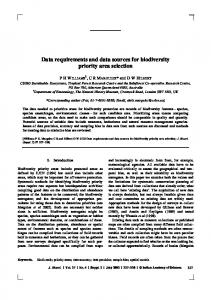
Data sets consist of areas and features. Areas are geographically defined units of land or water. They may be large or small, regular or irregular. Grid cells defined by latitude and longitude, catchments, tenure parcels, and fragments of native vegetation are some of the different kinds of areas used in conservation planning. Features are the properties of areas. Biodiversity features may be taxa or the characters they represent, or more heterogeneous entities such as assemblages or environmental classes, as discussed below. These features are actually biodiversity “surrogates” because they are used to stand for all of biodiversity. Ideally, data sets should convey a consistent sampling effort across the localities, biomes, and countries they cover because the identification of priority areas requires the systematic comparison of areas across all such regions. Consistency means that the preparation of data sets will probably involve some form of raw data analysis (Margules et al 1995). This analysis can include one or more of the following: classification of environmental variables; classification of biological records to derive, for example, species assemblages; and the estimation of wider spatial distribution patterns of species or assemblages with statistical or empirical models relating records of occurrence to environmental variables. Information about areas and biodiversity surrogates is most conveniently recorded and stored in an areas × features matrix. Features themselves can have different states. Figure 1 depicts three areas × features matrices. The first contains features of the ‘presence only’ kind in which species, for example, have been recorded as present in some areas but there is no indication of abundance or extent, and the lack of a recorded presence within other areas does not necessarily imply absence. Rather, it means that it is not known whether the feature occurs J. Biosci. | Vol. 27 | No. 4 | Suppl. 2 | July 2002

there or not. The second matrix contains ‘presence/ absence’ features. In this case the absences are real (within the limits of sampling intensity), meaning that the features were looked for and recorded as present where they were found and recorded as absent where they were not found. The third matrix contains estimates of abundance or extent, as well as absences. The methods for identifying priority areas can be applied to data sets with all three kinds of features with, successively, more confidence in the results. Some real-world applications of those methods have used matrices that were composites of each of these three types of data (e.g. RACAC 1996; Pressey 1998; Ferrier et al 2000). Unfortunately, almost all records of taxa are of the presence only kind. Most field records have been collected opportunistically, and the species collected are often the ones of interest to the collector. Many collections of field records map road networks (Margules and Austin 1994). It is often not possible to define the distribution patterns of species because there are few, if any, records of where they were looked for but not found. More systematic methods for the collection of new data are now available (Gillison and Brewer 1985; Austin and Heyligers 1989, 1991; Margules and Austin 1994; Wessels et al 1998), but still not widely utilized, perhaps because they are more extensive, but possibly because most data collections are still made for purposes other than identifying biodiversity priority areas. In the meantime, the best use has to be made of existing data, even if field records are geographically biased and incomplete. There are techniques available to estimate spatial distribution patterns from presence only data (Nix 1986; Margules et al 1995) and there are techniques for estimating underlying character difference among taxa (Vane-Wright et al 1991; Faith 1992a,b, 1994; Forey et al 1994; Humphries et al 1995). Both add value to existing data sets. 3.1

Biodiversity surrogates

Surrogates are needed because it is impossible to measure all of biodiversity. The task of discovering, naming, and then determining the systematic affinities of all species is daunting. Scientific names have been given to approximately 1⋅4 million species of plants, animals, and microorganisms (Wilson and Peters 1988; Ehrlich and Wilson 1991) but this is only a fraction of all species. Estimates of arthropod diversity in tropical forests alone range from about 7–80 million (Erwin 1982, 1983; Stork 1988; Hammond 1992), and other invertebrate phyla are even more poorly known. Estimates have been made that if the collection and description of new species were to continue at the current rate, using traditional methods, it would take several thousand years to catalogue the world’s biodiversity (e.g. Disney 1986; Soulé 1990), and

Representing biodiversity in fact the rate is slowing down because funding for taxonomy has declined (e.g. Stork and Gaston 1990; Whitehead 1990). Urgency has led to the development of methods for rapid biodiversity assessment. The idea is that semiprofessionals, variously referred to as apprentice curators (e.g. Sandlund 1991) or biodiversity technicians (Oliver and Beattie 1993), receive only basic training in field biology and systematics. They make field collections,

313

which they then sort, into broad taxonomic groups and morpho-species or recognisable taxonomic units (Oliver and Beattie 1993). In this way rapid estimates of morphospecies richness at particular sites or over particular areas can be made. The best developed program is in Costa Rica where an early goal was to obtain an inventory of Costa Rica’s biodiversity by the year 2000 (Janzen 1991). The energy and commitment of those involved in the Costa Rican

(A)

(B)

(C)

Figure 1. Three kinds of areas × features matrices showing (A) presence only data, (B) presence/absence data, and (C) abundance data. J. Biosci. | Vol. 27 | No. 4 | Suppl. 2 | July 2002

314


enterprise (see Gámez 1991; Sandlund 1991; Hovore 1991; Janzen 1991; Wille 1993 for comprehensive accounts) may have approached this goal, and it may eventually prove to be a model for other countries. Oliver and Beattie (1993) offer support with their finding that, with only basic training, biodiversity technicians were able to estimate to within 13%, the actual number of spider species, to within 6%, the actual number of ants, to within 38% the actual number of polychaetes, and to within 1% the actual number of mosses, in samples from Australia. But even if Costa Rica had reached its goal by the year 2000, or does so in the next few years, and even if biodiversity technicians can be enlisted and trained at a fast rate, the likelihood that even approximately full inventories will be available for most parts of the world in the short term, say 20 to 50 years, seems remote because such a colossal effort and vast resources would be required (e.g. Disney 1986). Even when inventories do become available they are, invariably, catalogues or lists of species for selected sites or, far less helpful, merely estimates of numbers of taxa from particular locations (if there is a lack of identity across samples from different areas they cannot be compared validly). The wider spatial distribution patterns of identified taxa will still have to be estimated (i.e. those raw data would still have to be analysed using spatial modelling techniques) before they could form an adequate data set for identifying biodiversity priority areas. In the short to medium term only groups of taxa representing a very small proportion of total biodiversity will be available for the identification of priority areas across extensive regions. Since complete inventories are not a practical option, yet land use change is proceeding apace, some measurable biodiversity surrogates are required. Realistically, there are three kinds available: sub-sets of taxa or higher taxa, assemblages, and environmental variables or classes. It is not possible at this stage to nominate one as better than the others because there are valid arguments, summarized below, for and against each of them. In reality some combination of these surrogates will have to be used in most cases to identify biodiversity priority areas because the data available will normally come from a variety of sources (see e.g. Nix et al 2000). 3.1a Sub-sets of taxa: Although there is disagreement among biologists about the definition of species, most people recognise the term and think they understand it. Species are the usual units with which diversity has been measured (Vane-Wright 1992). Higher taxa (e.g. genera, families) might also be used if a relationship between the distribution patterns of higher taxa and the distribution patterns of species can be demonstrated. For the same breadth of taxonomic coverage, it would be cheaper and J. Biosci. | Vol. 27 | No. 4 | Suppl. 2 | July 2002

easier to identify samples at higher taxon levels (Williams and Gaston 1994). In the short to medium term there may be little choice about sub-sets of taxa, because it depends on available data and available experts. However, if there is the opportunity to choose, then consideration should be given both to focal taxa (sensu Ryti 1992 – those we have good information about and are taxonomically tractable such as birds and vascular plants), and target taxa (sensu Kremen 1992 – those taxa that can be demonstrated to be better than average indicators of a wider range of biodiversity). Most taxa remain undescribed and even of the taxa that are known, only a small sub-set is sufficiently well studied, both in terms of taxonomic status and geographic distribution, to be used to identify priority areas. Unfortunately, there is no compelling evidence that sub-sets of taxa can represent biological diversity as a whole, even if the practicalities of conservation planning often require their use. Vane-Wright (1978) pointed out that, despite the coevolution theory for butterflies and plants, raw measures of plant diversity (family or species richness) were poor predictors of butterfly diversity on a global scale. Majer (1983) showed that variation in plant diversity accounted for only 24% of the variation in ant diversity in part of Western Australia. Yen (1987) found no correlation between the number of vertebrate species and the number of beetle species, and further, that neither beetle nor vertebrate communities corresponded to plant communities in south-eastern Australia. Prendergast et al (1993), Prendergast and Eversham (1997), and Williams and Gaston (1998) showed only partial correspondence between areas rich in butterflies, dragonflies, and breeding birds in the UK. Van Jaarsveld et al (1998) found little correspondence in the sets of areas chosen to represent various taxonomic groups in the Transvaal of South Africa. Williams and Gaston (1994) noted poor correlations among groups within continents, and Gaston et al (1995) showed similar weak relationships at the global scale. It therefore seems unlikely that priority areas identified using one or a few taxonomic groups as surrogates will adequately represent biodiversity as a whole, even though such analyses are valuable for action plans centred on particular groups such as birds. It is important to note, however, that this issue is far from resolved. For example, Howard et al (1998) showed that areas selected for one group of species in Uganda were often good at representing species in other groups. The studies on this aspect of biodiversity surrogacy have varied widely in geographic scale, the biogeographic histories of their study regions, and the methods used to measure the associations between the distributions of groups of taxa. Further, work on all three factors is necessary before the true worth of using sub-sets of taxa in conservation planning can be fully tested.

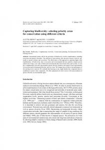
Representing biodiversity 3.1b Assemblages: The term assemblages is used here generically to cover a range of poorly-defined classifications such as community, association, habitat type, etc. They are generalized biological entities more heterogeneous than taxa (i.e. they are not monophyletic). Taxa are distributed patchily within them and may only be present at particular times. Assemblages can be subjectively derived using a small number of dominant or prominent species or they can be derived from field data with numerical pattern analysis techniques. Figure 2 is one classification that might result from a numerical pattern analysis of the data set illustrated in figure 1. Four classes have been recognised based on the biodiversity features they have in common. Areas O and P have two features in common not shared by any other areas. Areas L, M, and N have one feature in common not shared by any other areas. Areas F, G, H, I, J, and K all have at least three features in common and, although two of those are shared by some other areas, they also share a number of other features in various combinations. Areas A, B, C, D, and E share one feature also shared by most other areas, but what they really have in common is the absence of most other features. In real data sets, areas and features can number in the order of thousands, and classification and ordination can help simplify such complex multi-variate data, and help reveal underlying patterns. Basic texts on these kinds of analyses with a biological emphasis include Clifford and Stephenson (1975), Williams (1976), and Gauch (1982). Unlike taxa (which have properties of both classes and individuals: Nelson 1985), assemblages are simply classi-

315

fications of co-occurring species. Assemblages, however, have an additional property of representing various alternative combinations of species and the interactions between them, and therefore more ecological complexity than individual taxa. Larger organisms such as vascular plants and vertebrates, those most often used to delineate assemblages, interact with, and therefore encompass spatially, smaller organisms such as nematodes, arthropods, fungi, protozoa, and bacteria, taxonomic groups which are usually ignored in conservation planning but are much more speciose than groups representing larger organisms (McKenzie et al 1989). On the other hand, protecting a single area as a representation of an assemblage is likely to miss some species (Pressey 1992) and some ecological complexity, because it may be impossible to judge whether or not a given part of an assemblage is an adequate representation of the whole. 3.1c Environments: Environment is also a generic term covering land classifications based primarily on physical and climatic variables, numerical or intuitive, which may or may not incorporate some biotic variables such as vegetation. Land systems (Christian and Stewart 1968) are examples of intuitive classifications, while environmental domains (e.g. Mackey et al 1989; Faith et al 2001b) are examples of numerical classifications. Similar classifications can be used in aquatic environments (e.g. Ward et al 1998). Environmental variables may also be used unclassified, to represent environmental heterogeneity and, therefore, as biodiversity surrogates (Faith and Walker 1996a). Different kinds of environments are

Figure 2. Four groups of areas that might be recognized using numerical clustering based on shared features. J. Biosci. | Vol. 27 | No. 4 | Suppl. 2 | July 2002

316


assumed to support different sets of species (with some overlap) and have been used at broad scales as biodiversity surrogates (e.g. Mackey et al 1989; Richards et al 1990; Belbin 1993; Pressey et al 1996). There is theoretical support for the use of environments as biodiversity surrogates, which can be summarized as follows (Margules and Austin 1994): each species has a unique distribution within environmental space determined by its genetic make-up and physiological requirements. This distribution is, in turn, constrained by ecological interactions with other species. This is the concept of the niche (Hutchinson 1958). Plant ecologists use the term ‘individualistic continuum’ for essentially the same concept (Austin 1985). Species respond individualistically in, say, abundance or frequency, to resource gradients, and that response is constrained by interactions with other species. The implications are three-fold. First, each species occupies a unique niche not necessarily predictable from that of other species (i.e. there is little overlap in environmental space between many species, although much overlap between some). Second, and related to the previous point, species distribution patterns are most accurately measured in multi-dimensional environmental space and only then translated to geographic space. Third, the resultant spatial pattern shows high or dense populations in scattered locations representing the most favourable habitat (or mix of environmental variables) and lower, more sparse populations in areas of less favourable habitat. Thus, the geographic distribution patterns of species can be linked to variation in the environment. Whittaker (1956, 1960), Perring (1958, 1959), and Austin et al (1984, 1990), among others, have provided empirical support. Nix (1982, 1986) has argued that, for many purposes, including estimating the spatial distribution patterns of species, complete niche specification is unnecessary and that in most cases, five regimes, namely solar radiation, temperature, moisture, mineral nutrients, and other components of the biota, are sufficient. A network of priority areas that represents the range of environmental combinations in a region is likely to encompass unknown species and known species with distribution patterns that are incompletely described. Furthermore, the data needed to delineate environments (e.g. climatic data, geology maps, etc.) are more generally available at a consistent level of detail across wide geographic areas, than are field records of species occurrences. On the other hand, as is the case with assemblages, protecting a single area as a representation of an environment is likely to miss some species because it is not clear what an adequate representation might be. Similarly, the relationships between environmental classes and the distribution and abundance patterns of taxa can be unclear and difficult to quantify, and some species J. Biosci. | Vol. 27 | No. 4 | Suppl. 2 | July 2002

may require a combination of environmental variables not recognised by a classification (Pressey 1992). Furthermore, environmental approaches must make bold assumptions about the uniformity of the distribution patterns of species in niche space and, perhaps with greater risk, must assume that species distributions are at equilibrium with governing environmental factors, thereby ignoring the potential role of metapopulation dynamics in the regional persistence of species. 3.1d Combinations of surrogates: Taking into account the limitations on current knowledge, the limited resources for acquiring new data, and the goal of adequately representing each surrogate, it seems likely that in practice some combination of these surrogates will be most widely applicable (see Nix et al 2000 and Faith et al 2001a for practical applications). In many localities some data on the distributions of taxa are available, but at an inconsistent level of detail and geographically biased. It may be that areas with endemic taxa, especially endemic vertebrates and plants, have been identified, because these areas are inherently interesting to naturalists. Usually, at least some environmental data are available at a consistent level of detail and it may be that assemblages have been mapped as, for example, vegetation or habitat types. One way to proceed in such cases would be to represent each environment or assemblage, overlay available distribution maps of taxa and/or areas of endemicity to see which, if any, were still not represented, and add areas to complete the representation (Noss 1987; Nicholls and Margules 1993; Noss et al 1999). Alternatively, the geographic locations of selected taxa, such as rare or vulnerable species, or areas of endemicity, could be used as seed points around which to build up a representation of each environment (e.g. Bull et al 1993). There are problems with both of these approaches, though, because of the geographical bias of most field records, and because strict reservation may not be the most appropriate protection for rare or vulnerable species. Management to alleviate threatening processes, perhaps without changing the tenure of the areas concerned, may be more appropriate for localized species of concern. Spatial modelling based on species localities can help alleviate the first problem, but it seems likely that some level of spatial bias will have to be accepted in most conservation planning exercises.

3.2

Collecting new data

It may be necessary or desirable to collect new biological data. If the resources are available for doing so, then the most effective use should be made of them, and new collecting activities, if any, should provide data that can

Representing biodiversity be analysed in a way that maximizes the information gained. In particular, new data should be collected in a way that facilitates accurate estimation of the spatial distribution patterns of species or other biodiversity surrogates. The collection and analysis of new data should be based on an explicit set of assumptions: a conceptual framework based on current ecological theory, which indicates environmental stratification to ensure that the entire range of combinations of environmental variables is sampled; field survey design principles based explicitly on the conceptual framework for locating field sample sites; a rationale for deciding which measurements should be made at field sample sites in addition to records of the target species; and appropriate analytical methods for estimating wider spatial distribution patterns from the point records that field sample sites represent. Austin and Heyligers (1989, 1991), Nicholls (1989, 1991) and Margules and Austin (1994) explain how the steps involved in implementing this protocol can be put into practice. The result would be a data base consisting of presence-absence records. Data of this kind are more reliable and amenable to spatial modelling than presence only data (Williams et al 2002). While some parts of suitable habitat may still be unoccupied at any given time, for example when the survey takes place, this sort of data set is a substantial improvement on presence-only data sets.

GAMs (e.g. Austin and Meyers 1996). Empirical models are for data of the presence only kind. That is, there are records of where a taxon occurs but it is not known whether a non-occurrence is a true absence or simply a result of the taxon not having been looked for there. Almost all museum and herbarium accessions, one of the most common and widely available sources of field records, are of this kind. Statistical models are appropriate for data of the presence/absence kind. That is, the absence of a species is the result of it having been looked for but not found. The other option is to classify the data into assemblages and map their boundaries. Classification can be done intuitively or with numerical methods, and mapping can be intuitive or it can utilize computer based empirical or statistical methods. Similarly, if the intention is to use environmental classes, classification can be intuitive or numerical, and mapping can be manual or computer based. Whether it is biological, environmental or a combination of both, the end result is a data set that contains maps (on paper or in electronic form) of the chosen biodiversity surrogates. This data set can then be used, with the methods summarized below, to identify biodiversity priority areas.

4. 3.3

Summary of data requirements

The features used in areas × features matrices for identifying priority areas are always surrogates for the whole of biodiversity. Biodiversity surrogates may be taxa (e.g. species), species assemblages, and environmental classes or variables, or they may be combinations of these. Compiling a data set for conservation planning is a process that includes both acquiring relevant data and, in most cases, analysing those data (classification, ordination, and/or mapping) so that they are in a form suitable for identifying biodiversity priority areas. Biological data in the form of records of the geographic locations of taxa may be available from previous collecting expeditions or surveys, or collected during new surveys. Environmental data may be extracted, for example, from meteorological records and topographic maps, and from existing thematic maps of geology and soils. For the analysis of data in the form of species records there are two general options. One is to estimate the geographic distribution patterns of taxa, either intuitively, or by relating actual records of locations to environmental variables using predictive empirical models such as BIOCLIM (Nix 1986; Busby 1986, 1991), or statistical models such as GLMs (e.g. Nicholls 1989, 1991) and

317

Identifying biodiversity priority areas

Biodiversity priority areas should, collectively, represent the biodiversity of the locality or region they are situated in; that is, they should encompass all of the biodiversity features (species, assemblages, environments) in the data set. Inevitably, areas and/or features such as species will be prioritized because not all are subjected to the same degree of threat. A remote area in rugged terrain, for example, may not require the same allocation of scarce management resources as a remnant of natural habitat in an agricultural district. Effective protection need not necessarily require formal reservation because in some cases it may be possible to treat areas as protected if a current land use is compatible and likely to continue. In other cases, formal protection measures and appropriate management can sometimes be put in place without the need for change in ownership (Moore 1987; Edwards and Sharp 1990; Farrier 1995; Keith 1995; Bean and Wilcove 1997; Knight 1999). Methods for identifying priority areas are therefore only one aspect of overall biological conservation planning and management (Margules and Pressey 2000; Gaston et al 2002). In the past, parks and reserves, areas currently protecting components of biodiversity had been set aside primarily for reasons other than the representation of biological diversity. The earliest National Parks, e.g. J. Biosci. | Vol. 27 | No. 4 | Suppl. 2 | July 2002

318


Yellowstone in the USA and Royal, near Sydney, Australia, were chosen primarily for their outstanding scenic and recreational values. Many areas throughout the world continue to be set aside for similar reasons, or, for example, because they protect particular rare species or wilderness areas. A widespread tendency, however, appears to be that areas are reserved because they have little potential for commercial exploitation or human habitation (e.g. Runte 1979; Kirkpatrick 1987; Henderson 1992; Pressey 1994; Rebelo 1997; Barnard et al 1998; Pressey et al 2000). Thus, in general, the establishment of reserves has been ad hoc in the sense of failing to address any strategic regional priorities for the protection of biodiversity. This is despite the goal of representing natural variety in reserves being explicit since the 1930s in the United States (Noss and Cooperrider 1994) and since the 1940s in New South Wales (Strom 1990). Ad hoc reservation has proceeded despite the goal of representativeness, not because of its absence, and has had three unfortunate results. First, the biodiversity (taxa, assemblages, environments) most in need of strict reservation in regions has often not been protected (Pressey and Tully 1994). Consequently and second, limited conservation resources have been used inefficiently in that current protected areas contain relatively few biodiversity surrogates or those that are not in most urgent need of protection (Awimbo et al 1996). Third, therefore, there is now a very uneven representation of biodiversity in existing reserves (Leader-Williams et al 1990; Pressey et al 1993, 2000). Scoring and ranking procedures were developed in an attempt to make priority setting more systematic and explicit. In these procedures, multiple criteria, e.g. diversity, rarity, naturalness, and size, among others, are given scores. These scores are then combined for each candidate area. The areas are then ranked and highest priority is given to the areas with the highest scores. There have been many critical reviews of these procedures and the criteria used (e.g. Margules and Usher 1981; Margules 1986; Smith and Theberge 1986, 1987; Usher 1986) but it was not until Pressey and Nicholls (1989) examined their efficiency that a fundamental problem with their ability to achieve the goal of full representation of natural features was uncovered. In summary, Pressey and Nicholls (1989) found that selecting areas downwards from the one ranked highest, based on a variety of different scores, required at least a fifth, but in most cases more than half, of all areas if full representation was to be achieved. Application of scoring and ranking procedures does not improve efficiency greatly over ad hoc representation. The selection methods summarized below are designed to help remedy current uneven representation and promote efficiency. They are based on three groups of interrelated principles; persistence and vulnerability, complemenJ. Biosci. | Vol. 27 | No. 4 | Suppl. 2 | July 2002

tarity and efficiency, and irreplaceability and flexibility. Efficiency is important because the amount of land or water realistically available for biodiversity protection is limited. The real prospect exists that upper limits of land available for protection will be reached in many regions well before their biodiversity is adequately represented (and, therefore, its persistence in the landscape reasonably assured). An actual example comes from the forests of south-eastern New South Wales where politically imposed ceilings on the reserve system, both in terms of hectares and timber volume unavailable to industry (RACAC 1996), have now been reached but the reserve system still does not contain some of the most depleted and threatened vegetation types (Keith and Bedward 1999). Explicitness in selection procedures is also important. One reason is that, for the results to be verifiable independently, they must be repeatable. Another is that priority area networks so identified can be justified and understood more easily, and thus defended more readily (Margules et al 1994), so helping to build a broader consensus.

4.1 Persistence and vulnerability Some ecosystems and the biota they contain are more vulnerable to threatening processes than others. Fertile soils and good rainfall are conducive to agricultural production, for example. Similarly, some species cope well with impacts such as habitat fragmentation and grazing, being favoured by the changed conditions, while others suffer a reduction in abundance, a contraction of range and even, in some cases, local or global extinction. In many situations it may be possible to predict which kinds of habitats or ecosystems are most likely to be exploited (Benson and Howell 1990; Pressey et al 1996a; White et al 1997; Mittermeier et al 1998; Paal 1998) and in some cases it may be possible to predict which species will cope well with exploitation of their habitat and which species will not (e.g. Bink 1992; Bodmer et al 1997; Kirchhofer 1997; McKinney 1997; Burgman et al 1999; Davies et al 2000). This kind of information on vulnerability or threat can be used to help set the goals of a priority area selection procedures (Gaston et al 2002). Because resources for conservation planning are limited, not all biomes, parts of countries, whole countries, or regions can be dealt with equally or at the same time. In identifying priority area networks, preference should be given to places that are both vulnerable to a threatening process such as land clearing for agriculture and also make an important contribution to the conservation goal. Alternatively, the goal might be to represent species that are vulnerable to threatening processes, rather than all the species in a

Representing biodiversity region, in which case the data set being used would contain only those species. Persistence relates more to the long-term viability of species in areas established for the protection of biodiversity (Gaston et al 2002). Persistence depends on many factors, including the representation goal set for biodiversity surrogates, the size, shape and connectedness of reserves, the extent to which reserves replicate features as a form of insurance against local extinction, the extent to which species protected now will be able to adjust their ranges in response to climate change, the viability of populations in terms of both size and demographic characteristics and the resources available for ongoing management of reserves so that natural processes continue and the effects of adverse human impacts are minimized. Persistence can also be taken into account by assigning probabilities of persistence to the features occurring in areas according to the suitabilities of those areas for alternative land uses, setting the conservation goal to be a given probability that all surrogates persist (e.g. 0⋅99), and then testing different regional planning scenarios by estimating the extent to which the goal will be compromized by the removal of areas (Faith et al 2001c). 4.2

Complementarity and efficiency

The selection of priority areas has to proceed from the goal of representing all biodiversity surrogates, and must

319

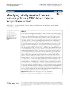
not be side-tracked by other equally legitimate but different goals, such as the preservation of scenic landscapes or wilderness (Sarkar 1999), although areas that contribute importantly to divergent goals may sometimes coincide. Thus, any new areas added to an existing priority area network should contribute new features unless all of them are already represented. This common sense observation reflects the principle of complementarity (Vane-Wright et al 1991). Priority areas should complement one another in terms of the features they contain; the characters, taxa, assemblages, environments, etc. It follows that an area contributing most to completing a full complement will not necessarily be the richest area (Knopf and Samson 1994), and this, in fact, is often the case. Indeed, under some circumstance, sets of rich areas may contain no more species in total than would be expected from choosing the same number of areas at random (Williams et al 1999). This is why ranking procedures, such as selecting a sub-set of richest areas, are often so inefficient. They fail to take account of spatial heterogeneity and the turnover of features from area to area (and see Howard et al 1998). Complementarity is a property of areas within the areas × features matrix. It is a measure of the extent to which an area, or set of areas, contributes unrepresented features to an existing set of areas (Faith 1994). Figure 3 is another representation of the data matrix shown in figures 1 and 2. There is a total of 15 species in the matrix in figure 3. Area G has two unique species and

Figure 3. The species represented at each step of an application of complementarity. Area G selected at the first step represents species 1–7. Area O selected at the second step adds species 9, 10, 14, and 15. Area J selected at the third step adds species 8, 11, and 12. At the fourth step, any one of areas L, M, or N would add the remaining species, 13. J. Biosci. | Vol. 27 | No. 4 | Suppl. 2 | July 2002

320


five others shared by one or more other areas. Imagine area G has been identified as a biodiversity priority area because of its two unique species. Seven of the 15 species are represented in area G. The remainder is the residual complement; species 8 to 15. Area O contains four species from that unrepresented complement, more than any other area. If area O were added to area G as a second biodiversity priority area, 11 species would be represented, leaving a residual complement of just four. Area J contains three of those four. If area J were added to the network it would leave a residual complement of just one species, which could be represented by any one of areas L, M, or N. This illustrates an iterative heuristic procedure, which measures the unrepresented complement in each area at each step and adds the area with the largest unrepresented complement until the total complement is represented (e.g. Kirkpatrick 1983). A similar heuristic algorithm (Margules et al 1988; Nicholls and Margules 1993) selects areas with the rarest features first and then adds areas with the rarest remaining unrepresented features until all are represented. Thus, area G would still be chosen first but J would be chosen second. They both have seven species and both have two unique species, but G additionally contains one species (species 5) present in only two areas, whereas the next rarest species in area J (after the unique species) is present in four areas altogether (species 8). The next choice would be between areas O and P which both have the rarest remaining species (species 14 and 15), and O would be chosen because it contributes those two next rarest species plus two others not yet represented (species 9 and 10). Once again, the last unrepresented species (species 13) could be represented by any one of areas L, M, or N. In this example the list of areas chosen is the same, but the order is different. Using other data sets, the lists might differ between the two algorithms. These examples assume that the conservation goal is to represent at least one occurrence of each of the species in figure 3. If the data matrix were composed of the extent of each of fifteen vegetation types in each of the sixteen areas (similar to the matrix in figure 1c) and the conservation goal were expressed as hectares of vegetation types (e.g. at least 150 ha of each), the order of selection of each of the two algorithms described above, and the lists of selected areas, might be very different. In this case, selecting an area might not fully achieve the goal for the vegetation types it contains and other areas with some of the same vegetation types might also need to be selected. In other words, the complementarity of the areas would be different. The operations of all systematic methods for conservation planning depend critically on how the conservation goal is defined. J. Biosci. | Vol. 27 | No. 4 | Suppl. 2 | July 2002

Alternatives to iterative heuristics, such as linear programming (Cocks and Baird 1989; Underhill 1994; Csuti et al 1997; Ando et al 1998; and see Pressey et al 1996b, for a critique) also employ complementarity (Vane-Wright 1996). Complementarity is important because it leads to an efficient representation of biodiversity features and, therefore, an efficient use of limited conservation resources such as land (or water) and funds. Algorithms which incorporate complementarity procedures are much more efficient than ad hoc approaches (Pressey and Tully 1994) and scoring and ranking approaches (Pressey and Nicholls 1989).

4.3

Irreplaceability and flexibility

Figure 3 also illustrates the principles of flexibility and irreplaceability. Areas G and J are irreplaceable because they contain unique species (species 6 and 7, and 11 and 12, respectively). Areas L, M, and N all contribute the same species to the full complement so they can be substituted for one another. They are replaceable. Area O is also replaceable, though less so than L, M, and N because two of its species occur in only one other area. Area O contributes four species to the full complement. Those same four could not be contributed by any other single area, but area P plus either H or I could be substituted for O. These have been described as different levels of irreplaceability (e.g. Pressey et al 1993, 1994; Ferrier et al 2000). Areas G and J are globally irreplaceable. Area O is goal irreplaceable (Rebelo 1994) because the goal is to find the fewest areas that represent all species. It would cost an extra area to replace O. Areas L, N, and M are all replaceable (in this case, each with either of the other two). When data matrices contain the extent or abundance of each feature (e.g. figure 1c) and the conservation goal is also expressed as an extent or abundance of each feature, areas can be irreplaceable for three reasons: first, because the area contains one or more unique features; second, because the area contains one or more non-unique features and the conservation goal is equal to their total remaining extent; or third, because the area contains occurrences of one or more non-unique features that are sufficiently large that the goal cannot be achieved without conserving that area. Like complementarity, the irreplaceability of areas depends critically on how the conservation goal is defined. The existence of replaceable areas, which may be rare in some cases (Rebelo 1994) but seems to be common in many data sets (e.g. Pressey et al 1994; Rebelo and Siegfried 1992) facilitates negotiation over the location of new priority areas relative to competing land uses (Pressey 1998, Ferrier et al 2000). All replaceable areas

Representing biodiversity are negotiable, though some have associated costs, such as the extra area needed if area O in figure 3 were not available. Globally irreplaceable areas are not negotiable because without them it would be impossible to achieve the goal of representing all features. They should form the core around which the rest of a priority area network is built. Flexibility is a property of the network of areas. It arises because many of the areas needed to fulfil the representation goal can be replaced by one or more others. Flexibility refers to the different spatial arrangements of areas available to achieve the goal.

4.4

Implementation

Fully complementary priority area networks can be identified using heuristic iterative or set-wise procedures relatively simply, once goals have been agreed upon and data are available, but implementation in the real world is more problematic (Margules and Pressey 2000). Some areas may be unsuitable because, for example, they are degraded, or simply unavailable for compelling social, economic, or political reasons. Flexibility in spatial configuration can help find practical solutions but even when pragmatic compromises have been made, not all nominal priority areas will have equal status. It is likely that priorities within any identified network of priority areas will have to be set. The impacts of threatening processes will affect both the timing of protection and the type of protection measure applied Areas that are more vulnerable to threatening processes would have a higher priority, but it may be necessary to examine them closely before coming to any final decision. For example, consider a habitat remnant in cropland and a more remote site in rugged terrain. They occupy different environments and contribute different features to the full complement, but the habitat remnant is more vulnerable simply because of its location. If it were determined that the habitat remnant was seriously threatened, or that populations of taxa there had low probabilities of persistence unaided, then it might be accorded priority and scarce management resources might be allocated in an attempt to protect it. On the other hand, if the area occupied by the remnant was not irreplaceable, alternatives could be sought. Even if the remnant were irreplaceable, it is conceivable that a greater contribution to the overall conservation goal might be obtained by abandoning it and diverting scarce management resources elsewhere, particularly if it were assessed to have low viability even if given intensive management. However, it is better to have known in the first place which biodiversity surrogates the remnant contributed and whether it was irreplaceable, so that the trade-off between allocating management resources and compromising the goal

321

of representation could be made on the basis of all possible information.

5.

Summary

The problem addressed above is how to measure the contribution of different areas in a region to a conservation goal, which is some agreed level of representation of the biological diversity of that region. The aim is to ensure, as far as possible, the persistence of biodiversity (its components, hierarchical levels, and ecological processes) in the landscape. Areas with a high contribution, because of high complementarity and/or irreplaceability (and note that some areas can have high values for both), are called biodiversity priority areas. Because total biodiversity as it is interpreted here is not directly measurable, it will only ever be possible to represent surrogate features: sub-sets of taxa, assemblages, and/or environments and environmental variables. Two classes of methods are required (Margules et al 1995). The first includes methods for deriving suitable data sets; the second, methods for using those data to identify priority areas. Raw data in the form of climatic data or field records of the locations of taxa, for example, can be treated in various ways to improve their quality and utility, such as modelling wider spatial distribution patterns (Williams et al 2002) or estimating character diversity from phylogenetic patterns (Williams et al 2002). If new data can be collected then this should be done in a more systematic, cost-effective way than it often has been in the past, enabling more accurate statistical models of spatial distribution patterns to be derived (Austin and Heyligers 1989; Margules and Austin 1994). The methods described here for identifying priority areas are efficient and explicit heuristic algorithms. They employ the principles of complementarity, flexibility, and irreplaceability. Their goal is to represent all of the biodiversity features in the available data set in as few areas as possible (or as many viable features as possible for a given number of areas, or total area), which should be the starting point for biodiversity conservation planning. Preferred priority areas can then be determined via an exploration of flexibility and possible alternative configurations, and an assessment of the costs associated with controlled departures from the most efficient representation, to facilitate negotiation with competing land uses. Two major case studies of real-world applications have now been completed, one in the forests of north-eastern New South Wales (Pressey 1998) and the other a country wide conservation plan for Papua New Guinea (Nix et al 2000; Faith et al 2001a). Another major exercise using the methods outlined here is underway in the Cape Floristic Region of South Africa (Cowling et al J. Biosci. | Vol. 27 | No. 4 | Suppl. 2 | July 2002


322

1999), one of the most widely recognised global hotspots for biodiversity conservation (Myers et al 2000). Biodiversity priority areas are necessary but not sufficient for the long-term maintenance of biological diversity. The methods summarized above are some of the tools needed by conservation biologists to help them identify priority areas. Other tools, such as management prescriptions to minimize the risk of extinction of local populations, can then be focused more sharply on the places and populations in greatest need. References Abate T 1992 Environmental rapid-assessment programs have appeal and critics; BioScience 42 486–489 Ackery P R, Smith C R and Vane-Wright R I (eds) 1995 Carcasson’s African butterflies: an annotated catalogue of the Papilionoidea and Hesperioidea of the Afrotropical region (Melbourne: CSIRO) Ackery P R and Vane-Wright R I 1984 Milkweed butterflies (Cornell: Cornell University Press) Adam P 1992 The end of conservation on the cheap; Natl. Parks J. 36 19–22 Aiken S R 1994 Peninsular Malaysia’s protected areas’ coverage 1903–92: creation, rescission, excision, and intrusion; Environ. Conserv. 21 49–56 Ando A, Camm J, Polasky S and Solow A 1998 Species distributions, land values, and efficient conservation; Science 279 2126–2128 Austin M P 1985 Continuum concept, ordination methods and niche theory; Annu. Rev. Ecol. Syst. 16 39–61 Austin M P and Heyligers P C 1989 Vegetation survey design for conservation: gradsect sampling of forests in northeastern New South Wales; Biol. Conserv. 50 13–32 Austin M P and Heyligers P C 1991 New approaches to vegetation survey design: gradsect sampling; in Nature conservation: cost effective biological surveys and data analysis (eds) C R Margules and M P Austin (Melbourne: CSIRO) pp 31–36 Austin M P, Cunningham R B and Fleming P M 1984 New approaches to direct gradient analysis using environmental scalars and statistical curve-fitting procedures; Vegetatio 55 11–27 Austin M P and Meyers J A 1996 Current approaches to modelling the environmental niche of eucalypts: implications for management of forestry; For. Ecol. Manag. 85 95–106 Austin M P, Nicholls A O and Margules C R 1990 Measurement of the realised qualitative niche: environmental niches of five Eucalyptus species; Ecol. Monogr. 60 161–177 Awimbo J A, Norton D A and Overmars F B 1996 An evaluation of representativeness for nature conservation, Hokitika ecological district, New Zealand; Biol. Conserv. 75 177–186 Barnard P, Brown C J, Jarvis A M and Robertson A 1998 Extending the Namibian protected area network to safeguard hotspots of endemism and diversity; Biodiver. Conserv. 7 531–547 Bean M J and Wilcove D S 1997 The private-land problem; Conserv. Biol. 11 1–2 Beardsley K and Stoms D 1993 Compiling a map of areas managed for biodiversity in California; Nat. Areas J. 13 177– 190

J. Biosci. | Vol. 27 | No. 4 | Suppl. 2 | July 2002

Belbin L 1993 Environmental representativeness: regional partitioning and reserve selection; Biol. Conserv. 66 223–230 Benson D H and Howell J 1990 Sydney’s vegetation 1788– 1988: utilization, degradation and rehabilitation; Proc. Ecol. Soc. Aust. 16 115–127 Bink F A 1992 The butterflies of the future, their strategy; in Future of butterflies in Europe: strategies for survival (eds) T Pavlick-van Beek, A H Ovaa and J G van der Made (The Netherlands: Department of Nature Conservation, Agricultural University of Wageningen) pp 134–138 Bodmer R E, Eisenberg J F and Redford K H 1997 Hunting and the likelihood of extinction of Amazonian mammals; Conserv. Biol. 11 460–466 Bull A L, Thackway R and Cresswell I D 1993 Assessing conservation of the major Murray-Darling ecosystems [Canberra: Environmental Resources Information Network (ERIN), Australian Nature Conservation Agency] Burgman M A, Keith D A, Rohlf F J and Todd C R 1999 Probabilistic classification rules for setting conservation priorities; Biol. Conserv. 89 227–231 Busby J R 1986 A biogeoclimatic analysis of Nothofagus cunninghamii (Hook.) Oerst. in southeastern Australia; Aust. J. Ecol. 11 1–7 Busby J R 1991 BIOCLIM – a bioclimatic analysis and prediction system; in Nature conservation: cost effective biological surveys and data analysis (eds) C R Margules and M P Austin (Melbourne: CSIRO) pp 64–68 Caughley G 1994 Directions in conservation biology; J. Anim. Ecol. 63 215–244 Christian C S and Stewart G A 1968 Methodology of integrated surveys; in Proceedings of the Toulouse conference on aerial surveys and integrated studies (Paris: UNESCO) pp 233– 280 Clifford H T and Stephenson W 1975 An introduction to numerical classification (New York: Academic Press) Cocks K D and Baird I A 1989 Using mathematical programming to address the multiple reserve selection problem: an example from the Eyre Peninsula, South Australia; Biol. Conserv. 49 113–130 Commonwealth of Australia 1995 National Forest Conservation Reserves: Commonwealth Proposed Criteria (Canberra: Australian Government Publishing Service) Cowling R M, Pressey R L, Lombard A T, Heijnis C E, Richardson D M and Cole N 1999 Framework for a conservation plan for the Cape Floristic Region (Cape Town: University of Cape Town, Institute for Plant Conservation Report 9902) Csuti B, Polasky S, Williams P H, Pressey R L, Camm J D, Kershaw M, Kiester A R, Downs B, Hamilton R, Huso M and Sahr K 1997 A comparison of reserve selection algorithms using data on terrestrial vertebrates in Oregon; Biol. Conserv. 80 83–97 Davies K F, Margules C R and Lawrence J F 2000 Which traits of species predict population declines in experimental forest fragments?; Ecology 81 1450–1461 Disney R H L 1986 Inventory surveys of insect faunas: discussion of a particular attempt; Antenna (London) 10 112–116 Edwards V M and Sharp B M H 1990 Institutional arrangements for conservation on private land in New Zealand; J. Environ. Manag. 31 313–326 Ehrlich P R and Wilson E O 1991 Biodiversity studies: science and policy; Science 253 758–762 Eldredge N and Salthe S N 1984 Hierarchy and evolution; in Oxford surveys in evolutionary biology (eds) R Dawkins and

Representing biodiversity M Ridley (Oxford: Oxford University Press) vol. 1, pp 184– 208 Erwin T L 1982 Tropical forests: their richness in Coleoptera and other arthropod species; Coleopterists’ Bull. 36 74– 75 Erwin T L 1983 Tropical forest canopies: the last biotic frontier; Bull. Entomol. Soc. Am. 30 14–19 Faith D P 1992a Conservation evaluation and phylogenetic diversity; Biol. Conserv. 61 1–10 Faith D P 1992b Systematics and conservation: on predicting the feature diversity of subsets of taxa; Cladistics 8 361– 373 Faith D P 1994 Phylogenetic pattern and the quantification of organismal biodiversity; Philos. Trans. R. Soc. London B345 45–58 Faith D P and Walker P A 1996a Environmental diversity: on the best-possible use of surrogate data for assessing the relative biodiversity of sets of areas; Biodiver. Conserv. 5 399– 415 Faith D P and Walker P A 1996b Integrating conservation and development: incorporating vulnerability into biodiversityassessment of areas; Biodiver. Conserv. 5 417–429 Faith D P, Margules C R and Walker P A 2001a A biodiversity conservation plan for Papua New Guinea based on biodiversity trade-offs analysis; Pacific Conserv. Biol. 6 304– 324 Faith D P, Margules C R, Walker P A, Stein J and Natera G 2001b Practical application of biodiversity surrogates and percentage targets for conservation in Papua New Guinea; Pacific Conserv. Biol. 6 289–303 Faith D P, Walker P A and Margules C R 2001c Some future prospects for systematic biodiversity planning in Papua New Guinea – and for biodiversity planning in general; Pacific Conserv. Biol. 6 325–334 Farrier D 1995 Policy instruments for conserving biodiversity on private land; in Conserving biodiversity: threats and solutions (eds) R A Bradstock, T D Auld, D A Keith, R T Kingsford, D Lunney and D P Sivertsen (Sydney: Surrey Beatty) pp 337–359 Ferrier S, Pressey R L and Barrett T W 2000 A new predictor of the irreplaceability of areas for achieving a conservation goal, its application to real-world planning, and a research agenda for further refinement; Biol. Conserv. 93 303–325 Ferrier S and Watson G 1997 An evaluation of the effectiveness of environmental surrogates and modelling techniques in predicting the distribution of biological diversity (Canberra: Environment Australia) Forey P L, Humphries C J and Vane-Wright R I (eds) 1994 Systematics and conservation evaluation (Oxford: Oxford University Press) Freitag S, Nicholls A O and van Jaarsveld A S 1996 Nature reserve selection in the Transvaal, South Africa: what data should we be using?; Biodiver. Conserv. 5 685–698 Gámez R 1991 Biodiversity conservation through facilitation of its sustainable use: Costa Rica’s National Biodiversity Institute; Trends Ecol. Evol. 6 377–378 Gaston K J, Pressey R L and Margules C R 2002 Persistence and vulnerability: retaining biodiversity in the landscape and in protected areas; J. Biosci. (Suppl. 2) 27 361–384 Gaston K J, Williams P H, Eggleton P J and Humphries C J 1995 Large scale patterns of biodiversity: spatial variation in family richness; Proc. R. Soc. London B260 149–154 Gauch H G 1982 Multivariate analysis in community ecology (Cambridge: Cambridge University Press)

323

Gillison A N and Brewer K R W 1985 The use of gradient directed transects in natural resource surveys; J. Environ. Manag. 20 103–127 Hammond P M 1992 Species inventory; in Global biodiversity: status of the Earth’s living resources (ed.) B Groombridge (London: Chapman and Hall) pp 17–39 Henderson N 1992 Wilderness and the nature conservation ideal: Britain, Canada and the United States contrasted; Ambio 21 394–399 Hovore F T 1991 INBio: by biologists, for biologists; Am. Entomol. (Fall 1991) 157–158 Howard P C, Viskanic P, Davenport T R B, Kigenyi F W, Baltzer M, Dickinson C J, Lwanga J S, Matthews R A and Balmford A 1998 Complementarity and the use of indicator groups for reserve selection in Uganda; Nature (London) 394 472–475 Hughes J B, Daily G C and Ehrlich P R 1997 Population diversity: its extent and extinction; Science 278 689–692 Humphries C J, Williams P H and Vane-Wright R I 1995 Measuring biodiversity value for conservation; Annu. Rev. Syst. Ecol. 26 93–111 Hutchinson G E 1958 Concluding remarks; Cold Spring Harbor Symp. Quant. Biol. 22 415–427 JANIS (Joint ANZECC/MCFFA National Forest Policy Statement Implementation Sub-committee) 1997 Nationally agreed criteria for the establishment of a comprehensive, adequate and representative reserve system for forests in Australia (Canberra: Commonwealth of Australia) Janzen D H 1991 How to save tropical biodiversity: the National Biodiversity Institute of Costa Rica; Am. Entomol. (Fall 1991) 159–171 Keith D A 1995 Involving ecologists and local communities in survey, planning and action for conservation in a rural landscape: an example from the Bega Valley, New South Wales; in Nature conservation 4 – the role of networks (eds) D A Saunders, J L Craig and E M Mattiske (Sydney: Surrey Beatty) pp 385–400 Keith D A and Bedward M 1999 Native vegetation of the south east forests region, Eden, New South Wales; Cunninghamia 6 1–218 Kirchhofer A 1997 The assessment of fish vulnerability in Switzerland based on distribution data; Biol. Conserv. 80 1–8 Kirkpatrick J B 1983 An iterative method for establishing priorities for the selection of nature reserves: an example from Tasmania; Biol. Conserv. 25 127–134 Kirkpatrick J B 1987 Forest reservation in Tasmania; Search 18 138–142 Knight R L 1999 Private lands: the neglected geography; Conserv. Biol. 13 223–224 Knopf F L and Samson, F B 1994 Biological diversity – science and action; Conserv. Biol. 8 909–911 Kremen C 1992 Assessing the indicator properties of species assemblages for natural areas monitoring; Ecol. Appl. 2 203– 217 Lambert J and Elix J 1996 Community involvement: incorporating the values, needs and aspirations of the wider community in bioregional planning; in Approaches to bioregional planning, Part 1 (ed.) R Breckwoldt (Canberra: Department of the Environment, Sport and Territories Biodiversity Series Paper No. 10) pp 59–65 Leader-Williams N, Harrison J and Green M J B 1990 Designing protected areas to conserve natural resources; Sci. Prog. 74 189–204


324


Ludwig D 1999 Is it meaningful to estimate a probability of extinction?; Ecology 80 298–310 Mackey B G, Nix H A, Stein J A, Cork S E and Bullen F T 1989 Assessing the representativeness of the wet tropics of Queensland World Heritage property; Biol. Conserv. 50 279– 303 MacKinnon J 1992 The Logic of MASS (Hong Kong: Asian Bureau for Conservation) Majer J D 1983 Ants as bio-indicators of minesite rehabilitation, land use and land conservation; Environ. Manag. 7 375–383 Margules C R 1986 Conservation evaluation in practice; in Wildlife conservation evaluation (ed.) M B Usher (London: Chapman and Hall) pp 297–314 Margules C R 1989 Introduction to some Australian developments in conservation evaluation; Biol. Conserv. 50 1–11 Margules C R and Austin M P 1994 Biological models for monitoring species decline: the construction and use of data bases; Philos. Trans. R. Soc. London B343 69–75 Margules C R and Pressey R L 2000 Systematic conservation planning; Nature (London) 405 243–253 Margules C R, Cresswell I D and Nicholls A O 1994 A scientific basis for establishing networks of protected areas; in Systematics and conservation evaluation (eds) P L Forey, C J Humphries and R I Vane-Wright (Oxford: Oxford University Press) pp 327–350 Margules C R, Nicholls A O and Pressey R L 1988 Selecting networks of reserves to maximize biological diversity; Biol. Conserv. 43 63–76 Margules C R, Redhead T D, Faith D P and Hutchinson M F 1995 BioRap: guidelines for using the biorap methodology and tools (Canberra: CSIRO) Margules C R and Usher M B 1981 Criteria used in assessing wildlife conservation potential: a review; Biol. Conserv. 21 79–109 McKenzie N L, Belbin L, Margules C R and Keighery G J 1989 Selecting representative reserve systems in remote areas: a case study in the Nullarbor region, Australia; Biol. Conserv. 50 239–261 McKinney M L 1997 Extinction vulnerability and selectivity: combining ecological and paleontological views; Annu. Rev. Ecol. Syst. 28 495–516 Miller K R 1996 Balancing the scales: guidelines for increasing biodiversity’s chances through bioregional management (Washington DC: World Resources Institute) Mittermeier R A, Myers N, Thomsen J B, da Fonseca G A B and Olivieri S 1998 Biodiversity hotspots and major tropical wilderness areas: approaches to setting conservation priorities; Conserv. Biol. 12 516–520 Moore N W 1987 The bird of time: the science and politics of nature conservation – a personal account (Cambridge: Cambridge University Press) Myers N, Mittermeier R A, Mittermeier C G, da Fonseca G A B and Kent J 2000 Biodiversity hotspots for conservation priorities; Nature (London) 403 853–858 Nelson G 1985 Class and individual: a reply to M Ghiselin; Cladistics 1 386–389 Nicholls A O 1989 How to make biological surveys go further with Generalised Linear Models; Biol. Conserv. 50 51–75 Nicholls A O 1991 Examples of the use of Generalised Linear Models in Analysis of Survey Data for Conservation Evaluation; in Nature conservation: cost effective biological surveys and data analysis (eds) C R Margules and M P Austin (Melbourne: CSIRO) pp 54–63


Nicholls A O and Margules C R 1993 An upgraded reserve selection algorithm; Biol. Conserv. 64 165–169 Nix H A 1982 Environmental determinants of biogeography and evolution in Terra Australis; in Evolution of the flora and fauna of arid Australia (eds) W R Baker and P J M Greenslade (South Australia: Peacock Publishers) pp 47–56 Nix H A 1986 A biogeographic analysis of Australian elapid snakes; in Atlas of elapid snakes of Australia (Australian Flora and Fauna Series No. 7) (ed.) R Longmore (Canberra: Australian Government Publishing Service) pp 4–17 Nix H A, Faith D P, Hutchinson M F, Margules C R, West J, Allison A, Kesteven J L, Natera G, Slater W, Stein J L and Walker P 2000 The BioRap Toolbox: A National Study of Biodiversity Assessment and Planning for Papua New Guinea (Canberra: Centre for Resource and Environmental Studies, Australian National University) Noss R F 1987 From plant communities to landscapes in conservation inventories: a look at the Nature Conservancy (USA); Biol. Conserv. 41 11–37 Noss R F 1990 Indicators and monitoring biodiversity: a hierarchical approach; Conserv. Biol. 4 355–364 Noss R F and Cooperrider A Y 1994 Saving nature’s legacy: protecting and restoring biodiversity (Washington DC: Island Press) Noss R F, Strittholt J R, Vance-Borland K, Carroll C and Frost P 1999 A conservation plan for the Klamath-Siskiyou ecoregion; Nat. Areas J. 19 392–411 Oliver I and Beattie A J 1993 A possible method for the rapid assessment of biodiversity; Conserv. Biol. 7 562–568 Olivieri S, Bowles I A, Cavalvanti R B, de Fonseca G A B, Mittermeier R A and Rodstrum C B 1995 A participatory approach to biodiversity conservation: the regional priority setting workshop (Washington DC: Conservation International) Paal J 1998 Rare and threatened plant communities of Estonia; Biodiver. Conserv. 7 1027–1049 Perring F 1958 A theoretical approach to a study of chalk grassland; J. Ecol. 46 665–679 Perring F 1959 Topographical gradients in chalk grassland; J. Ecol. 47 447–481 Prendergast J R and Eversham B C 1997 Species richness covariance in higher taxa: empirical tests of the biodiversity indicator concept; Ecography 20 210–216 Prendergast J R, Quinn R M, Lawton J H, Eversham B C and Gibbons D W 1993 Rare species, the coincidence of diversity hotspots and conservation strategies; Nature (London) 365 335–337 Pressey R L 1992 Nature conservation in rangelands: lessons from research on reserve selection in New South Wales; Rangeland J. 14 214–226 Pressey R L 1994 Ad hoc reservations: forward or backward steps in developing representative reserve systems?; Conserv. Biol. 8 662–668 Pressey R L 1998 Algorithms, politics and timber: an example of the role of science in a public political negotiation process over new conservation areas in production forests; in Ecology for everyone: Communicating ecology to scientists, the public and politicians (eds) R Willis and R Hobbs (Sydney: Surrey Beatty) pp 73–87 Pressey R L, Ferrier S, Hager T C, Woods C A, Tully S L and Weinman K M 1996a How well protected are the forests of north-eastern New South Wales? – analyses of forest environments in relation to tenure, formal protection measures and vulnerability to clearing; For. Ecol. Manag. 85 311–333

Representing biodiversity Pressey R L, Possingham H P and Margules C R 1996b Optimality in reserve selection algorithms: when does it matter and how much?; Biol. Conserv. 76 259–267 Pressey R L, Hager T C, Ryan K M, Schwarz J, Wall S, Ferrier S and Creaser P M 2000 Using abiotic data for conservation assessments over extensive regions: quantitative methods applied across New South Wales, Australia; Biol. Conserv. 96 55–82 Pressey R L, Humphries C J, Margules C R, Vane-Wright R I and Williams P H 1993 Beyond opportunism: key principles for systematic reserve selection; Trends Ecol. Evol. 8 124– 128 Pressey R L, Johnson I R and Wilson P D 1994 Shades of irreplaceability: towards a measure of the contribution of sites to a reservation goal; Biodiver. Conserv. 3 242–262 Pressey R L and Logan V S 1995 Reserve coverage and requirements in relation to partitioning and generalisation of land classes: analysis of western New South Wales; Conserv. Biol. 9 1506–1517 Pressey R L and Nicholls, A O 1989 Efficiency in conservation evaluation: scoring versus iterative approaches; Biol. Conserv. 50 199–218 Pressey R L and Tully S L 1994 The cost of ad hoc reservation: a case study in western New South Wales; Aust. J. Ecol. 19 375–384 Prober S and Thiele K 1993 Surviving in cemeteries – the grassy white box woodlands; Natl. Parks J. 37 13–15 RACAC (Resource and Conservation Assessment Council) 1996 Draft interim forestry assessment report (Sydney: RACAC) Redford K, Andrews M, Braun D, Buttrick S, Chaplin S, Coon M, Cox R, Ellis L, Grossman D, Groves C, Livermore D, Pearsall S, Shopland J, Tabas P, Wall K, Williamson D and Rousmaniere N 1997 Designing a geography of hope: guidelines for ecoregion conservation in the Nature Conservancy 1st edition (Arlington: Nature Conservancy) Rebelo A G 1994 Iterative selection procedures: centres of endemism and optimal placement of reserves; in Botanical diversity in southern Africa (ed.) B J Huntley (Pretoria: National Botanical Institute) pp 231–257 Rebelo A G 1997 Conservation; in Vegetation of southern Africa (eds) R M Cowling, D M Richardson and S M Pierce (Cambridge: Cambridge University Press) pp 571–590 Rebelo A G and Siegfried W R 1990 Protection of Fynbos vegetation: ideal and real-world options; Biol. Conserv. 54 15–31 Rebelo A G and Siegfried W R 1992 Where should nature reserves be located in the Cape Floristic Region, South Africa? Models for the spatial configuration of a reserve network aimed at maximising the protection of floral diversity; Conserv. Biol. 6 243–252 Richards B N, Bridges R G, Curtin R A, Nix H A, Shepherd, K R and Turner J 1990 Biological conservation of the southeast forests (Report of the Joint Scientific Committee) (Canberra: Australian Government Publishing Service) Runte A 1979 National parks: the American experience (Lincoln: University of Nebraska Press) Ryti R T 1992 Effect of the focal taxon on the selection of nature reserves; Ecol. Appl. 2 404–410 Sandlund O T 1991 Costa Rica’s INBio: towards sustainable use of natural diversity; Norw. Inst. Nat. Res. Notat 7 1–25 Sarkar S 1999 Wilderness preservation and biodiversity conservation – keeping divergent goals distinct; BioScience 49 405–412

325

Schulz S, Boppré M and Vane-Wright R I 1993 Specific mixtures of secretions from male scent organs of Kenyan milkweed butterflies (Danainae); Philos. Trans. R. Soc. London B342 161–181 Smith P G R and Theberge J B 1986 A review of criteria for evaluating natural areas; Environ. Manag. 10 715– 734 Smith P G R and Theberge J B 1987 Evaluating natural areas using multiple criteria: theory and practice; Environ. Manag. 11 447–460 Soulé M E 1990 The real work of systematics; Ann. Missouri Bot. Garden 77 4–12 Stork N E 1988 Insect diversity: fact, fiction and speculation; Biol. J. Linnean Soc. 35 321–337 Stork N E and Gaston K J 1990 Counting species one by one; New Sci. 127 31–35 Strom A A 1979 Impressions of a developing conservation ethic, 1870–1930; Parks Wildlife 2 45–53 Strom A A 1990 Response to: Conserving what? – the basis for nature conservation reserves in New South Wales 1967– 1989; Aust. Zool. 26 94–96 Thomas J and Lewington R 1991 The butterflies of Britain and Ireland (London: Dorling Kindersley) Underhill L G 1994 Optimal and suboptimal reserve selection algorithms; Biol. Conserv. 70 85–87 Usher M B 1986 Wildlife conservation evaluation: attributes, criteria and values; in Wildlife conservation evaluation (ed.) M B Usher (London: Chapman and Hall) pp 3–44 Vane-Wright R I 1978 Ecological and behavioural origins of diversity in butterflies; in Diversity of insect faunas (eds) L A Mound and N Waloff (Oxford: Blackwell) pp 56–70 Vane-Wright R I 1992 Systematics and diversity. Species concepts; in Global biodiversity: status of the Earth’s living resources (ed.) B Groombridge (London: Chapman and Hall) pp 7–16 Vane-Wright R I 1996 Identifying priorities for the conservation of biodiversity: systematic biological criteria within a socio-political framework; in Biodiversity: a biology of numbers and difference (ed.) K J Gaston (Oxford: Blackwell) pp 309–344 Vane-Wright R I, Humphries C J and Williams P H 1991 What to protect? – systematics and the agony of choice; Biol. Conserv. 55 235–254 van Jaarsveld A S, Freitag S, Chown S L, Muller C, Koch S, Hull H, Bellamy C, Kroeger M, Endroedy-Younga S, Mansell M W and Scholtz C H 1998 Biodiversity assessment and conservation strategies; Science 279 2106–2108 Ward T J, Kenchington R A, Faith D P and Margules C R 1998 Marine BioRap Guidelines: Rapid Assessment of Marine Biological Diversity (Perth: CSIRO) Wessels K J, van Jaarsveld A S, Grimbeek J D and van der Linde M J 1998 An evaluation of the gradsect biological survey method; Biodiver. Conserv. 7 1093–1121 White D, Minotti P G, Barczak M J, Sifneos J C, Freemark K E, Santelmann M V, Steinitz C F, Kiester A R and Preston E M 1997 Assessing risks to biodiversity from future landscape change; Conserv. Biol. 11 349–360 Whitehead P 1990 Systematics: an endangered species; Syst. Zool. 39 179–184 Whittaker R H 1956 Vegetation of the Great Smoky Mountains; Ecol. Monogr. 26 1–80 Whittaker R H 1960 Vegetation of the Siskiyou Mountains, Oregon and California; Ecol. Monogr. 30 279–338


326


Wille C 1993 Costa Rica’s parataxonomists search for “green gold”; in Nature Conservancy Annual Report, January/ February 1993, pp 11–17 Williams P H 1996 Measuring biodiversity value; World Conserv. 1 12–14 Williams P H and Gaston K J 1994 Measuring more of biodiversity: can higher-taxon richness predict wholesale species richness?; Biol. Conserv. 67 211–217 Williams P H and Gaston K J 1998 Biodiversity indicators: graphical techniques, smoothing and searching for what makes relationships work; Ecography 21 551–560 Williams P H, Humphries C J, Araujo M B, Lahti T, Lampinen R, Uotila P and Vane-Wright R I 1999 Important Plant Areas of Europe: exploring the consequences of selection criteria; in Planta Europa (eds) H Synge and J Akeroyd (London: Plantlife) pp 103–109


Williams P H, Humphries C J and Vane-Wright R I 1991 Measuring biodiversity: taxonomic relatedness for conservation priorities; Aust. Syst. Bot. 4 665–679 Williams P H, Margules C R and Hilbert D W 2002 Data requirements and data sources for biodiversity priority area selection; J. Biosci. (Suppl. 2) 27 327–338 Williams W T 1976 Pattern analysis in agricultural science (Melbourne: CSIRO) Wilson E O and Peters F M (eds) 1988 Biodiversity (Washington DC: National Academy Press) Yen A L 1987 A preliminary assessment of the correlation between plant, vertebrate and Coleoptera communities in the Victorian mallee; in The role of invertebrates in conservation and biological survey (ed.) J D Majer (Perth, Western Australia: Department of Conservation and Land Management) pp 73–88