Many GIS researchers applied such a feature-based (or entity- ... by posing a spaceâtime composite model. ...... are important to the understanding of the pattern.
Representing Complex Geographic Phenomena in GIS May Yuan ABSTRACT: Conventionally, spatial data models have been designed based on either object- or fieldbased conceptualizations of reality. Conceptualization of complex geographic phenomena that have both object- and field-like properties, such as wildfire and precipitation, has not yet been incorporated into GIS data models. To this end, a new conceptual framework is proposed in this research for organizing data about such complex geographic phenomena in a GIS as a hierarchy of events, processes, and states. In this framework, discrete objects are used to show how events and processes progress in space and time, and fields are used to model how states of geographic themes vary in a space-time frame. Precipitation is used to demonstrate the construction and application of the proposed framework with digital precipitation data from April 15 to May 22, 1998, for the state of Oklahoma, U.S.A. With the proposed framework, two sets of algorithms have been developed. One set automatically assembles precipitation events and processes from the data and stores the precipitation data in the hierarchy of events, processes, and states, so that attributes about events, processes, and states are readily available for information query. The other set of algorithms computes information about the spatio-temporal behavior and interaction of events and processes. The proposed approach greatly enhances support for complex spatio-temporal queries on the behavior and relationships of events and processes.
R
Introduction
ecent technological advances have greatly eased geospatial data acquisition. As a result, the size and complexity of geospatial data have been growing significantly. With this growth, new challenges have arisen for database technologies as new concepts and methods are needed for basic data operations, query languages, and query processing strategies (Lmielinski and Mannila 1996). Geographic information scientists face an even greater challenge because query processing and optimization for GIS databases is relatively underdeveloped (Egenhofer 1992; Samet and Aref 1995; Yuan 1999). Because GIS software cannot facilitate information computation for entities that are beyond the representation capabilities of its data models, geographic representation and data models are critical to improving geographic query processing and information analysis (Worboys et al. 1990). Traditionally, GIS data modeling has emphasized spatial representation of the real world (Peuquet 1984). Depending on the nature of geographic phenomena, object- or field-based data models have been used to represent discrete entities or continuous fields in a GIS, respectively (Couclelis 1992). This approach assumes that a geographic phenomenon is either discrete or contin-
May Yuan is Associate Professor at the Department of Geography, The University of Oklahoma, 100 E. Boyd Street, Sarkey Energy Center 684, Norman, OK 73019. Tel: (405) 325-4293. E-mail: .
uous. Discrete phenomena are spatially homogenous entities with distinct locations and boundaries, such as power poles, highways, and buildings. They hold relatively permanent identities and are identified as individuals prior to any recognition of their attributes (Couclelis 1992). Many GIS researchers applied such a feature-based (or entitybased) approach to handle geographic data (e.g., Mark 1993; Usery 1993, 1996; Tang et al. 1996). In contrast, continuous phenomena are distributed continuously across space with undetermined boundaries. They are distributions of single-value geographic variables (called fields), such as temperature, terrain, and soil type. Such a field-based approach is frequently used in thematic mapping. Philosophically, the object-based representation corresponds to a container view of space, which exists independently and is populated with discrete entities. In contrast, the field-based representation reflects a plenum perspective of space, in that “(t)here is no such thing as empty space, i.e., space without field. Space–time does not claim existence on its own, but only as a structural quality of the field” (Einstein 1960, Relativity, p. 155, quoted in Couclelis 1992). Hence, the objectbased representation allows empty space, but the field-based representation requires all space be exhausted (i.e., every location must have one and only one value in a field). The object- and fieldbased representations closely relate to the way we conceptualize and reason geographic problems and have been the basis for the design of many GIS data models (Yuan, forthcoming).
Cartography and Geographic Information Science, Vol. 28, No. 2, 2001, pp.83-96
In contrast to purely object- or field-like phenomena, many geographic phenomena have both object and field characteristics. For example, a wildfire is in some sense a discrete object with a clear fire-front line, but there are identifiable spatial and temporal variations within a fire. A wildfire may or may not be continuous, and may or may not start again after almost being extinguished. Yuan (1997) suggested that human conceptualization of wildfires can be both object- and field-like, and information needs for wildfire research and operations require both object- and field-based representations. In addition to wildfire, dynamic geographic phenomena (such as insect infestation, precipitation, and hurricanes) also suggest the need for an integrated object–field representation. Besides representing space, object- and fieldbased approaches have incorporated time into spatial databases. As early as the 1960s, Berry (1964) proposed a geographic matrix for structuring geographic data in three dimensions of theme, location, and time, and later Sinton (1978) argued that the three dimensions pose constraints to geographic analysis in which we fix one dimension, control another, and measure the other. Particularly in GIS, Langran and Chrisman (1988) pioneered research in spatio-temporal data modeling by posing a space–time composite model. Space– time composites are spatially homogeneous and temporally uniform single-attribute units, each of which shows a distinct change in its attribute value over time. Following Langran and Chrisman’s study, numerous data models have been proposed to incorporate time into spatial databases (see Abraham and Roddick 1996 for a comprehensive survey). Most of these models record “changes” to locations or to geographic features. To incorporate time with space in the fieldbased approach, changes are either recorded with grid cells or spatially exhausted polygons. When grids are used to represent the field, each grid cell (a pre-defined location) is associated with a variable-length list of attribute values to denote successive changes in the cell (Langran 1992a). When changes are related to spatially exhausted polygons (such as vegetation or soil classes), “amendment vectors” are used to represent boundary changes of correspondent geographic features with spatially homogeneous single-value attributes (Langran 1989; 1992a). Amendment vectors can also be used for linear features (such as roads and rivers) in an object-based representation (Langran 1992a). Additional change-based data models were proposed by Hazelton (1991) and Kelmelis (1991) to account for 4-dimensional space–time Cartesian
84
space. A GIS supporting these change-based data models is effective for facilitating queries about changes at locations. One problem with the changebased approach, however, is that it uses geometrically indexed methods that “make the coordinate system of the layer into the primary index of the spatial representation” (Raper and Livingstone 1995, p. 360). Consequently, the change-based approach lacks support for representing dynamic geographic phenomena (such as wildfires) which may move, split, merge, or incarnate, and whose attributes may vary at locations and over time. To improve the change-based approach that uses location or geometry for primary data indexing, we need a GIS framework that can track information about the “where,” “what,” and “when” of geographic phenomena (Peuquet 1994). One of the greatest challenges to the design of such a framework is the representation of dynamic geographic phenomena. There have been many attempts to extend GIS data models to represent dynamic geographic phenomena, notably the Spatio-temporal Object Model (Worboys 1994), the Event-based SpatioTemporal Data Model (ESTDM—Peuquet and Duan 1995) and the ObjectOriented geomorphologic data model (OOgeomorph—Raper and Livingstone 1995). These data models not only can represent change in properties at fixed locations (as the change-based approach discussed above) but also can keep tracks of how an identified discrete object changes its properties and location. The idea of keeping track of geographic entities through time implies an objectbased emphasis that aims to represent the evolution of individual entities in a space–time frame. The Spatiotemporal Object Model represents geographic features as discrete 3D spatio-temporal objects (1D time and 2D space). A spatio-temporal object is an aggregate of spatio-temporal atoms, the largest spatially and temporally homogeneous units which properties hold in both space and time. The Spatiotemporal Object Model uses spatio-temporal atoms to denote changes to a spatio-temporal object. As such, the model can represent how a spatio-temporal object evolves in geometry, properties, and location. Peuquet and Duan (1995) took another approach that uses time as the basis to organize spatial data. Their ESTDM model records event sequences with a base grid (representing a single geographic theme, such as a lake) and a sequence of changes to its grid cells (as changes to the theme at different locations). In the ESTDM, each of the event sequences “represents the spatiotemporal manifestation of some process” (Peuquet and Duan 1995, p. 11), so that we can keep tracks
Cartography and Geographic Information Science
of how the process evolves in space and time. Alternatively, the OOgeomorph model was designed with an emphasis on the idea that time is a property of identified entities (such as a shoreline), not an attribute of geometrically indexed spatial objects, as is assumed in the change-based approach. Thus, entities are represented by their forms, processes, and materials and are defined by the user according to application needs. The Spatiotemporal Object Model, ESTDM, and OOgeomorph model contribute to representing dynamic geographic phenomena in three distinct ways. The Spatiotemporal Object Model presents a hierarchical structure of discrete spatio-temporal objects and atoms, with which the spatial composition of a geographic phenomenon can be explicitly recorded over time to describe the distribution of its attribute within the geographic phenomenon, such as the evolution of land-use change. ESTDM demonstrates the use of time to organize changes at locations for a given geographic theme, whose attribute varies in space and time. With this time-based organization, the evolution of a single-attribute theme (an event) in space and time can be explicitly stored in a GIS database. The OOgeomorph model illustrates a relative space–time framework in which geographic entities are represented by point data objects aggregated within a spatial and temporal extent, as opposed to time-stamping methods that are commonly used to incorporate time as an attribute for spatial objects in GIS databases (c.f. Yuan 1999). Although the three spatio-temporal data models significantly improve GIS representation for dynamic geographic phenomena, challenges remain particularly for phenomena that possess both object and field characteristics. Dynamic phenomena such as wildfire do not fit any of the three spatio-temporal data models very well. The Spatiotemporal Object Model cannot capture the field aspect of a wildfire that varies continuously within a burn area. ESTDM can incorporate a wildfire’s field characteristics but cannot represent its discrete object properties, such as moving, splitting, merging, and incarnation. The OOgeomorph model is designed to model linear features using pointbased data, so that it is difficult to capture the areal properties of a wildfire. In this research, a conceptual framework is proposed by extending ideas from the three spatiotemporal data models to represent dynamic geographic phenomena that possess both field and object characteristics in space and time. The proposed framework builds upon both vector and raster data models to fulfill the needs for discrete Vol. 28, No. 2
objects and continuous fields that are embraced by dynamic geographic phenomena as discussed above. Rainstorms have been chosen as an example of such dynamic geographic phenomena. Like wildfire, precipitation varies within a rainstorm and is best represented as a rain field, but individual rainstorms may be isolated as objects that move in a space–time frame (Niemczynowicz 1987). Our goal is to represent precipitation events and processes as result of rainstorms at a geographic scale so that a GIS database can explicitly store data about where and when precipitation events occurred and how precipitation processes progress in geographic space and over time. Using precipitation data as an example, this study aims to build a conceptual framework that represents and organizes precipitation events and processes in a GIS database. This research uses a sample precipitation data set covering April 15 to May 22, 1998, in Oklahoma, U.S.A. During this period, numerous storms moved across Oklahoma, producing precipitation across the state. In order to derive knowledge about the spatio-temporal behavior of these storms, a conceptual framework has been developed to identify and assemble events and processes from the precipitation data and store them as complex data objects. While the conceptual framework could be implemented in any GIS, Arc/INFO GIS 7.2 (Environmental Systems and Research Institute, Redlands, California) was used in this research to prove the concept. Algorithms to support spatio-temporal queries on these storms were implemented in the ArcMacro Language (AML—Environmental Systems and Research Institute, Redlands, California). The following section presents the conceptual framework of the proposed GIS representation for events and processes. Then comes a discussion of query support for precipitation behavior based on the proposed representation. The second and third sections together give an overview of the proposed representation’s capabilities to enhance GIS support for complex spatio-temporal queries from a massive GIS database. The last section highlights the major findings and directions for further research.
Representing Events and Processes In this study, an event is defined as an occurrence of something significant, whereas a process is a sequence of dynamically related states that shows how something evolves in space and time. An event 85
can be extreme occurrences (such as floods), lasting conditions (such as prolonged drought), or trends (such as global warming). A process is a continuing course of development involving many changes in space and time, and it is often captured by states. An event may consist of one or multiple processes, a process may relate to multiple events, and a state may consist of footprints from one or more processes. Conceptually, an event is a spatial and temporal aggregate of its associated processes; and a process is measured by its footprints in space and time. When an event occurs, its processes detail the spatial and temporal relationships among the elements involved, and its states denote spatial influences at a point in time. While the terms— Figure 1. A conceptual structure of an event and its processes and states. An event, process, and state—used here event is a spatiotemporal aggregate of processes, and a process is a sequential do not correspond closely to their change of states in space and time. Events operate at the coarsest spatial usage in database management sys- and temporal resolution, while states have the finest spatial and temporal tems (Date 1995; Langran 1992ab), resolution. the definitions agree with general ity, and then assembles these processes in space applications in earth systems science (Schneider and time to form events. The following subsections 1996) and in popular dictionaries (such as Webster’s demonstrate the use of precipitation data to popuNew World Dictionary). late the proposed conceptual framework that orgaIn the case of precipitation, an event marks the nizes events, processes, and states in a space–time occurrence of precipitation in the study area (Oklahierarchy. homa); as long as it rains there is a precipitation event. A process describes how it rains; that is the transition of precipitation states in space and time The Data Set (such as the transition of rain areas of a storm from T1 to T2). A state marks where it rains at a The study uses a set of hourly digital precipitagiven time. There are several basic forms of pretion arrays (DPAs) during the period of April 15 cipitation processes. Convective cells arranged in to May 22, 1998, for the state of Oklahoma. Every a moving line followed by a region of stratiform hour (usually between half past and the top of rain are most common in the study area (Houze et the hour), the HAS (Hydrometeorological Analysis al. 1990). Each of the convective cells (rainstorms) and Support) forecaster at the Arkansas-Red River is an independent process that produces rain in Forecast Center creates a gridded precipitation a localized area. Because multiple isolated rainfield based on composite imagery from next generastorms can develop simultaneously in the study tion radars (NEXRAD) and observations at ground area, a precipitation event may consist of several weather stations. DPA data represent raster-based precipitation processes. Consequently, an event is hourly accumulated precipitation and are used for a spatio-temporal aggregate of all coexisting prehydrological modeling (http://www.srh.noaa.gov/ cipitation processes, and the spatial and temporal abrfc/pcpnpage.html). The DPAs are projected in extent of an event is the conjunction of all its the Hydrologic Rainfall Analysis Project (HRAP) coordinate system and are archived in NetCDF precipitation processes. Applying the conceptual format (Rew and Davis 1990). In general, the size framework of events and processes (Figure 1), the of an HRAP grid cell is 4 km × 4 km. However, the study first identifies precipitation areas from pregeographic area covered by an HRAP grid, in fact, cipitation states (such as states in Figure 2), associdecreases towards the poles, although the variaates these precipitation areas (footprints) to form tion is generally negligible in hydrological appliprocesses based on spatial and temporal proxim-
86
Cartography and Geographic Information Science
Event #
Starting Time (mm/dd/yy/hh)
Ending Time (mm/dd/yy/hh)
Duration (hours)
Event 1
04/15/98/00
04/15/98/08
9
Event 2
04/15/98/18
04/16/98/14
21
Event 3
04/16/98/16
04/16/98/16
1
Event 4
04/16/98/21
04/16/98/23
3
Event 5
04/17/98/20
04/18/98/14
19
Event 6
04/18/98/17
04/19/98/11
19
Event 7
04/20/98/06
04/20/98/07
2
Event 8
04/20/98/10
04/21/98/07
22
Event 9
04/21/98/19
04/22/98/01
7
Event 10
04/22/98/07
04/22/98/10
4
Event 11
04/25/98/04
04/25/98/12
9
Event 12
04/25/98/14
04/25/98/16
3
Event 13
04/26/98/00
04/29/98/04
77
Event 14
04/29/98/08
04/29/98/11
4
Even 15
04/30/98/22
05/01/98/03
6
Event 16
05/01/98/20
05/03/98/04
33
Event 17
05/03/98/06
05/03/98/19
14
Event 18
05/03/98/21
05/04/98/01
5
Event 19
05/04/98/08
05/04/98/18
11
Event 20
05/05/98/06
05/05/98/16
11
Event 21
05/05/98/18
05/05/98/18
1
Event 22
05/05/98/23
05/06/98/12
14
Event 23
05/06/98/18
05/07/98/06
13
Event 24
05/07/98/20
05/08/98/05
10
Event 25
05/08/98/20
05/10/98/02
31
Event 26
05/14/98/00
05/14/98/00
1
Event 27
05/15/98/02
05/15/98/15
14
Event 28
05/17/98/04
05/17/98/06
3
Event 29
05/18/98/06
05/18/98/07
2
Event 30
05/18/98/11
05/18/98/11
1
Event 31
05/18/98/19
05/19/98/01
7
Event 32
05/19/98/06
05/19/98/06
1
Event 33
05/19/98/08
05/19/98/08
1
Event 34
05/19/98/11
05/19/98/11
1
Event 35
05/19/98/21
05/19/98/21
1
Event 36
05/20/98/01
05/20/98/02
2
Event 37
05/20/98/14
05/21/98/00
11
Event 38
05/21/98/16
05/21/98/19
4
Event 39
05/21/98/22
05/22/98/02
5
Event 40
05/22/98/05
05/22/98/05
1
Table 1. Forty storm events id entified from the 882 hourly p recip itation layers.
1
cations, especially in a mid-latitude area such as Oklahoma (Hoke et al. 1981). NetCDF files for hourly DPAs were imported into Arc/INFO GIS layers of hourly precipitation accumulation. In total there are 882 layers representing the distributions of hourly precipitation accumulation in Oklahoma from 5 pm (00Z) on April 15 to 9am (14Z) of May 22, 1998 (Figure 2).
Assembling Events and Processes The assembling of events and processes begins by identifying spatial discontinuity in precipitation of individual DPA layers. Based on the above discussions on the precipitation dynamics in Oklahoma, the underlined assumption is that any rain area (continuously precipitation area) results from a rainstorm (a convective precipitation cell), and any rainstorm results from a precipitation process (Figure 2). While the amount of rainfall may vary within the rain area (showing a field characteristic), the area has continuous rainfall and is distinguishable from a no-rain area in the DPA data (showing an object characteristic). Therefore, raster representation is applied to handle its field characteristics and to show how rainfall varies within its rain area. For individual rain areas (corresponding to isolated rainstorms), vector polygons are applied to represent spatial extents of these rainstorms. Consequently, the conceptual model of a precipitation process is a set of temporally related areas of precipitation, and each of the precipitation areas corresponds to a group of grid cells that show how precipitation varies in that area (Figure 3). In this conceptual framework, the conjunctions of spatially and temporally connected rain areas denote the development of a process, which is represented by a set of states to show how the precipitation progresses in space and time. In some cases, multiple isolated storms may occur at a given time. Therefore, a precipitation state may relate to more than one process when multiple isolated rain areas exist simultaneously. It is necessary to group rain areas produced by the same process (i.e., the same rainstorm) across precipitation states to show the transitional states of this process and distinguish its rain areas from those from other rainstorms. To this end, the study takes a rule-based approach to build links among rain areas of the same process from the 882 hourly accumulative precipitation layers based on a simple rule:1 If a rain area at time T1 does not overlap with any rain area at T2, or the nearest
Note that this research uses hourly data, so the time lag between T1 and T2 is one hour.
Vol. 28, No. 2
87
Figure 2. A sample data set of hourly precipitation accumulation (digital precipitation arrays, DPA) stamped with Greenwich time (Z). The panels show a rain storm passing through Oklahoma from the north to the southeast. Colors indicate rain areas. Different colors mark different amounts of hourly accumulated precipitation from the rain storm. There are a total of 822 DPAs in the data set. rain area is beyond a distance of x to the region, then T1 marks the end state of this rainstorm. Otherwise, the rain areas in T1 and T2 belong to the same rainstorm process. In this research, the distance x was set to 70 km, which is the distance that a common fast-moving storm travels in an hour in Oklahoma. Figure 4 shows the programmatic procedures of assembling a precipitation process by implementing the rule in three decisions (shown in diamonds). Although the rule merely considers spatial and temporal continuity of precipitation processes, it is consistent with methods developed by Marshall (1980) to model storm movement. Two related research topics deserve attention here. First, more sophisticated rules should be added to consider precipitation dynamics, such as the distribution of fronts, air pressure, temperature, humidity and winds. Second, identification of processes is a function of spatial and temporal granularity. Modi88
fication of the rule is necessary if studies use precipitation data at different spatial resolution (such as 1 km) or temporal steps (such as 5-minute or daily precipitation). Both of the research topics are being undertaken by the authors and will be discussed in future publications. Once processes have been assembled, we can start building events. In the proposed conceptual framework, a precipitation event consists of precipitation processes that occur simultaneously or continuously in a time sequence (i.e., no breaks in precipitation in the study area during a period of time, Figure 1). Hence, a precipitation event can be built by linking the processes between starting time of its earliest process and the ending time of its latest process. As a result, the temporal extent of a given event is an aggregation of all temporal extents of its processes. Likewise, the spatial extent of a given event is an aggregation of all spatial extents of its processes. Table 1 lists 40 identified precipitation events out of the 882 hourly precipitation layers. Cartography and Geographic Information Science
3). Each process-composite layer consists of processes that constitute a precipitation event, and these processes collectively show how precipitation developed and progressed during the start and end of the event. In a process-composite layer, every process has a process identifier (Process ID) and identifiers of all the associated states. Each state is named by its time of measurement. For example, a state with ID 04159800Z is a spatial distribution of rainfall measured at 5 pm on April 15, 1998. If a process results in more than one rain areas (footprints) in a state (as shown in State 3 in Figure 3), the process will have two entries of rain areas with the state ID, such as (State 3, Rain Area 1) and (State 3, Rain Area 2). With the hierarchical framework of events, processes, and states, the database is ready for complex spatio-temporal queries about precipitation. For the state layers, field representation (spatially exhausted polygons or raster grids) is used to represent rainfall distribution. Raster grids are used to conform to the DPA data structure. A state list table is necessary to provide time information of states for the process attribute table and precipitation statistics in each state.
Figure 3. A process is formed by a temporal sequence of states, and an event is the spatial and temporal aggregation of its processes. In this figure, numbers are identifiers. The precipitation process (Process 1) consists of three states (State 1, State 2, State 3). State 3 has two rain areas. Event 1 only consists of one process (Process 1), although an event may have more than one process. The longest event lasted 77 hours, while, on average, an event lasted 10 hours. The events, processes, and original DPA layers are organized into a hierarchical representation (Figure 5). In such representations, an event-composite layer consists of all identified events, each of which corresponds to a spatial object in the data model representing its spatial extent. The eventcomposite layer is associated with an event-attribute table recording starting time, ending time, and other characteristics of individual events when necessary, such as property damage, maximum wind speed, or maximum rain intensity. In addition, every event has an event identifier (Event ID), which can relate an event to its process-composite layer. A process-composite layer represents the development of precipitation processes associated with a particular event (as illustrated in Figure
Vol. 28, No. 2
Information Support for Queries about Events and Processes
The proposed hierarchical framework represents events and processes as individual data objects, and, therefore, their properties and relationships are readily computable in a GIS. This research particularly emphasizes information about duration, movement, frequency, transition, and spatio-temporal relationships of the identified 40 precipitation events and other geographic features (such as watersheds).
Queries on Duration, Movement, Frequency, and Transition A good understanding of events and processes requires spatio-temporal information about their duration, movement, and frequency. The proposed hierarchical framework (Figure 5) offers direct support to query such spatio-temporal information because events and processes are explicitly represented in the framework that can directly associate pertinent attributes to events and processes. Using the hierarchical framework, spatio-temporal information about events can be computed based on event objects on the event-composite layer, whereas information regarding processes
89
can be derived from process objects on the processcomposite layer. Duration describes the life span of an object by its starting and ending times. Once an event is identified, starting and ending times become basic attributes of the event and are recorded in the event-attribute table (Table 1, Figure 5). The duration of an event object can be easily computed by the difference between its starting and ending times. Likewise, the duration of a process object is available by computing the time difference of its starting and ending states among all states associated with the Figure 4. Assembling a precipitation process from snapshots of hourly digital precipitation process in the process-attri- arrays (DPA). bute table (Figure 5). Query support for inforerated to 47.213 km/hr, reduced to 39.998 km/hr, mation about movement and frequency requires addiand then ended at 34.055 km/hr. The result can tional computation because these attributes may vary also be shown graphically by animating all states in in space and time. The movement of an event can these processes to show how these processes progbe determined by its travel distance and travel speed. ress in space and time. The travel distance of an event can be computed Similarly to the speed of a process, the speed based on the net shift of the centroids of process areas of an event is determined by the ratio between its of the identified event on the event-composite layer. travel distance and travel time. The travel distance As there may be multiple processes in an event, and of an event can be computed based on the travel each process may behave differently, the movement distances of all its processes, and the ratio between of an event should be described by the movements of its travel distance and total duration of the event its processes, collectively as a generalized measure or is its (generalized) average speed of movement. individually as a detailed description. In either case, Because such computation only considers shifts in centroids during the travel time of an event, the an appropriate process-composite layer is first identispeed calculated is geometrically based and is most fied via the specified Event ID (Figure 5). suitable for evenly distributed precipitation. HowTravel distances and speeds of processes on ever, in many cases, precipitation is distributed the identified process-composite layer are then calunevenly in a rain area, as shown in Figure 2. In culated. The travel distance can be computed by such cases, it is more appropriate to use precipapplying Euclidean distance or some weighted disitation-weighted centroids (i.e., multiply x and y tance functions (such as weighted by area or by precoordinates of the centroid by the total precipitacipitation) between the two centroids of rain areas tion of its rain area) as precipitation centers to at Ti and Ti+1. Because this research uses hourly compute the travel distance of an event. Physically DPA data, the travel time (i.e. Ti - Ti+1) between based precipitation centers (such as those based the centroids of the two rain areas is 1 hour, and on dynamics) may be best used for computing the hourly speed of a process in a given hour is travel distance, while precipitation-weighted cenequal to the distance it travels during that hour. In troids offer a generalized and simple alternative. Figure 6, examples are given for Processes 1 and Figure 7 shows the speed distributions of some rain2 in Event 1. Process 1 lasted for 5 hours (from storms in Event 1 based on precipitation-weighted 04159800 Z to 04159805 Z, i.e., 5 pm to 10 pm on centroids of rain areas. In complex cases of multiApril 15, 1998). The speed of Process 1 started as cell stratiform storms, individual precipitation pro53.587 km/hr, slowed down to 9.530 km/hr, accel90
Cartography and Geographic Information Science
measures. Contrarily, an event-composite layer in the proposed framework embraces the spatial objects of all individual events, and thus requires only one spatial overlay of the area of interest and the event-composite layer. The number of events occurring in a defined area (i.e., frequency) is the number of events intersecting the area. The frequency of precipitation processes in an area can also be determined by first identifying the events in the area and then retrieving their processes that intersect the area on the corresponding event (process-composFigure 5. A hierarchical framework of GIS data about events, processes, and states. The event-composite layer consists of all events. Each event is associated with a process- ite) layers. The capability of the composite layer (Event ID). Each process-composite layer consists of all processes proposed event-processembraced in an event. Each process is associated with states and all rain areas within each state hierarchy to facilstate. A state ID corresponds to its time of measurement. Each state layer consists of all rain itate information comareas at a given time. For example, Event 1 may consist of processes 2 and 3. Process 2 may putation on duration, consist of Rain Area 1 in State 2 and rain areas 1 and 2 in State 3. Process 3 may consist of movement, and freRain Area 2 in State 2 and rain areas 2 and 3 in State 3. quency greatly enhances GIS support for eventcesses may have different travel directions than the and process-based spatio-temporal queries, which overall precipitation structure (such as a front line). are important to the understanding of the pattern Nevertheless, the resultant movement of a process and behavior of dynamic geographic phenomena. reflects the combined movements of the overall For example, GIS users will be able to obtain more precipitation structure and its own. A generalized in-depth knowledge about precipitation in a geopath of the precipitation event that aggregates all graphic region from a large rainfall database than associated processes in space and time will prosimple retrieval of raw data. Using the example of vide a general movement of the entire precipitaOklahoma hourly precipitation data from April 15 tion structure. The proposed framework provides to May 22, 1998, a further understanding of this direct support for computing travel distance along rain season can be obtained by posing the followsuch a generalized path for such complex cases, ing sample queries: because all processes within an event are recorded 1. How many precipitation events were recorded on a process-composite layer. The spatial and temin the period in Oklahoma? (Asking informaporal extents of these processes are explicitly reption about frequency.) resented and readily available for computation. 2. How long did these events usually last? (Asking Frequency is also a function of space and time. information about duration.) As the area and period of interest vary, the number 3. How many precipitation cells were produced of occurrences changes accordingly. Without the in these events? (Asking information about freproposed framework, it is necessary to overlay the quency.) area of interest with all 882 DPA layers to answer a 4. What was the general path of these events? query about how often it rained in the area in (Asking information about movement.) the last 30 days. This is a daunting GIS task (over5. What was the average, maximum or minimum speed of these events? (Asking information laying 883 layers: 882 DPA layers plus 1 layer about movement.) showing the area of interest) by any computational Vol. 28, No. 2
91
Figure 6. A query on the travel speed of a precipitation event and the response from the prototype system. Because characteristics of precipitation events and processes are recorded explicitly in the proposed framework, these queries can be answered efficiently. For the first query above, the number of precipitation events recorded during the period is equal to the number of events recorded on the event-composite layer. To answer the second query, calculate the duration of these events by subtracting starting time from ending time of the events in the event-attribute table. The third query seeks the number of precipitation cells, which is equal to the total number of precipitation processes included in all events. Procedures described earlier to compute event movements based on shifts in simple geometrical centroids or precipitation-weighted centroids can be used to calculate the speed and path of processes in these events to answer the fourth query. The average, maximal, or minimal speed of events (query five) can be obtained from calculated process speed lists (see the tables in Figure 6). Figure 6 illustrates a response to a query from our prototype system on the travel speed of a precipitation event. The result shows that the event (Event ID = 1) consists of 26 processes. In the sample table, Processes 1 and 2 demonstrate that a rainstorm can travel at various speeds over space 92
and time. Other options in the prototype are also based on the proposed hierarchical framework for queries that seek to determine the number of storms (the total number of storms in the database is equal to the total number of processes in the process attribute table), rainfall statistics (duration and precipitation amounts available in the eventor process-attribute tables), movement (paths and speeds based on methods discussed earlier, see Figure 7 for a sample answer to such queries), water received (by first overlaying the area with the event-composite layer, the process-composite layers, and the states to compute the total rainfall within the area), and frequency (number of events or processes that occur in an area of interest based on calculations discussed earlier).
Spatio-temporal Relationships Queries In addition to characterizing individual precipitation events and processes, information about their spatio-temporal relationships with other geographic features (such as watersheds, counties, and a particular land cover type) is valuable to understanding the influence of precipitation and managing water resources. Spatio-temporal relationships include associations (proximity in space and time) Cartography and Geographic Information Science
Figure 7. Examples of storm movements. Each storm is marked with starting and ending times in the form of Month/ Day/Year/Hour, in Greenwich standard time. Each storm path is also annotated with speeds (km/hr) which change quite significantly along individual storm paths. Arrows indicate direction of movement. and interactions (actions and effects in space and time), which are dynamic and complex beyond the query support of traditional GIS data models because to support queries of this kind, events and processes must be represented explicitly in a GIS database. The proposed hierarchical framework of events and processes facilitates queries on spatio-temporal relationships through spatial joins over time. An important function of the proposed framework is the use of events and processes as information filters to identify layers that need to be analyzed, instead of searching on all data layers exhaustively. To find out how many events interact with a geographic feature, overlay the feature with the eventcomposite layer. Because an event on the eventcomposite layer corresponds to a data object of multiple polygons representing its spatial extent (Figure 3), one overlay will reveal those events that intersect with the specified geographic feature. Further information on how a given event interacts with the specified geographic feature can be derived by overlaying the event’s process-composite layer with the specified geographic feature. Alternatively, a spatial join of an identified event from the event-composite layer and a layer of geographic features will reveal which geographic features are influenced by the event.
Vol. 28, No. 2
Likewise, the spatial joins of a process-composite layer with a layer of geographic features will reveal how processes interact with geographic features across space and through time. For example, a precipitation event may start in the upstream portion of a river, travel along the river, and ultimately produce rain for the entire watershed. Alternatively, the event may move in and out of the watershed more than once and produce scattered rain across the basin over time. The interactions of a rainstorm and a watershed (such as precipitation received in the watershed or runoff produced in the watershed) may vary through time, which can be revealed by a query on the amount of precipitation from the rainstorm received in the watershed (Figure 8). Similarly, the following sample queries about spatio-temporal relationships can be solved by the proposed framework of event objects, process objects, and state layers: 1. How many rainstorms (precipitation cells, i.e.,, processes) passed the city of Norman from April 15 to May 22, 1998? (Asking information about frequency based on an interaction constraint.) 2. How many rainstorms occurred in a given watershed during the above period? How much rain was received from each of these
93
storms? (Asking information Duration of Duration of the Event in Water Volume Received Event# about frequency and interacthe Event (h) the Watershed (h) in the Watershed (m3) tion.) Event 1 9 4 2 1 ,5 1 9 3. How often does a watershed receive precipitation greater Event 2 21 1 4 ,3 2 0 than x amount? (Asking inforEvent 9 7 1 77 mation about frequency based on an interaction constraint.) Event 11 9 4 1 2 ,3 0 2 A prototype system has been Event 13 77 30 3 9 1 ,4 2 0 developed to test the proposed framework’s support for these Event 16 33 2 340 event- and process-based queries. Event 22 14 4 2 ,2 0 6 The first query seeks the number of processes occurring over an Event 23 13 3 1 9 ,6 1 7 area and during a period of time. With the proposed hierarchical Event 24 10 2 4 ,3 9 3 framework, such information is Event 25 31 9 7 1 ,1 1 1 derived by selecting events that occur within the period of time in Summary 404 60 5 2 7 ,3 0 5 the event-attribute table and overTable 2. Results from a samp le event-b ased q uery: "Which p recip itation events laying the area of interest with the p assed watershed -50 from Ap ril 15 to May 22, 1999." selected event layers to identify the number of processes intersectwith a set of processes in a process-composite layer, ing the area. The second query can be answered which is composed of process objects and their by the same procedures, plus retrieving the states attributes. Each process object is associated with of the processes that intersect the area of interest a set of state layers, and a process attribute table (i.e., the watershed). Table 2 shows the prototype is built to record characteristics for individual prosystem’s response to the second query. The third cesses. As such, object-like properties are stored sample query seeks information about frequency with events and processes, and field-like properties with a constraint on interaction (precipitation are recorded on the state layers. The event-comreceived by the watershed is greater than a certain posite layer provides information about “what has amount). The procedures used to answer the happened,” whereas the process-composite layers second query are readily applicable to the third offer information regarding “how it (an event) query that seeks to find the number of processes has happened.” GIS users can query the eventand the precipitation received by the watershed composite layer to identify events of interest and from each of the processes. After this, we can select relate the identified events to corresponding proall processes that produced more than x amount cess-composite layers to obtain spatio-temporal of precipitation in the watershed and divide their processes of these events. The proposed hierarnumber by seven (the length of the study period) chical framework offers two main advantages for to calculate how often these processes occurred in GIS query processing. First, it provides a basis the watershed. to integrate object and field data. Information about events and processes (objects) are readily available on the event-composite and process-comConcluding Remarks posite layers, while information on the spatio-temThis research proposes a hierarchical representaporal distributions of a geographic theme (a field, tion of events, processes, and states to enhance such as precipitation) at a given time is accessible GIS support for spatio-temporal queries and to from states. In doing so, the proposed framework facilitate the ability of GIS users to cull informais able to represent events (and processes) as distion about event- and process-based behaviors and crete objects, while at the same time, it represents relationships in space and time. The hierarchical spatial and temporal variations of phenomena as representation consists of three data tiers: an eventfields of states. Second, the proposed framework composite layer, process-composite layers, and enables events and processes to be used as filters state layers. The event-composite layer records all to determine which states need to be processed event objects and their attributes, such as starting for further information. The spatial and tempotime and ending time. Each event is associated ral extents of selected events and processes reduce 94
Cartography and Geographic Information Science
the number of data layers to be searched for a query, and therefore the representation can significantly enhance spatio-temporal query processing. The conceptual design of the proposed framework has been illustrated by using 882 digital precipitation arrays (DPAs) from April 15 to May 22, 1998. With the data, the hierarchical representation of events and processes is applied to enhance GIS query support for precipitation events and processes. The proposed hierarchical framework enables GIS users to query information that is critical to the understanding of spatio-temporal behavior of events and processes and their relationships with other geographic features, such as rainstorm movement and precipitation statistics in a watershed. With a simple rule based on spatial and temporal continuity, 40 precipitation events and their processes have been identified from the 882 DPAs and incorporated in the hierarchical representation of events and processes. A prototype GIS has been implemented for proof of concept. This prototype demonstrates the potential enhancement of spatio-temporal query support through sample queries on frequency, duration, movement, and spatio-temporal relationships. Because of the enhanced query support, the hierarchical representation of events and processes strengthens the ability of a GIS to provide users information about the dynamics of geographic phenomena, such as paths and speeds of rainstorms. Further research is underway to formalize complex spatio-temporal queries and develop algorithms for data mining and knowledge discovery on events and processes based on the proposed representation. ACKNOWLEDGMENT This research was funded by the National Imagery and Mapping Agency (NIMA) through the University Research Initiative Grant NMA20297-1-1024. Its contents are solely the responsibility of the authors and do not necessarily represent the official views of the NIMA. The author would like to thank anonymous reviewers, Dr. Terry Slocum and Dr. David Bennett for their constructive comments. The author also would like to thank Dr. Chunlang Deng for his assistance on implementing the conceptual framework and queries. REFERENCES Abraham T., and J. F. Roddick. 1996. Survey of spatiotemporal databases. Technical Report CIS-96-011. Advanced Computing Research Centre, School of Computer and Information Science, University of South Australia. Adelaide, Southern Australia.
Vol. 28, No. 2
Berry, B. J. L. 1964. Approaches to spatial analysis: A regional synthesis. Annals of the Association of American Geographers 54: 2-11. Couclelis, H. 1992. People manipulate objects (but cultivate fields). Proceedings of International Conference on GIS. Pisa, Italy. Lecture Note 639. Berlin, Germany: Springer-Verlag. 1992. pp 65-77. Date, C. J. 1995. An introduction to database systems. 6th Edition. Reading, Massachusetts: Addison-Wesley. Egenhofer, M. J. 1992. Why not SQL! International Journal of Geographical Information Systems 6(2): 71-85. Hazelton, N. W. J. 1991. Integrating time, dynamic modelling and geographic information systems: Development of four-dimensional GIS. Ph.D. dissertation, Department of Surveying and Land Information. The University of Melbourne. Hoke, J. E., J. L. Hayes, and L. G. Renninger. 1981. Map projections and grid systems for meteorological applications. Air Force Global Weather Central. Houze, R. A. Jr., B. F. Smull, and P. Dodge. 1990. Mesoscale organization of springtime rainstorms in Oklahoma. Monthly Weather Review (March, 1990). pp. 613-54. Kelmelis, J. A. 1991. Time and space in geographic information: Toward a four-dimensional spatio-temporal data model. Ph.D. dissertation, Department of Geography, Pennsylvania State University. Langran, G., and N. R. Chrisman. 1988 A framework for temporal geographic information. Cartographica 25(3):1-14. Langran, G. 1989. A review of temporal database research and its use in GIS applications. International Journal of Geographical Information Systems, 3(3):215-232. Langran, G. 1992a. Time in geographic information systems. Bristol, Pennsylvania: Taylor & Francis. Langran, G. 1992b. States, events, and evidence: The principle entities of a temporal GIS. GIS/LIS ‘92 Proceedings. ACSM-ASPRS-URISA-AM/FM, San Jose, 1992. pp. 1: 416-35. Lmielinski, T., and H. Mannila. 1996. A database perspective on knowledge discovery. Communications of the ACM 39(11): 58-64. Mark, D. M. 1993. Towards a theoretical framework for geographic entity type. In: Frank, A. and I. Compari (eds), Spatial information theory: A theoretical basis for GIS. Conference on Spatial Information Theory (COSIT’93), Elba Island, Italy. Berlin, Germany: Springer-Verlag. pp 270-83. Marshall, R. 1980. The estimation and distribution of storm movement and storm structure using a correlation analysis technique and rain gage data. Journal of Hydrology 48(1/2): 19-39. Niemczynowicz, J. 1987. Storm tracking using rain gauge data. Journal of Hydrology 93(1/2): 135-52. Peuquet, D. J. 1984. A conceptual framework and comparison of spatial data models. Cartographica 21(4): 66-113. Peuquet, D. J. 1994. It’s about time: A conceptual framework for the representation of temporal dynamics in geographic information systems. Annals of the Association of American Geographers 84(3):441-61.
95
Figure 8. An example of the prototype system’s response to a query on interactions between a rainstorm and a watershed. A storm passed a watershed, and the watershed received different rainfall from the storm during the passage of the storm. Peuquet, D. J., and N. Duan. 1995. An event-based spatiotemporal data model (ESTDM) for temporal analysis of geographical data. International Journal of Geographical Information Systems 9(1): 7-24. Raper, J., and D. Livingstone. 1995. Development of a geomorphologic spatial model using object-oriented design. International Journal of Geographical Information Systems 9(4): 359-84. Rew, R. K., and G. P. Davis. 1990. NetCDF: An interface for scientific data access. IEEE Computer Graphics and Applications 10(4):76-82. Samet, H., and W. C. Aref. 1995. Spatial data models and query processing. In: Kim, W. (ed.), Modern database systems: The object model, interoperability, and beyond. New York, ACM Press. pp. 338-60. Schneider, S. H. (ed.) 1996. Encyclopedia of climate and weather. New York, New York: Oxford University Press. Sinton, D. 1978. The inherent structure of information as a constraint to analysis: Mapped thematic data as a case study. In: Dutton, G. (ed.), Harvard papers on geographic information systems, Vol. 6. Reading, MA: Addison Wesley. Tang, A. Y. S., T. Adams, T., and E. L. Usery. 1996. A spatial data structure design for a feature-based GIS.
96
International Journal of Geographical Information Science 10(5): 643-59. Usery, E. L. 1993. Category theory and the structure of features in geographic information systems. Cartographic and Geographic Information Systems 20(1): 5-12. Usery, E. L. 1996. A feature-based geographic information system model. Photogrammetric Engineering and Remote Sensing 62(7):833-8. Worboys, M. F., H. M. Hearnshaw, and D. J. Maguire. 1990. Object-oriented data modeling for spatial databases. International Journal of Geographical Information Systems 4(4): 369-83. Worboys, M. F. 1994. A unified model of spatial and temporal information. The Computer Journal 37(1): 26-34. Yuan, M. 1997. Knowledge acquisition for building wildfire representation in geographic information systems. The International Journal of Geographic Information Systems 11(8):723-45. Yuan, M. 1999. Representing geographic information to enhance GIS support for complex spatiotemporal queries. Transactions in GIS 3(2):137-60. Yuan, M. (In press). Representing spatial data. In: Bossler, J. and R. McMaster (eds), Manual of geospatial science and technology. Bristol, Pennsylvania: Taylor and Francis.
Cartography and Geographic Information Science