REQUIREMENTS SPECIFICATIONS FOR HYBRID SYSTEMS

REQUIREMENTS SPECIFICATIONS FOR HYBRID SYSTEMS Constance Heitmeyer Code 5546 Naval Research Laboratory Washington, DC 20375

1 Introduction The purpose of a computer system requirements speci cation is to describe the computer system's required external behavior. To avoid overspeci cation, the requirements speci cation should describe the system behavior as a mathematical relation between entities in the system's environment. When some of these entities are continuous and others are discrete, the system is referred to as a \hybrid" system. Although computer science provides many techniques for representing and reasoning about the discrete quantities that aect system behavior, practical approaches for specifying and analyzing systems containing both discrete and continuous quantities are lacking. The purpose of this paper is to present a formal framework for representing and reasoning about the requirements of hybrid systems. As background, the paper brie y reviews an abstract model for specifying system and software requirements, called the Four Variable Model [12], and a related requirements method, called SCR (Software Cost Reduction) [10, 1]. The paper then introduces a special discrete version of the Four Variable Model, the SCR requirements model [8] and proposes an extension of the SCR model for specifying and reasoning about hybrid systems.

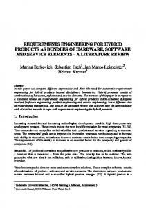
2 Background 2.1 The Four Variable Model The Four Variable Model, which is illustrated in Figure 1, describes the required system behavior as a set of mathematical relations on four sets of variables| monitored and controlled variables and input and output data items. A monitored variable represents an environmental quantity that in uences system behavior, a controlled variable an environmental quantity that the system controls. Input devices (e.g., sensors) measure the monitored quantities and output devices set the controlled quantities. The variables that the devices read and write are called input and output data items. The four relations of the Four Variable Model are REQ, NAT, IN, and OUT. The relations REQ and NAT provide a black box speci cation of the required

Form Approved OMB No. 0704-0188

Report Documentation Page

Public reporting burden for the collection of information is estimated to average 1 hour per response, including the time for reviewing instructions, searching existing data sources, gathering and maintaining the data needed, and completing and reviewing the collection of information. Send comments regarding this burden estimate or any other aspect of this collection of information, including suggestions for reducing this burden, to Washington Headquarters Services, Directorate for Information Operations and Reports, 1215 Jefferson Davis Highway, Suite 1204, Arlington VA 22202-4302. Respondents should be aware that notwithstanding any other provision of law, no person shall be subject to a penalty for failing to comply with a collection of information if it does not display a currently valid OMB control number.

1. REPORT DATE

3. DATES COVERED 2. REPORT TYPE

1996

00-00-1996 to 00-00-1996

4. TITLE AND SUBTITLE

5a. CONTRACT NUMBER

Requirements Specifications for Hybrid Systems

5b. GRANT NUMBER 5c. PROGRAM ELEMENT NUMBER

6. AUTHOR(S)

5d. PROJECT NUMBER 5e. TASK NUMBER 5f. WORK UNIT NUMBER

7. PERFORMING ORGANIZATION NAME(S) AND ADDRESS(ES)

Naval Research Laboratory,Code 5546,4555 Overlook Avenue, SW,Washington,DC,20375 9. SPONSORING/MONITORING AGENCY NAME(S) AND ADDRESS(ES)

8. PERFORMING ORGANIZATION REPORT NUMBER

10. SPONSOR/MONITOR’S ACRONYM(S) 11. SPONSOR/MONITOR’S REPORT NUMBER(S)

12. DISTRIBUTION/AVAILABILITY STATEMENT

Approved for public release; distribution unlimited 13. SUPPLEMENTARY NOTES 14. ABSTRACT 15. SUBJECT TERMS 16. SECURITY CLASSIFICATION OF:

17. LIMITATION OF ABSTRACT

a. REPORT

b. ABSTRACT

c. THIS PAGE

unclassified

unclassified

unclassified

18. NUMBER OF PAGES

19a. NAME OF RESPONSIBLE PERSON

11

Standard Form 298 (Rev. 8-98) Prescribed by ANSI Std Z39-18

Environment

Monitored Variables

Input Data Input Items Devices

System

IN

Software

Output Data Items

Output Devices

SOFT

Controlled Variables

Environment

OUT

REQ and NAT

Fig. 1.

Four Variable Model.

system behavior. NAT describes the natural constraints on system behavior| that is, the constraints imposed by physical laws and by the system environment. REQ de nes the system requirements as a relation the system must maintain between the monitored and the controlled quantities. One approach to describing the required system behavior, REQ, is to specify the ideal system behavior, which abstracts away timing delays and imprecision, and then to specify the allowable system behavior, which bounds the timing delays and imprecision. Typically, a function speci es ideal system behavior, whereas a relation speci es the allowable system behavior. The allowable system behavior is a relation rather than a function because it may associate a monitored variable with more than a single value of a controlled variable. For example, if the system is required to display the current water level, it may be acceptable for the displayed value of water level at time t to deviate from the actual value at time t by as much as 0.1 cm. The system requirements are easier to specify and to reason about if the ideal behavior is de ned rst. Then, the required precision and timing can be speci ed separately. This is standard engineering practice. Moreover, this approach provides an appropriate separation of concerns, since the required system timing and accuracy can change independently of the ideal behavior [3]. The relation IN speci es the accuracy with which the input devices measure the monitored quantities and the relation OUT speci es the accuracy with which the output devices set the controlled quantities. To achieve the allowable system behavior, the input and output devices must measure the monitored quantities and set the controlled quantities with sucient accuracy and suciently small timing delays. In the Four Variable Model, the software requirements speci cation, called SOFT, de nes the required relation between the input and output data items. SOFT can be derived from REQ, NAT, IN, and OUT.

2.2 SCR Requirements Speci cations

The SCR requirements method was introduced in 1978 with the publication of the requirements speci cation for the A-7 Operational Flight Program [10, 1]. Since its introduction, the method has been extended to specify system as well as software requirements and to include, in addition to functional behavior, the required system timing and accuracy [12, 13, 14]. Designed for use by engineers,

Pressure

{

Mode Class

High

Permitted

Safety Injection System WaterPres Block Environment Reset

Sensor1

Input Devices Sensor2 Sensor3

Fig. 2.

{

Terms

TooLow

Overridden .

Safety Injection Device

Software Display Device

. .

Output Output Devices Devices

Safety Injection

Environment Display Pres

Requirements Speci cation for Safety Injection.

the SCR method has been successfully applied to a variety of practical systems, including avionic systems; a submarine communications system [9]; and safetycritical components of a nuclear power plant [14]. More recently, a version of the SCR method called CoRE [4] was used to document requirements of Lockheed's C-130J Operational Flight Program (OFP) [5]. The OFP consists of more than 100K lines of Ada code, thus demonstrating the scalability of the SCR method. To represent requirements both abstractly and concisely, SCR speci cations use two special constructs, called mode classes and terms. A mode class is a state machine, de ned on the monitored variables, whose states are called system modes (or simply modes) and whose transitions are triggered by changes in the monitored variables. Complex systems are de ned by several mode classes operating in parallel. A term is an auxiliary function de ned on monitored variables, mode classes, or other terms. In SCR speci cations, conditions and events are used to describe the system states. A condition is a logical proposition de ned on a single system state, whereas an event is a logical proposition de ned on a pair of system states. An event occurs when a system entity (that is, a monitored or controlled variable, a mode class, or a term) changes value. A special event, called an monitored event, occurs when a monitored variable changes value. Another special event, called a conditioned event, occurs if an event occurs when a speci ed condition is true. To illustrate the SCR method, we consider a simpli ed version of the control system for safety injection described in [2]. The system uses three sensors to monitor water pressure and turns on a safety injection system (which adds coolant to the reactor core) when the pressure falls below some threshold. The system also displays the current value of water pressure. The system operator blocks safety injection by turning on a \Block" switch and resets the system after blockage by turning on a \Reset" switch. Figure 2 shows how SCR constructs are used in specifying the requirements of the control system. Water pressure and the \Block" and \Reset" switches are represented as monitored variables, WaterPres, Block, and Reset; safety injection and the display as controlled variables, SafetyInjection and DisplayPres; each sensor value as an input data item; and the hardware interfaces between the control system software and the safety injection system and the display output as output data items. The speci cation for the control system includes a mode class Pressure, a term Overridden, and several conditions and events. The mode class Pressure,

Old Mode

TooLow Permitted Permitted High Table 1.

Event

@T(WaterPres  Low) @T(WaterPres  Permit) @T(WaterPres < Low) @T(WaterPres < Permit)

New Mode

Permitted High TooLow Permitted

Mode Transition Table for Pressure.

Mode

Events

High TooLow, Permitted Overridden

False @T(Block=On) WHEN Reset=Off True

Table 2.

@T(Inmode) @T(Inmode) OR @T(Reset=On) False

Event Table for Overridden.

an abstract model of the monitored variable WaterPres, contains three modes, TooLow, Permitted, and High. At any given time, the system must be in one of these modes. A drop in water pressure below a constant Low causes the system to enter mode TooLow; an increase in pressure above a larger constant Permit causes the system to enter mode High. The term Overridden denotes situations in which safety injection is blocked. An example of a condition in the speci cation is \WaterPres < Low". Events are denoted by the notation \@T". Two examples of events are the monitored event @T(Block=On) (the operator turns Block from Off to On) and the conditioned event @T(Block=On) WHEN WaterPres < Low (the operator turns Block to On when water pressure is below Low). SCR requirements speci cations use special tables, called condition tables, event tables, and mode transition tables, to represent the required system behavior precisely and concisely. Each table de nes a mathematical function.1 A condition table describes a controlled variable or a term as a function of a mode and a condition; an event table describes a controlled variable or term as a function of a mode and an event. A mode transition table describes a mode as a function of another mode and an event. While condition tables de ne total functions, event tables and mode transition tables may de ne partial functions, because some events cannot occur when certain conditions are true. For example, in the control system above, the event @T(Pressure=High) WHEN Pressure=TooLow cannot occur, because starting from TooLow, the system can only enter Permitted when a state transition occurs. Tables 1{3 are part of REQ, the requirements speci cation for the control system. Table 1 is a mode transition table describing the mode class Pressure as 1

Although SCR speci cations can be nondeterministic, our initial model is restricted to deterministic systems.

Mode

Conditions

High, Permitted

True

TooLow

Overridden

NOT Overridden

Safety Injection

Off

On

Table 3.

Condition Table for Safety

False

Injection.

a function of the current mode and the monitored variable WaterPres. Table 2 is an event table describing the term Overridden as a function of Pressure, Block, and Reset. Table 3 is a condition table describing the controlled variable Safety Injection as a function of Pressure and Overridden. Table 3 states, \If Pressure is High or Permitted, or if Pressure is TooLow and Overridden is true, then Safety Injection is Off; if Pressure is TooLow and Overridden is false, then Safety Injection is On."2

3 SCR Requirements Model To provide a formal foundation for tools analyzing the speci cations and simulating system execution [7, 6], we have developed a discrete version of the Four Variable Model, called the SCR requirements model [8]. The SCR model represents a system as a nite state machine and each monitored and controlled quantity as a discrete variable. Presented below are excerpts from the de nition of the formal model [8] and a description of the interpretation of the REQ and NAT relations within the SCR model.

3.1 Summary of the SCR Model Entities and Types. We require the following sets. { { { {

MS is the union of N nonempty, pairwise disjoint sets, M1 ; M2 ; : : : ; MN , called mode classes. TS is a union of data types, where each type is a nonempty set of values.3 VS is a set of entity values with VS = MS [ TS. RF is a set of entity names r, which is partitioned into the set of mode names MR, the set of monitored variable names IR, the set of term names GR, and the set of controlled variable names OR. For all r 2 RF, TY(r)  VS is the type (i.e., the set of possible values) of entity r.

System State and Conditions. A system state s is a function that maps each entity name r in RF to a value. That is, for all r 2 RF: s(r) = v, where v 2 TY(r). Conditions are logical propositions de ned on entities in RF. 2

The notation \@T(Inmode)" in a row of an event table describes system entry into the group of modes in that row. 3 For example, the type \nonnegative integers" is the set N = f0; 1; 2; : : :g, the type Boolean is the set B = ft rue; f alseg, etc.

System and Events. A system is a state machine whose transition from one

state to the next is triggered by special events, called monitored events. More precisely, a system, , is a 4-tuple  = (E m ; S; s0 ; T); where {

{ { {

E m is a set of monitored events. A primitive event is denoted as @T(r = v), where r 2 RF is an entity and v 2 TY(r). A monitored event is a primitive event @T(r = v), where r 2 IR is a monitored variable. S is the set of possible system states. s0 is a special state called the initial state. T is the system transform, a function from E m  S into S .

In addition to denoting primitive events, the \@T" notation also denotes conditioned events. A simple conditioned event is expressed as @T(c) WHEN d; where @T(c) is any event (i.e., a change in a state variable) and d is a simple condition or a conjunction of simple conditions. A conditioned event e is a logical proposition composed of simple conditioned events connected by the logical connectors ^ and _. The proposition represented by a simple conditioned event is de ned by @T(c) WHEN d = NOT c ^ c ^ d; where the unprimed version of c represents c in one state (the old state) and the primed version of c represents c in another state (the new state). System History Associated with every monitored variable r 2 IR is a set of ordered pairs Vr , Vr = f(v; v ) j v 6= v ; v 2 TY(r); v 2 TY(r)g; that de nes all possible transitions of r and that contains r's initial value. A monitored event @T(r = v ) is enabled in state s if (s(r); v ) 2 Vr . A history  of a system is a function from the set of nonnegative integers N to E m  S such that (1) the second element of (0) is s0 , (2) for all n 2 N , if (n) = (e; s), then e is enabled in s, and (3) for all n 2 N , if (n) = (e; s) and (n+1) = (e ; s ), then T(e; s) = s . Ordering the Entities. Given an input event e in Em , states s and s in S, and T(e; s) = s , the value of each entity r in state s may depend on any entity in the old state s but on only some entities in the new state s . To describe the dependencies of any entity r 2 RF on entities in the new state, we order the entities in RF as a sequence R, R = ; where < r1; r2; : : :; rI >; ri 2 IR, is the subsequence of monitored variables, ; ri 2 GR [ MR, is the subsequence containing terms and modes, and < rK +1 ; rK +2; : : :; rP >; ri 2 OR is the subsequence of controlled variables. 0

0

0

0

0

0

0

0

0

0

0

0

0

Modes

Conditions

m1 m2 ::: mn ri Table 4.

c1;1 c2;1 ::: cn;1 v1

c1;2 c2;2 ::: cn;2 v2

::: ::: ::: ::: :::

c1;p c2;p ::: cn;p vp

Typical Format for a Condition Table.

The entities ri 2 R are partially ordered so that for all i, i , i > I, 1  i  K; the value of entity ri in any state s can only depend on the value of entity ri in the same state s if i < i. This de nition re ects the fact that each monitored variable can only be changed by external events and cannot depend on the other entities in R. In contrast, each term in s can depend on the monitored variables, the modes, or other terms in s. Similarly, each mode in s can depend on the monitored variables, the terms, or other modes in s. Finally, each controlled variable in s can depend on any entity that precedes it in the sequence R. Computing the Transform Function. Each controlled variable, term, and mode class ri 2 RF n IR is de ned by a function Fi. The transform function T computes the new state by composing the Fi 's. In an SCR requirements speci cation, most of the Fi 's are described by tables. Table 4 shows a typical format for one class of tables, condition tables. A condition table describes an output variable or term ri as a relation i , i = f(mj ; cj;k; vk ) 2 M(i)  Ci  TY(ri ) j 1  j  n; 1  k  pg; where Ci is a set of conditions de ned on entities in RF and M(i) is the mode class associated with ri . The relation i must satisfy the following properties: 0

0

0

0

1. 2. 3.

The mj and the vk are unique.

[ni=1 mj = Mp (i) (All modes in the mode class are included). For all j : _k=1 cj;k = true ( The disjunction of the conditions in each Coverage:

row of the table is true). 4. For all j; k; l; k 6= l: cj;k ^ cj;l = false (Disjointness: The pairwise conjunction of the conditions in each row of the table is always false).

Given these properties, we can show that i is a function, which can be expressed as: for all j; k; 1  j  n; 1  k  p, i (mj ; cj;k ) = vk . To make explicit entity ri's dependencies on other entities, we consider an alternate form Fi of the function i . To de ne Fi, we require the new state dependencies set, fyi;1; yi;2; : : :; yi;n g, where yi;1 is the entity name for the associated mode class and for all j, 2  j  ni , yi;j appears in some condition c in Ci. i

Based on this set and i , we de ne Fi as

8 v1 if (yi;1 = m1 ^ c1;1 ) _ : : : _ (yi;1 = mn ^ cn;1) >< v2 if (yi;1 = m1 ^ c1;2 ) _ : : : _ (yi;1 = mn ^ cn;2) Fi(yi;1 ; yi;2 ; : : : ; yi;n ) = > .. : .vp if (yi;1 = m1 ^ c1;p ) _ : : : _ (yi;1 = mn ^ cn;p ): i

The four properties guarantee that Fi is a total function.

3.2 The SCR Model, REQ, and NAT NAT. In the SCR model, NAT models the behavior of the monitored and controlled quantities. Consider the monitored variable Block in the example above and let m = Block. The type de nition of m is TY(m ) = fOff, Ong and the possible changes of m from one state to the next are de ned by Vm1 = f(Off, On); (On, Off)g; that is, Block can change from Off to On or from On to Off. Similarly, for the monitored variable m = Reset and the controlled variable c = SafetyInjection, TY(m ) =TY(c ) = fOff, Ong and Vm2 = Vc1 = f(Off, On); (On, Off)g. 1

1

1

1

2

1

2

1

The current SCR model describes all monitored and controlled quantities, even those which are naturally continuous, as discrete variables. Doing so allows us to represent the system as a nite state machine. This representation facilitates formal analysis of the speci cations and symbolic execution of the system via simulation. For example, to model WaterPres as a discrete variable, we assign m3 = WaterPres the type de nition TY (m3 ) = f14; 15; : : :; 2000g, that is, m3 is any integer between 14 and 2000. We constrain changes in WaterPres by requiring that WaterPres can change from one state to the next by no more than 1 psi, that is, js (m3 ) , s(m3 )j 2 f0; 1g; where s and s are any two consecutive states. This assumption implies the statement in Section 2.2 that the mode class Pressure cannot transition directly from TooLow to High or from High to TooLow. Similarly, we can de ne the type of controlled variable c2 = DisplayPres as TY (c2 ) = f14; 15; : : :; 2000g and constrain changes in c2 by requiring that, if s and s are any two consecutive states, then js (c2 ) , s(c2 )j 2 f0; 1g. Ideal Behavior. In the SCR model, the transform function T de nes the ideal system behavior. As noted above, T computes the new state from an event and the current state by composing the functions Fi that de ne the values of terms, mode classes, and controlled variables. Clearly, reasoning about the ideal system behavior using T abstracts away timing delays and imprecision. 0

0

0

0

4 Extending the SCR Model to Hybrid Systems To use the SCR model to specify and to reason about hybrid systems, we need to extend the model in two ways:

{ Each monitored quantity and controlled quantity that is naturally continuous is represented by a continuous (rather than a discrete) variable. { The allowable system behavior is de ned by associating timing and accuracy requirements with each controlled variable.

4.1 Adding Continuous Variables As an example, consider the monitored variable m3 = WaterPres and the controlled variable c2 = DisplayPres. We can de ne m3 as a real number between 14.0 and 2000.0, that is, TY(m3 ) = fx j x 2 R+ ^ 14:0  x  2000:0g. Physical laws (part of NAT) bound the rate at which m3 can change. To express this bound, we may state in the speci cation that, in any time interval of length 0.1 seconds, the maximum change in the value of WaterPres is 0.03 psi; that is, jm3 (t ) , m3 (t)j  :03; when t , t = 0:1 sec. The constraints on c2 may be de ned in a similar way. Clearly, the bounds can be expressed by more complex functions, e.g., by continuously dierentiable functions, by piecewise continuous functions, or by bounded derivatives. We note that any reasoning that used the discrete models of WaterPres and DisplayPres to analyze system behavior should be reevaluated to make sure the reasoning is still valid when more accurate models of these two naturally continuous quantities are used. This is especially important when discrete approximations of continuous quantities are used in verifying critical system properties. 0

0

4.2 Adding Time The SCR model introduced in Section 3.1 is untimed. Thus if an event occurs in state s that changes a controlled variable, we assume that the next state s re ects the change in the controlled variable (as well as changes in the monitored variable that triggered the new state and any resulting changes in mode classes, terms, and other controlled variables). To add time to the SCR model, we adapt the approach developed by Lynch and Vaandrager [11] for timed automata. This approach associates each event in a state history with a time. More precisely, for each state history, s0 ; (e1; s1 ); (e2; s2 ); : : :, we de ne a sequence of the form (e1 ; t1); (e2; t2 ); : : :, where each ei is either a monitored event or an event changing the value of a controlled variable and each ti is a non-negative real-valued time. We require that, for all i, i + 1, ti+1  ti and de ne a function TIME that maps each event e in a system history to a time t, that is, TIME(e) = t. 0

4.3 Specifying the Actual System Behavior To specify the allowable system behavior, we associate timing and accuracy requirements with each controlled variable. Consider, for example, the controlled

variable DisplayPres in the example, and let c2 = DisplayPres. To specify the constraints on c2, we must state the degree of accuracy that is required in the displayed value of WaterPres. For example, we may require that the displayed value of WaterPres at any given t is within 0.1 psi of the actual value of WaterPres at time t, that is, jc2(t) , m3 (t)j  0:1 psi. Consider a system design that uses a given input device to measure WaterPres, a given output device to write the value of WaterPres to the display, and speci c hardware and software. Then, the maximum rate at which WaterPres can change in a given time interval (de ned by NAT), the degree of accuracy and timing delays associated with the input and output devices (de ned by IN and OUT), and the system delay in reading from and writing to the devices together determine whether the required accuracy can be achieved. To specify the requirements for turning the safety injection system on and o, we must specify timing constraints on the controlled variable SafetyInjection. Let c1 represent SafetyInjection. Suppose that the safety injection system must be turned on within, say, 0.2 seconds after the occurrence of the triggering event (e.g., WaterPres drops below Low when Overridden= false). Then, if the triggering event ek occurs at time t, that is, TIME(ek ) = t, the event ek+j that turns on SafetyInjection must occur within the time interval [t; t + 0:2], that is, TIME(ek+j ) 2 [t; t + 0:2]. By considering a particular system design|that is, the timing delays and degree of accuracy of the input and output devices and computer hardware and software that control safety injection|we can compute whether safety injection will always be activated within the required time interval.

5 Summary We have presented several examples to show how the SCR requirements model can be extended to specify and to reason about hybrid systems. The next step is to extend the formal de nition of the SCR model to include continuous variables, time, and accuracy. By adding such information to system and software requirements speci cations, we can provide precise guidance to the developers of computer systems and a formal foundation for analyzing the behavior of these systems.

Acknowledgments The perceptive and constructive comments of Stuart Faulk, Ralph Jeords, Jim Kirby, and Bruce Labaw on an earlier draft are gratefully acknowledged.

References 1. Thomas A. Alspaugh, Stuart R. Faulk, Kathryn Heninger Britton, R. Alan Parker, David L. Parnas, and John E. Shore. Software requirements for the A-7E aircraft. Technical Report NRL-9194, Naval Research Lab., Wash., DC, 1992. 2. P.-J. Courtois and David L. Parnas. Documentation for safety critical software. In Proc. 15th Int'l Conf. on Softw. Eng. (ICSE '93), pages 315{323, Baltimore, MD, 1993. 3. Stuart Faulk, Lisa Finneran, James Kirby, Jr., and Assad Moini. Consortium requirements engineering handbook. Technical Report SPC-92060-CMC, Software Productivity Consortium, Herndon, VA, December 1993. 4. Stuart R. Faulk, John Brackett, Paul Ward, and James Kirby, Jr. The CoRE method for real-time requirements. IEEE Software, 9(5):22{33, September 1992. 5. Stuart R. Faulk, Lisa Finneran, James Kirby, Jr., S. Shah, and J. Sutton. Experience applying the CoRE method to the Lockheed C-130J. In Proc. 9th Annual Conf. on Computer Assurance (COMPASS '94), pages 3{8, Gaithersburg, MD, June 1994. 6. Constance Heitmeyer, Alan Bull, Carolyn Gasarch, and Bruce Labaw. SCR*: A toolset for specifying and analyzing requirements. In Proc. 10th Annual Conf. on Computer Assurance (COMPASS '95), pages 109{122, Gaithersburg, MD, June 1995. 7. Constance Heitmeyer, Bruce Labaw, and Daniel Kiskis. Consistency checking of SCR-style requirements speci cations. In Proc., International Symposium on Requirements Engineering, March 1995. 8. Constance L. Heitmeyer, Ralph D. Jeords, and Bruce G. Labaw. Tools for analyzing SCR-style requirements speci cations: A formal foundation. Technical Report NRL-7499, Naval Research Lab., Wash., DC, 1995. In preparation. 9. Constance L. Heitmeyer and John McLean. Abstract requirements speci cations: A new approach and its application. IEEE Trans. Softw. Eng., SE-9(5):580{589, September 1983. 10. Kathryn Heninger, David L. Parnas, John E. Shore, and John W. Kallander. Software requirements for the A-7E aircraft. Technical Report 3876, Naval Research Lab., Wash., DC, 1978. 11. Nancy Lynch and Frits Vaandrager. Forward and backward simulations for timingbased systems. In Proceedings of REX Workshop \Real-Time: Theory in Practice", volume 600 of Lecture Notes in Computer Science, pages 397{446, Mook, The Netherlands, June 1991. Springer-Verlag. 12. David L. Parnas and Jan Madey. Functional documentation for computer systems. Technical Report CRL 309, McMaster Univ., Hamilton, ON, Canada, September 1995. 13. A. John van Schouwen. The A-7 requirements model: Re-examination for real-time systems and an application for monitoring systems. Technical Report TR 90-276, Queen's Univ., Kingston, ON, Canada, 1990. 14. A. John van Schouwen, David L. Parnas, and Jan Madey. Documentation of requirements for computer systems. In Proc. RE'93 Requirements Symp., pages 198{207, San Diego, CA, January 1993. This article was processed using the LATEX macro package with LLNCS style