trade crude grain money-supply interest ship sugar money-fx no. of docs 441 ..... which is the cluster type divided by the overall number .... time scales with n3.
Resampling methods for document clustering D. Volk1 and M.G. Stepanov1,2
arXiv:cond-mat/0109006v1 [cond-mat.dis-nn] 1 Sep 2001
1
Physics of Complex Systems, Weizmann Institute of Science, Rehovot 76100, Israel 2 Institute of Automation and Electrometry, Novosibirsk 630090, Russia
We compare the performance of different clustering algorithms applied to the task of unsupervised text categorization. We consider agglomerative clustering algorithms, principal direction divisive partitioning and (for the first time) superparamagnetic clustering with several distance measures. The algorithms have been applied to test databases extracted from the Reuters-21578 text categorization test database. We find that simple application of the different clustering algorithms yields clustering solutions of comparable quality. In order to achieve considerable improvements of the clustering results it is crucial to reduce the dictionary of words considered in the representation of the documents. Significant improvements of the quality of the clustering can be obtained by identifying discriminative words and filtering out indiscriminative words from the dictionary. We present two methods, each based on a resampling scheme, for selecting discriminative words in an unsupervised way. Keywords: clustering, text categorization, document classification, feature selection, random subsampling
engine and a clustering tool has been proposed e. g. by Boley [3]. The aims of this work are threefold. First we want to compare several methods measuring their performance on unsupervised text categorization. Second we want to apply superparamagnetic clustering (SPC) [4,5], a rather new method that has so far not been considered for text categorization. And third we want to present two methods of unsupervised feature selection and estimate the improvements that can be achieved by their application.
I. INTRODUCTION
Automatic text categorization has many interesting applications in science and business. For instance formatting the results of a web-search query, sorting news messages according to topics or sorting incoming email with different concerns. Irrespective of the application two principal cases are distinguished. In the first case the categories are known and the algorithm should assign any document to one of the known categories. Then it is useful to teach the algorithm the considered categories and their word fields by using a training set of labeled documents before it will be applied to unknown documents. The algorithmic solutions to this problem fall into the category of supervised learning. In the other case the categorization of documents has to be done without knowing the categories nor their number. Then the algorithm should find a reasonable partition of the document set such that documents in the same subset of the partition are similar and documents of different subsets are dissimilar. This task is termed unsupervised text categorization and can be handled with clustering algorithms [1,2]. In this work we focus on the second task only. As an illustrative example for an application one could think of the results obtained from web search engines. Usually the query results are on several subjects and only a fraction of the documents is about what one is interested in. It will help the user if instead of an unsorted list the results are presented in several folders that gather webdocuments of similar content. Further each folder could be characterized by a list of key words. Then one can investigate the mass of documents that match a query in a more efficient way and the indicated keywords may help refining the search. In the general case of web search results we are not supplied with any training data such that we can only use clustering algorithms in order to classify the links. Such a combination of a web search
II. CLUSTERING ALGORITHMS
Clustering of data is usually done in three steps: representation, calculation of similarities and application of a clustering algorithm. As mentioned above the aim is to provide a partition of a data set X that reflects the similarities between data points. So we should define a similarity measure s : X × X → R which in turn requires a numerical representation of the data. Usually the representation is done by constructing a vector space spanned by a set of selected features of the data. This means that one defines certain features and for all data assigns numbers according to how much the features apply. Then a data point is represented by a vector in the feature space. For text categorization one commonly uses the “bag of words” representation. In order to do so one enlists a dictionary W = {w1 , w2 , . . . , wm } of all the words that appear at least once in at least two of the documents. Documents are then represented by counting the number of occurrences of each word in the document. One thus obtains an n × m-matrix F = (fαi ) of word frequencies. fαi is the number of times the word wi appears in document xα and document xα is represented by the feature (row-)vector (fαi )i=1,...,m . Typically that feature space is very high-dimensional and the matrix is filled 1
For practical purposes it is then often important to reduce the amount of information in the tree, and present only some selected clusters as the essence of the clustering. Then one can apply a search algorithm that selects the “most meaningful” clusters in the tree for presentation as the clustering result. Applying an algorithm that searches a tree for good clusters can be considered the fourth step of clustering and can be done in various ways. When one is using SPC one can look at the change of the susceptibility versus the temperature and from that function one can determine the “best” resolution [4]. But the search is not restricted to finding an optimal single resolution. For the text categorization task we found that the natural classes of the documents as classified by human readers, and so specified by the labels, are best approximated at different levels of resolution. Therefore we prefer other methods that individually judge a single cluster as good or bad and therefore allow picking clusters from different levels of resolution. This can be done by measuring the stability of the cluster with respect to the resolution parameter [7] or with respect to thinning out the dataset by considering subsamples [8]. However, the unsupervised identification of good clusters is a complex issue that we do not discuss in this paper, cp. section IV C.
very sparsely, in our case the fraction of nonzero entries is ≈ 2%. To measure the similarity of two documents one could consider for instance the dot product of two corresponding normalized feature vectors. Alternatively one can of course use a dissimilarity measure. The choice of the similarity measure has to be done carefully and influences the performance of the clustering. See e.g. [6] for a comparison of some similarity measures used for text categorization. For the text categorization we found useful the l1 - and l2 -norms as well as other dissimilarity measures (see below). Generally, in order to avoid skewness of the data due to the different length of the documents, it is helpful to normalize the data such that the length of a row vector is one. Finally, given the similarity measure s the task of a clustering algorithm is to compute a clustering solution, i.e. a partition of the set of data points X into subsets (clusters) {C1 , C2 , . . . , Cn } such that s(xα , xβ ) is large when xα and xβ are in the same cluster and s(xα , xβ ) is small when xα and xβ are in different clusters. This is a rather fuzzy description of the aim of a clustering algorithm and we are not going to refine that point here. A good clustering solution can be found at different resolutions, so that a proper optimization problem can not easily be formulated. Consider for example the biological classification of the animals. There we find phyla that are further subdivided into classes, orders, etc. and each level of partitioning has some justification. If we consider a clustering of the animals cat, dog, jellyfish, mouse and snake, we find dog and cat in the same cluster but well separated from the jellyfish when we a take a look from a large distance and consider a coarse classification. A finer classification however will separate dog and cat into different clusters. For many data sets this resolution is an arbitrary parameter which has to be determined in accordance with the desired classification task. We therefore do not consider a single partition of the data set as a clustering solution but rather a hierarchy of partitions with increasing resolution that can be represented in a tree. Agglomerative clustering methods [2] successively merge two clusters until finally all data points are united. By doing so these methods implicitly provide such a tree. SPC and k-means provide single partitions which depend on a resolution parameter that has to be specified. Running these algorithms with different values of the resolution parameter yields several partitions that can be transformed into a tree. Generally the partitions obtained at the next higher resolution are not proper subpartitions. In order to fix this one usually considers the intersections of high resolution clusters and low resolution clusters. Each triplet of a representation, a distance measure and a clustering algorithm is considered as a clustering method. In section IV we specify in detail the methods we apply to the test data. All methods we compare yield a hierarchical clustering tree.
III. FEATURE SELECTION: FINDING DISCRIMINATIVE WORDS
A crucial point within the representation of the documents that bears some potential to improve the clustering results is the selection of words from the dictionary. Everybody will immediately agree that the words “and”, “or”, “while” and “with” are useless for document categorization. These words are not characteristic for the content of the document and spoil the signal to noise ratio in the representation. Usually words like prepositions, conjunctions, etc. are read from a stoplist that contains about 400 known stopwords. They are taken out of the dictionary, i.e. out of the feature set and, as we will show in our results, this rejection of unwanted features yields some improvement on the results. So far this is not new, but this procedure, however, does only a part of the job. A more difficult problem is to get rid of those many noise words that are not on the stoplist. After the application of the stoplist we remain with 5036 and 9019 words respectively to our two test databases. On the other hand, looking at the DSR experiments that are described below, we find improved clustering results on the basis of 350 automatically selected words. So more than 90% of the words that are not on the stoplist are not needed. More than that: they make the task harder because they add noise to the document representation. 2
Hi = − (pi1 log pi1 + pi2 log pi2 ) ,
Finding those good words is not easy. Whether a word is a useful feature for document classification depends on the categories that appear in the document set and can not be told by looking at the mere word. The word “Italy” for instance might be discriminative in some set of documents where one of the categories is tourism, but it can be a pure noise feature in another set of documents. A widely used method is the application of lower and upper thresholds for the coverage of a word, i.e. the number of documents a word appears in. This can improve the results but the quality of the clustering depends sensitively on these thresholds and one can not tell in general which values of these thresholds are the best. An alternative way to select relevant features, that has been proven useful for the analysis of microarray data, is the application of clustering algorithms to the feature set [7]. In order to identify good words and throw away the bad words in an unsupervised way we developed two strategies that are both based on resampling.
where {xα |fαi > 0} ∩ Cj
, pij = {xα |fαi > 0} ∩ (C1 ∪ C2 )
j = 1, 2.
(4)
Further, at that stage we check for each pair of documents if they are in the same cluster: � 1, if xα , xβ are in the same cluster; (5) Mαβ = 0, otherwise. We repeat this probe clustering until we have NR “good” ones. The word subsets are obtained by throwing out one randomly drawn word from each document. In order to avoid empty documents in some cases some of the thrown out words have to be replaced. After doing all subsample clusterings we average Hi and Mαβ over all NR “good” probe clusterings. Intuitively we consider hHi i as the quality of the word wi , and hMαβ i as similarity of the documents xα and xβ (h...i denotes average). We throw away all the words whose average entropy exceeds the threshold:
A. Word set resampling (WSR)
Experiments with different thresholds for minimal and maximal coverage have shown that choosing a different word subset for clustering the same database can strongly affect the global clustering tree structure. Such sensitivity is probably due to “shot noise” arising from the finite size of the dictionary (and an even smaller number of words that appear in a single category or a single document). One way to eliminate such noise is taking different, e.g. randomly chosen, word subsets from the dictionary, clustering the documents on the basis of these subsets and then averaging the result somehow. This is the idea of the word set resampling algorithm described in the following. Let us first explain the procedure that is applied for each word subset (“probe clustering”). We cluster the documents represented only through the words in the subset by applying an agglomerative clustering algorithm (see below). Each agglomeration process is continued until the stop criterion (1) holds [16], where C1 and C2 are the two largest clusters and |C2 | < |C1 |: � � 1 |X|. (1) |C1 | + |C2 | ≥ 1 − e
hHi i > θ log 2,
(6)
where θ ∈ [0, 1]. Next, we find the maximal value M = maxα6=β hMαβ i and merge together all the documents xα , xβ with hMαβ i = M . In the next step we remove all the words that appear solely in documents of one cluster. Unless we are left with one huge cluster of all the documents we will repeat this procedure. In doing so we consider as single documents in the next step those that were merged in the current step. The parameters of this algorithm are NR and θ. B. Document set resampling (DSR)
This method is motivated by the good results obtained with WSR. It is meant to be an alternative that does not require such a high computing time as WSR. Whereas WSR calculates the entropy of the words only at a single stage of the subsample clustering, DSR tries to get hints for the good words by looking at the whole clustering of the subsamples. DSR is based on two assumptions that have been found to be true in our experiments: first we found that the really useful words have a considerable coverage, i. e. these words appear in many documents. Second we assume that in agglomerative clustering, when we consider the number of mergings that have been done as a monotonically decreasing measure of the clustering resolution, the cluster entropy of the good words often decreases earlier
The clustering is then considered as “good” if the following quality condition is not violated. |X| − |C1 | − |C2 | < |C2 |.
(3)
(2)
One can see that if both conditions (1) and (2) hold, then C1 , C2 are of comparable size and contain the majority of the documents (there is no other aim of (1) and (2)). If the probe clustering is not “good” then it is rejected. For “good” clusterings we calculate for every word the entropy with respect to the two biggest clusters: 3
that is significantly higher than the average increment as a cutoff criterion at which we decide to keep the words that have low entropy according to (13) at that stage. (k) That is we look for the minimal value r∗ fulfilling q
� (k) ∆(k) (r∗ ) > h∆(k) i + (12) (∆(k) − h∆(k) i)2
with decreasing resolution than the cluster entropy of the bad words. The detailed description of the algorithm is as follows: We create NR subsamples X (k) ⊂ X, k = 1, . . . , NR , each consisting of nsub randomly drawn documents. To each subset X (k) we apply an agglomerative clustering algorithm. We number the successive mergings of the agglomeration and we will refer to the intermediate clustering solutions at step r. By r = 1 we refer to the initialization with each single document being in a separate cluster and r = nsub corresponds to the final step where all documents are in a single cluster. We then consider the words that appear in at least nmin documents of the current subsample and for each of these words we calculate the development of its cluster entropy in the early steps of the agglomeration process, i.e. r = 1, 2, . . . , 0.7nsub . Thus at step r we find the clusters Cl with the labels l ∈ Lr = {1, . . . , nsub − r + 1} and we calculate X ˜ (k) (r) = − P (k) (l|wi ) log P (k) (l|wi ) (7) H i
and we select good words as (k)
P
(l|wi ) =
α∈Cl
fαi
,
X
fαi .
IV. COMPARISON OF THE CLUSTERING METHODS A. The test dataset and the different experiments
α∈X (k)
In order to compare the performance of the different clustering algorithms we extracted two test data sets from the known Reuters-21578 test database for text categorization [9]. This database contains 21578 Reuters news messages that were manually labeled as belonging to certain categories. We use the labels not for the clustering procedure but in order to evaluate the quality of the clustering results as will be described in the next section. For each of our two test datasets we took all documents of eight selected categories. In order to keep things simple we considered some preprocessing of the labels as helpful. Those few documents that have been labeled as belonging to more than one category were assigned unambiguously to the first label given in the database. One should keep in mind that the labels were given by human readers and are therefore subject to individual perception. The resulting test databases, i.e. the categories that are to be separated from one another and the number of documents extracted from the Reuters database are listed in table I. Please note that some categories appear in both tasks. This is meant as shedding some light onto whether the good or bad separability of a category is an individual property of that category and its word field or if it rather a question of interference with another category using the same words. We found that the quality of clustering results is sensitive to the input dataset, particularly to the composition of the news categories that are used. For instance, in clustering experiments done with the first database all clustering algorithms separate documents of the category
In order to highlight the effect of successive mergings on the cluster entropy we normalize the cluster entropies with respect to the initial cluster entropies at step r = 1 (9)
(k)
Now Hi (r) decreases as the resolution becomes lower with successive mergings, i.e. as r increases, and finally, when all documents have been merged to the same cluster the entropy is zero for all words. We found that if we consider only the words the entropy of which decreases early in the agglomeration process we find a higher fraction of good words that have more value for the document clustering. However, the entropy of words that appear only in two or three documents naturally decreases to zero within two or three mergings and thus (again) produces some sort of shot noise that spoils the statistics. Thus we consider only the words that appear in at least nmin documents of the subsample and we keep track of the number of those words that have low entropy, i.e. we count (k) (10) q (k) (r) = {i|Hi (r) < θ} . (k)
At first the number of low-entropy-words qr increases slowly and later increases in larger steps. We consider the first increment ∆(k) (r) = q (k) (r + 1) − q (k) (r)
(14)
as our selected dictionary and we cluster all documents in X using the words (features) in Wgood . The parameters of this algorithm are NR , nsub , nmin and θ.
(8)
(k) ˜ (k) (1). ˜ (k) (r)/H Hi (r) = H i i
(13)
k=1,...,NR
where X
(k)
Finally we consider the union [ (k) Wgood Wgood =
l∈Lr
(k)
(k)
Wgood = {wi |Hi (r∗ ) < θ}.
(11) 4
mate the performance of the clustering algorithms on the clustering task we therefore create 50 different subsets of the test database each of which contains a specified number of documents from each category. The clustering accuracy is then averaged among the 50 individual realizations of each experiment. In particular we constructed four experiments for each database. We chose 50 different subsets of 200, 500 and 800 documents preserving the ratios of the number of documents in the categories and in another experiment the number of documents was the same in each category, see table II.
“coffee” much better than they separate documents of the category “oilseed”. We thus concluded that the quality of the clustering results depends on the categories and the distribution of documents rather than on the individual documents. Obviously clustering documents of a certain category is easier if there is a set of discriminative words that are used in most documents of that category and only in those documents. Nevertheless the quality of the clustering results varies also when the same algorithm is applied to different randomly chosen subsets of the database with specified numbers of documents from each category. In order to esti-
category no. of docs category no. of docs
coffee 124 trade 441
cpi 75 crude 483
gnp 117 grain 489
money-supply 113 money-supply 113
oilseed 78 interest 263
ship 204 ship 204
sugar 145 sugar 145
veg-oil 93 money-fx 574
TABLE I. The composition of the two test databases.
experiment 200 500 800 EQ experiment 200 500 800 EQ
coffee 26 65 105 64 trade 33 81 130 100
cpi 16 40 63 64 crude 36 89 143 100
gnp 25 62 99 64 grain 36 90 144 100
money-supply 24 60 95 64 money-supply 8 21 33 100
oilseed 16 41 66 64 interest 19 48 78 100
ship 43 107 172 64 ship 15 38 60 100
sugar 30 76 122 64 sugar 11 27 43 100
veg-oil 20 49 78 64 money-fx 42 106 169 100
TABLE II. The composition of the test datasets in the experiments.
data points is calculated in the beginning. Every single data point is considered a cluster. The algorithm then successively joins the two clusters which have highest pairwise similarity. Similarity of the new cluster to another cluster is calculated from the similarities of the joined clusters as follows: p s(Cnew , Ci ) = 0.5(s2 (Cold1 , Ci ) + s2 (Cold2 , Ci )). (15)
B. The clustering methods
The representation of the documents was unchanged for all clustering methods. We use the bag of words representation described in the first section and applied a stoplist throwing out common words like “and”, “then” or “but”. After application of the stoplist the number of words is 5036 for the first database and 9019 for the second. In order to see the improvement achieved by the application of the stoplist we also clustered the documents using the “noisy” representation of the full dictionary. These cases are indicated by the letter “R” in tables III and IV. We applied the following clustering algorithms: ARG is an agglomerative method that is inspired by some ideas from Renormalization Group theory, a similar procedure can be found in [10]. It uses the dot-product of two l2 -normalized feature vectors as similarity measure. The n × n-matrix of pairwise similarities of the
AIB is an implementation of the agglomerative information bottleneck algorithm [11,12]. Here the feature vectors are normalized with respect to the l1 -norm and they are interpreted as discrete probability distribution functions. Each entry in the feature vector gives the probability of getting the corresponding word when one word is grabbed randomly from the text. The motivation of the information bottleneck principle is to successively join document clusters such that the loss of the mutual information between the cluster assignment of the documents and the occurring words is minimal. This algo5
gorithm which determines the number of bonds in the model magnet [4,5]. We found that the optimal value of k depends on the size of the dataset. We used k = 10 for n = 200, k = 15 for n = 500 and k = 20 for n = 800 to get the best results. The general dependence of the performance on the value of k is complex and remains for further investigation.
rithm has been applied to unsupervised text categorization. SPC is inspired by a model in theoretical physics. From the data a Potts spin model of an inhomogenous ferromagnet is constructed that inherits the structure of the data. The increasing fragmentation of domains of parallel Potts spins when the model magnet is simulated at increasingly higher temperatures yields a hierarchical cluster structure of the data [4,5]. We have applied this method using three different dissimilarity measures on the data, i.e. the l1 - and l2 -distance measures and the Jensen-Shannon-divergence (JSD). Normalization of the feature vectors has been done also according to the corresponding distance measure, i.e. l1 and l2 resp. and l1 for the JSD. Of these three alternatives we obtained the best results using the JSD. Though not very sensitively the results depend on the parameter k of the SPC al-
category WSR64 800 WSR64 500 WSR64 EQ DSR64 200 DSR32 800 WSR64 200 DSR32 500 DSR32 EQ ARG 800 AIB 800 ARG 200 ARG 500 ARG EQ AIB 500 AIB 200 SPC10 200 AIB EQ SPC20 800 SPC15 EQ SPC15 500 PDDP 800 PDDP 200 PDDP 500 R AIB EQ PDDP EQ RAND 200 RAND EQ RAND 500 RAND 800
coffee 0.931 0.926 0.924 0.878 0.888 0.912 0.868 0.866 0.914 0.825 0.918 0.916 0.901 0.818 0.791 0.864 0.803 0.877 0.862 0.853 0.878 0.850 0.873 0.759 0.782 0.227 0.205 0.168 0.154
cpi 0.880 0.812 0.828 0.829 0.842 0.766 0.810 0.834 0.819 0.829 0.776 0.786 0.817 0.799 0.811 0.860 0.827 0.847 0.835 0.847 0.730 0.757 0.721 0.789 0.709 0.230 0.201 0.146 0.113
gnp 0.767 0.770 0.764 0.844 0.873 0.769 0.872 0.838 0.722 0.834 0.691 0.709 0.665 0.815 0.793 0.794 0.804 0.863 0.846 0.831 0.601 0.609 0.594 0.753 0.587 0.233 0.200 0.166 0.150
PDDP has been proposed for text categorization by Boley [14]. It is a very fast method that scales linearly with the number of documents. Here no distance measure is calculated but the document set is recursively split into two pieces. The two subsets are separated by a hyperplane that passes through the mean and is perpendicular to the direction of maximal variance of the data. The splitting of the clusters is iterated until a prescribed number of clusters, here we chose 64, has been reached.
m-sup 0.830 0.777 0.784 0.889 0.901 0.702 0.905 0.901 0.718 0.857 0.694 0.661 0.697 0.812 0.783 0.810 0.852 0.802 0.841 0.789 0.617 0.638 0.612 0.746 0.504 0.232 0.207 0.170 0.127
oilseed 0.508 0.531 0.515 0.475 0.463 0.476 0.469 0.472 0.453 0.435 0.451 0.468 0.503 0.441 0.443 0.423 0.445 0.476 0.471 0.454 0.407 0.418 0.390 0.388 0.415 0.243 0.200 0.142 0.115
ship 0.906 0.890 0.885 0.769 0.839 0.847 0.805 0.729 0.622 0.730 0.632 0.613 0.606 0.750 0.718 0.517 0.656 0.453 0.502 0.473 0.720 0.659 0.695 0.653 0.536 0.342 0.201 0.340 0.335
sugar 0.730 0.839 0.815 0.672 0.620 0.807 0.645 0.667 0.752 0.522 0.771 0.769 0.738 0.523 0.562 0.608 0.516 0.595 0.529 0.606 0.758 0.717 0.736 0.473 0.632 0.246 0.197 0.198 0.171
veg-oil 0.616 0.617 0.599 0.580 0.510 0.607 0.529 0.512 0.520 0.491 0.546 0.538 0.528 0.497 0.521 0.539 0.494 0.486 0.492 0.477 0.477 0.488 0.476 0.476 0.463 0.227 0.186 0.142 0.110
mean 0.771 0.770 0.764 0.742 0.742 0.736 0.738 0.728 0.690 0.690 0.685 0.682 0.682 0.682 0.678 0.677 0.675 0.675 0.672 0.666 0.649 0.642 0.637 0.630 0.579 0.247 0.200 0.184 0.159
TABLE III. Maximal performance on the first database. The best value for each category is printed in bold letters.
WSR has been described in the previous section. For the “probe clustering” we applied the ARG algorithm as described above. Further we chose θ = 0.8, the optimal number of subsamples NR has been determined in a su-
pervised way (see figure 1), the performance saturates at NR = 64. DSR has been used as described above. For clustering the subsamples as well as for the final round of clustering 6
cutoff criterion prescribing a minimal coverage.
the whole dataset with the reduced word set we employed the AIB algorithm. We found nsub = 100 and nmin = 5 suitable for all experiments. Also we used θ = 0.8 and again the number of subsamples NR has been determined experimentally. We found good performance at about 32 subsamples (see figure 1). However, further increasing the number of subsamples spoils the selection of “good” words and leads to a decrease of the performance. In the limit NR → ∞ the word selection then degenerates to a
category WSR64 800 WSR64 500 WSR64 EQ WSR64 200 DSR32 EQ DSR32 500 DSR32 800 DSR32 200 SPC20 EQ AIB EQ AIB 800 AIB 500 ARG 200 AIB 200 ARG 500 ARG EQ ARG 800 SPC20 800 SPC15 500 SPC10 200 R AIB EQ PDDP EQ PDDP 200 PDDP 500 PDDP 800 RAND 200 RAND 500 RAND EQ RAND 800
trade 0.645 0.627 0.627 0.664 0.665 0.676 0.680 0.606 0.697 0.643 0.668 0.661 0.637 0.620 0.631 0.609 0.631 0.638 0.668 0.644 0.632 0.642 0.644 0.689 0.668 0.253 0.210 0.198 0.180
crude 0.861 0.864 0.845 0.861 0.829 0.847 0.850 0.818 0.802 0.748 0.778 0.770 0.769 0.734 0.778 0.752 0.774 0.699 0.730 0.671 0.673 0.522 0.587 0.568 0.543 0.285 0.245 0.191 0.226
grain 0.767 0.750 0.701 0.742 0.606 0.725 0.731 0.701 0.473 0.504 0.673 0.668 0.576 0.639 0.596 0.485 0.573 0.667 0.669 0.647 0.418 0.403 0.470 0.471 0.457 0.284 0.243 0.193 0.227
The number of “good” words that have been selected by the DSR method, when being applied to the 800 documents experiment with NR = 32, is 328±29 for the first database and 365±33 for the second database. RAND has been included to provide a baseline for the evaluation scheme. We produced trees by randomly agglomerating document clusters.
m-sup 0.578 0.590 0.664 0.662 0.706 0.633 0.618 0.668 0.771 0.704 0.624 0.642 0.591 0.647 0.520 0.610 0.494 0.588 0.576 0.611 0.705 0.571 0.521 0.456 0.419 0.271 0.158 0.189 0.118
interest 0.468 0.499 0.513 0.514 0.593 0.554 0.553 0.569 0.656 0.582 0.525 0.548 0.602 0.558 0.566 0.611 0.584 0.639 0.604 0.569 0.544 0.557 0.536 0.551 0.549 0.227 0.138 0.178 0.103
ship 0.633 0.589 0.698 0.541 0.676 0.546 0.583 0.523 0.445 0.632 0.562 0.521 0.482 0.501 0.466 0.552 0.478 0.442 0.435 0.455 0.596 0.473 0.424 0.363 0.345 0.225 0.138 0.187 0.099
sugar 0.796 0.804 0.889 0.719 0.708 0.600 0.543 0.642 0.629 0.624 0.453 0.472 0.632 0.538 0.652 0.704 0.631 0.342 0.423 0.516 0.591 0.659 0.502 0.456 0.431 0.242 0.152 0.182 0.106
m-fx 0.666 0.681 0.453 0.652 0.527 0.623 0.639 0.607 0.478 0.471 0.578 0.570 0.538 0.568 0.572 0.436 0.576 0.540 0.559 0.548 0.442 0.409 0.452 0.431 0.396 0.331 0.332 0.174 0.329
mean 0.677 0.676 0.674 0.669 0.664 0.650 0.650 0.642 0.619 0.614 0.608 0.606 0.603 0.600 0.597 0.595 0.593 0.570 0.583 0.583 0.575 0.530 0.517 0.498 0.476 0.265 0.202 0.187 0.173
TABLE IV. Maximal performance on the second database. The best value for each category is printed in bold letters.
of documents of that type within the cluster and as efficiency we define the number of documents the label of which is the cluster type divided by the overall number of documents with that label. Let C1 , C2 , . . . , Cl ⊂ X be the ideal clusters with respect to the labels, i.e. C1 contains all the documents that are labeled as belonging to category one, and let further be C a cluster found by the algorithm. Then the purity of C is defined as P (C) = maxi |C ∩ Ci |/|C| and the type of the cluster T (C) is the index i for which the expression on the right side is maximal. The efficiency accounts for the fraction of all documents of the category which are
C. Evaluation of clustering results
We now want to check if the obtained clustering solutions provide good estimations of the categories as given by the labels. Ideally one wishes that a cluster contains all the documents of one category and only these. In reality we find that a cluster has documents with different category labels. In order to measure how close a cluster comes to this ideal case we define two numbers which are calculated for each cluster. The category to which the labels assign the most documents of a cluster is called the type of that cluster. As purity we define the fraction 7
gathered in the cluster: E(C) = |C ∩ CT (C) |/|CT (C) |. In order to have one quality measure that combines these two issues we use the commonly used F1 measure which was introduced by van Rijsbergen [15] and is defined as 2P E . P +E
:
mean F1 value
F1 =
(16)
The F1 measure considers purity and efficiency to be equally important for the quality of a cluster. It is evaluated for each cluster in the entire tree and the best clusters with respect to each category are taken as the quality vector for that particular clustering experiment. The quality of each tree is the mean of the best F1 -values for each category. Tables III and IV show the values of the quality vector for the different methods and experiments. Each line in the two tables has been averaged among 50 different realizations of the corresponding experiment, i.e. by application to 50 different document sets with the same category distribution.
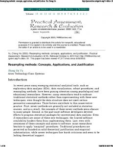
mean F1 value
06 :
PDDP SPC ARG AIB DSR WSR FIG. 2. Direct comparison of the clustering methods. The bars indicate mean and standard deviation of the mean F1 -values obtained by applying the different methods to the 800 documents experiments in the first (upper bars) and second (lower bars) database.
As mentioned above we here put aside the interesting question of how to find the good clusters within the tree, i.e. estimate in an unsupervised way which clusters at which resolution are good approximations of the underlying categories. Thus the values presented in tables III and IV are upper bounds for what is achievable with any such search algorithm. We think that this problem can be separated from the basic clustering problem as the occurrence of good clusters in the tree is of course the prerequisite that limits all achievements of any algorithm that searches the tree for good clusters.
0:6 0:4 0:2
0
1
2
3
4
1
mean F1 value
:
:
0:8
5
6
log2 NR
7
8 ARG DSR AIB SPC WSR
0:8 0:6
96 ± 9 136 ± 32 286 ± 54 801 ± 50 9678 ± 1192
TABLE V. Computational cost in seconds. All values correspond to applying the algorithms to the 800 experiment of the first database. The CPU has been PIII with 650 MHz. PDDP was run under MATLAB and thus cannot be compared.
0:4 0:2 0
07
05
1
0
08
0
1
2
3
4
5
6
log2 NR
7
8 V. CONCLUSIONS
FIG. 1. Dependence of the clustering performance of the resampling methods WSR (applied to the 200 experiment, upper graph) and DSR (applied to the 800 experiment, lower graph) on the number of subsamples. Saturation occurs at 64 subsamples for the WSR method. DSR works best at NR = 32. The solid line corresponds to the first database, the dashed line to the second.
We find that the quality of the clustering results depends to a large extent on the dataset. In particular we observe that the performance as measured in this paper is almost always better on larger categories. When comparing the results of single categories in the 800 and 8
EQ experiments, we find that they are better in the case where the number of documents of that category is larger. For example in the second database categories “trade”, “crude”, “grain”, “money-fx” are larger in the 800 experiment and the results are also better in the 800 experiment. All other categories are larger in the EQ experiment and also there are the better results for these categories. Also in this way the categories “ship” and “money-supply” can be better resolved in the context of the first database.
ACKNOWLEDGMENTS
We are grateful to E. Domany, G. Getz, S. Gnutzmann and A. Shehter for useful discussions. This work was partially supported by the Minerva foundation.
Also we think that the resolvability of a category is influenced by interference with other categories in the dataset through an overlap of the characteristic word fields. We believe that if the characteristic words of a category are also used in documents of other categories that category can not be resolved as good as if there were no close categories.
[1] J.A. Hartigan, Clustering algorithms (John Wiley & Sons, New York, 1975). [2] A.K. Jain and R.C. Dubes, Algorithms for clustering data (Prentice-Hall, Englewood Cliffs, New Jersy, 1988). [3] D. Boley, M. Gini, R. Gross, E.H. Han, K. Hastings, G. Karypis, V. Kumar, B. Mobasher, and J. Moore, Document categorization and query generation on the World Wide Web using WebACE, Artif. Intell. Rev. 13 (5-6) 365-391 (1999). [4] M. Blatt, S. Wiseman, and E. Domany, Superparamagnetic clustering of data, Phys. Rev. Lett. 76 (18) 32513254 (1996). [5] M. Blatt, S. Wiseman, and E. Domany, Data clustering using a model granular magnet, Neural Comput. 9 (8) 1805-1842 (1997). [6] A. Strehl, J. Ghosh, and R. Mooney, Impact of similarity measures on web-page clustering, in Proc. of the 17th National Conference on Artificial Intelligence: Workshop of Artificial Intelligence for Web Search, p. 58-64 (AAAI, 2000). [7] G. Getz, E. Levine, and E. Domany, Coupled two-way clustering of gene microarray data, Proc. Nat. Acad. Sci. USA 97 (22) 12079-12084 (2000) [physics/9911038]. [8] E.Levine and E.Domany, Unsupervised estimation of cluster validity using resampling, Neural Comput. (in print). [9] http://www.research.att.com/~lewis/reuters21578.html [10] D. Fisher, Critical behavior of random transverse-field Ising spin chains, Phys. Rev. B 51 (10) 6411-6461 (1995). [11] N. Slonim and N. Tishby, Agglomerative information bottleneck, in Advances in Neural Information Processing Systems 12, edited by S.A. Solla, T.K. Leen, and K.-R. M¨ uller (MIT Press, 1999). [12] N. Tishby, F. Pereira, and W. Bialek, The information bottleneck method, in 37th Annual Allerton Conference on Communication, Control, and Computing, p.368-377 (1999). [13] R. O. Duda and P. E. Hart, Pattern classification and scene analysis (John Wiley & Sons, New York, 1973). [14] D. Boley, Principal direction divisive partitioning, Data Min. Knowl. Disc. 2 (4) 325-344 (1998). [15] C.J. van Rijsbergen, Information retrieval (Butterworths, London, 1979). [16] A.N. Strugatsky, B.N. Strugatsky, Otel’ “U pogibshego alpinista”, Yunost’ 9-11 (1970) [Inspector Glebsky’s Puzzle (Richardson & Steirman & Black, New York, 1988)].
Comparing the results for the “money-supply”, “ship” and “sugar” categories in the EQ experiments of the two databases gives a clue to possible interference. We find that “money-supply” and “ship” are better resolved in the EQ experiments on the first database, whereas “sugar” is better in the second database. Further we observe that some categories appear to have a preferred algorithm or vice versa. So SPC performance in the EQ experiment of the second database peaks in categories “trade”, “money-supply” and “interest” whereas the results for the other categories are only moderate. However, the ranking of the performance of different clustering methods does not sensitively depend on the data. We found that the level of performance of SPC, ARG and AIB is almost the same. Results obtained with PDDP are not as good, whereas the advantage of this method is that it is much faster on large databases. PDDP does not require the calculation of a (dis-)similarity matrix and its time consumption scales linear with the number of documents. The feature selecting methods that we propose in this paper can improve the results. WSR yields the highest performance but has on the other hand a very high computational cost. As it is implemented, the required time scales with n3 . DSR gives moderate improvement of the clustering quality but is in comparison to WSR much faster. The time consumption of DSR is dominated by the size of the subsets. Thus for large datasets, if one can probe the discriminative words with comparably small subsets it will be faster than SPC, AIB and ARG that all rely on the computation of a complete distance matrix on the basis of the whole word set. Another little advantage of the feature selecting methods is that the application of a stoplist becomes obsolete, WSR and DSR perform as good on the raw data matrix.
9