COMPARISON OF STANDARD RESAMPLING METHODS FOR ...

COMPARISON OF STANDARD RESAMPLING METHODS FOR PERFORMANCE ESTIMATION OF ARTIFICIAL NEURAL NETWORK ENSEMBLES Michael Green1 and Mattias Ohlsson1 1

Computational Biology and Biological Physics Group, Department of Theoretical Physics, Lund University, Sweden [email protected]

Keywords: artificial neural networks, performance estimation, k-fold cross validation, bootstrap

Furthermore, when using ANN ensembles it is important to incorporate all model training and model selection procedures within the performance estimation loop to avoid information leakage that would otherwise bias the estimation. The aim of this study was to compare five common resampling methods for estimating the generalization performance of an ANN ensemble on five datasets. All of them were binary classification problems. First we tried to numerically establish which of the resampling methods that came closest to the true performance. Second we investigated whether the choice of resampling method for model selection had any influence on the true performance as estimated by the outer resampling method. Two common ensemble creation techniques were used, bagging [3] and the cross validation ensemble [6].

INTRODUCTION

METHODS

Machine learning applications for classification in medicine is developing rapidly today and the question of how to best evaluate them has been addressed by many scientists. In the machine learning community it is well known that when training a classifier one should set aside a portion of the data for testing. Preferably this procedure should be repeated a number of times to collect statistics. Methods such as K-fold cross validation (CV), bootstrap [4] and holdout methods have been developed for dividing data into a training and test set. Rigorous resampling procedures are especially important when dealing with unstable learners such as Artificial Neural Networks (ANN) [1]. This machine learning concept has been used extensively over the years in many different areas of pattern recognition. It is common knowledge that CV gives a nearly unbiased estimate of the performance of a classifier. However, this only applies if all aspects of model training is carried out within the CV loop [14]. Also CV often pay for this low bias in terms of large variance. In the late 90’s Efron et. al. [4] introduced the .632+ bootstrap method as an improvement over CV. This method maintained low variance. There are, however, also reports that the .632+ rule can give large bias. Molinaro et. al. [10] found the .632+ method to be severely biased when dealing with high dimensional genomic data, and that CV, despite its large variance, was better at estimating the true performance of a classifier. Few comparisons of standard resampling methods for performance estimation has been conducted as of today [10, 8] and there is currently, to our knowledge, no study focusing on ANN ensembles.

Datasets

Abstract: Estimation of the generalization performance for classification within the medical applications domain is always an important task. In this study we focus on artificial neural network ensembles as the machine learning technique. We present a numerical comparison between five common resampling techniques: k-fold cross validation (CV), holdout, using three cutoffs, and bootstrap using five different data sets. The results show that CV together with holdout 0.25 and 0.50 are the best resampling strategies for estimating the true performance of ANN ensembles. The bootstrap, using the .632+ rule, is too optimistic, while the holdout 0.75 underestimates the true performance.

Five datasets were used in this study. Three real world and two simulated datasets. The first real world dataset contained 12-lead electrocardiogram (ECG) data extracted from chest pain patients suspected of having transmural infarction (TMI) [11]. We used 18 features from the ECG and the training and test set consisted of 1000 and 3000 data points respectively. The second real world dataset was the Wisconsin Breast Cancer Database [9]. This breast cancer database was obtained from the University of Wisconsin Hospitals, Madison from Dr. William H. Wolberg. The database contained 699 patients of which 458 was diagnosed benign and 241 as malignant. In total 10 features was collected from each patient. Real world dataset number three was collected in 1997 and comes from 862 consecutive patients attending the Lund University emergency department with a principal complaint of chest pain [5, 2]. The diagnosis was either Acute Coronary Syndrome (ACS) or non-ACS. We used 16 PCA components extracted from 12-lead ECG recordings. Simulated dataset 1 contained data drawn from two multivariate Gaussian distributions with equal mean but with different covariance matrices. Specifically the two classes were generated from p(x|Ck ) = N (x|µ, σk2 I) where I is the identity matrix, and σk2 the variance for class Ck . The input vector x is eight dimensional and the size of the training and test set was 600 and 10000 respectively.

The second simulated dataset was acquired from two overlapping multivariate Gaussian distributions with equal covariance matrices but differing mean, as p(x|Ck ) = N (x|µk , σ 2 I) where I is the identity matrix, and µk the mean vector for class Ck . The number of dimensions and the number of samples in the training and test set was the same as the first simulated dataset. Artificial neural networks ensembles We used ANN in the context of bagging [3] or CV ensembles [6] of size 25 and 24, respectively, which has been found to be sufficient in numerical studies [12]. The individual ensemble member ANNs were implemented as fully connected feedforward multilayer perceptrons (MLP) with no direct input-output connections. Only one hidden layer with five hidden units was used for all datasets. Each individual ANN in the ensemble was trained using a Quasi-Newton algorithm with the kullback-leibler error function for two classes X E= (tn ln yn + (1 − tn ) ln(1 − yn )) + αEreg n

featuring a weight-elimination term Ereg =

X i

ω02

ωi2 + ωi2

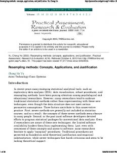
to possibly regularize the network. The sum runs over all the weights in the network except the biases. The reason for excluding the biases from the penalty term is that we do not wish to force the decision boundary to pass through the origin in input space. The CV ensemble method was used as follows: The training set was randomly divided into two parts of equal size. Two ensemble members were created by training one MLP on each of the two parts. This procedure was repeated 12 times, with a new random division each time. The resulting CV ensemble consisted of 24 MLPs. Performance estimation We used the area under the receiver operating characteristic curve (AUC) as a performance measure for a given ANN ensemble. The AUC can be interpreted as the probability that a randomly chosen data point from class C1 has a higher output value than a randomly chosen data point from class C2 [7]. The choice of AUC as the performance measure was mostly governed by its popularity, but also because it is independent of any cut on the output value. In every dataset used in this study we put aside a large fraction (approximately 70%) to be used as an independent test set. The remaining data was used to estimate the performance of the ANN ensemble using five different resampling methods. The true performance of the ANN

Fig. 1: Illustration of the performance estimation procedure. The data set is split into an independent test set and a training set. The latter is further divided into a TstP and a TrnP set used for the performance evaluation. The TrnP is finally split into a ValM and a TrnM set for the model selection. The methods used to split the data sets are indicated in the balloons. ensemble was evaluated by training an optimal ANN ensemble on the remaining data and testing on many bootstrap samples of the test set. The optimal model was chosen by a model selection procedure described later. In other words we used the performance of the ANN ensemble on the test set as a baseline for comparing the capability of the different resampling methods for correctly estimating the true performance. The whole procedure is illustrated in Figure 1. Five resampling methods was investigated; 5x5 fold CV, 25 fold bootstrap and 25 fold holdout using three cutoffs (0.25, 0.50 and 0.75). Thus, each method produced 25 new test and training data sets, labeled TstP and TrnP in Figure 1, from the original training data. We built an optimized ANN ensemble for every training set (TrnP) using a model selection procedure described in the next section. The best model was then tested on the corresponding test data (TstP). This resulted in 25 training and test results that we used to estimate the performance of the ANN ensemble for each method. We used the mean of the 25 test AUCs for the CV and the holdout techniques, meanwhile the .632+ rule was used when evaluating the bootstrap method. This rule is less biased than its predecessor since it corrects, to some extent, for overfitting. Model selection The model selection consisted of a grid search for the optimal weight elimination parameter α. For each value of α an inner resampling session using bootstrap or CV was carried out on the training data. This process is also illustrated in Figure 1. We used 25 resamples for the inner loop, i.e., a 5x5 fold CV or a 25 fold bootstrap. A full

ANN ensemble was built from each resample (TrnM) using bagging [3] or the CV ensemble [6]. The α receiving the best AUC from the inner loop was used to construct an ANN bagging ensemble on the whole training set (TrnP).

CV Bootstrap HO 0.25 HO 0.50 HO 0.75 True

Optimal Bayes classifier for simulated data The two artificial datasets were generated from variants of the multivariate Gaussian distribution. Knowing the generating distribution allows us to derive the optimal Bayes classifier, that is, we can evaluate the posterior probability for class C1 given the data using Bayes’ theorem. Following Bishop [1] and taking the functional form of the posterior to be sigmoid we set p(C1 |x) =


1 p(x|C1 )p(C1 ) = p(x|C1 )p(C1 ) + p(x|C2 )p(C2 ) 1 + e−a


so that a = ln

p(x|C1 )p(C1 ) p(x|C1 ) = ln p(x|C2 )p(C2 ) p(x|C2 )

using the fact that we have p(C1 ) = p(C2 ). Setting a = 0 gives us the decision boundary for our problem, corresponding to a cut of 0.5. For simulated data 1 this can be interpreted as a hypersphere with radius r2 =

2 σ2 · ln . 1/σ12 − 1/σ22 σ1

Training Validation Simulation 1 0.97 0.87 0.99 0.94 0.97 0.86 0.99 0.85 1.00 0.79 0.96 0.88 Simulation 2 0.97 0.87 0.99 0.94 0.98 0.86 0.99 0.84 1.00 0.79 0.88 0.86 ACS 0.91 0.76 1.00 0.90 0.93 0.76 0.96 0.75 0.99 0.71 0.86 0.77

Test 0.86 0.89 0.86 0.85 0.80 0.88 0.87 0.90 0.86 0.86 0.80 0.84 0.73 0.79 0.75 0.73 0.70 0.76

Table 1: Results for all five resampling methods on ACS and both simulated datasets using bagging ensembles and CV for the model selection. The results are presented as mean AUC, except for the bootstrap method where the .632+ estimator was used.

The corresponding interpretation for simulated data 2 is a hyperplane defined by µ ¶T µ1 − µ2 µ2 − µ2 x + 2 2 1 = 0. 2 σ 2σ 0.9

0.8

0.7

HO 0.75

HO 0.75

HO 0.75

HO 0.50

HO 0.25

HO 0.25

HO 0.25

Bootstrap

Bootstrap

Bootstrap

CV

CV

CV

True

True

The results for the five data sets using bagging ensembles and CV in the model selection are presented in Table 1 and 2. The CV and holdout using cuts 0.25 and 0.50 had similar performance for all datasets. They differed with at most three percent from each other. See Figure 3 and 2. These three methods also did a good job estimating the true performance with differences ranging from one to three percent. The holdout 0.75 and bootstrap methods were strongly biased for the majority of the datasets, and rarely performed well. The bootstrap constantly overestimated the true performance meanwhile the holdout 0.75 remained rather pessimistic in its estimation. The true validation result was defined as the largest AUC during the model selection procedure on the whole training set. A closer look at the validation results revealed a bias for the holdout 0.75 method. It underestimated the validation performance with 4 to 12 percent.

True

RESULTS

HO 0.50

Simulated 1 Simulated 2 ACS

0.6

HO 0.50

Test AUC

The performance of these classifiers was estimated, using AUC, by evaluating them on one hundred thousand samples from each class. Their performance should serve as an upper bound for the ANN ensemble since the ANN is known to estimate the Bayesian posterior probability [13].

Fig. 2: Boxplots for ACS data and for Simulated data 1 and 2 using bagging ensembles and CV for the model selection. The opposite was true for the bootstrap method. It overshot the true validation performance by magnitudes ranging from 1 to 14 percent. The CV, holdout 0.50 and 0.25 methods only differed slightly from the true validation performance. Turning our eyes to the CV ensembles in Table 3 and 4 we see that the results closely resembles the results for the bagging ensembles. Comparing the box plots in Figure 5 and 4 with Figure 3 and 2, no obvious differences could be found between CV and bagging ensembles for any of

Training Validation Breast cancer 1.00 0.99 1.00 1.00 1.00 0.99 1.00 1.00 1.00 0.87 1.00 0.99 TMI 0.99 0.94 1.00 0.97 0.99 0.92 0.99 0.91 0.99 0.87 0.99 0.94

CV Bootstrap HO 0.25 HO 0.50 HO 0.75 True CV Bootstrap HO 0.25 HO 0.50 HO 0.75 True

Test 0.99 0.99 0.99 0.99 0.99 0.99


0.93 0.95 0.94 0.92 0.88 0.93


Table 2: Results for all five resampling methods on Breast cancer and TMI data using bagging ensembles and CV for the model selection. The results are presented as mean AUC, except for the bootstrap method where the .632+ estimator was used.

Test 0.87 0.90 0.87 0.85 0.80 0.88 0.87 0.90 0.87 0.85 0.80 0.83 0.72 0.79 0.75 0.73 0.70 0.76

Table 3: Results for all five resampling methods on ACS and both simulated datasets using CV ensembles and CV for the model selection. The results are presented as mean AUC, except for the bootstrap method where the .632+ estimator was used.

1.00

0.95

0.90

DISCUSSION AND CONCLUSION

0.85

HO 0.75

HO 0.75

HO 0.50

HO 0.50

HO 0.25

Bootstrap

Bootstrap

CV

CV

True

True

Breast Cancer TMI HO 0.25

Test AUC


Training Validation Simulation 1 0.97 0.87 0.99 0.94 0.97 0.87 0.98 0.84 0.99 0.78 0.95 0.88 Simulation 2 0.97 0.87 0.99 0.94 0.98 0.87 0.99 0.84 0.99 0.79 0.88 0.86 ACS 0.92 0.76 0.99 0.90 0.94 0.76 0.97 0.76 0.99 0.72 0.92 0.76

Fig. 3: Boxplots for the Breast cancer data and the TMI data using bagging ensembles and CV for the model selection. the data sets. Training a single MLP instead of an entire ensemble resulted in a downward bias for all datasets. All methods underestimated the true performance to a larger extent than when using ensembles indicating that the single MLP was not able to generalize as well from the data. Boxplots for the single MLP are shown in Figures 6 and 7. Using the .632+ bootstrap estimator during the model selection produced the same estimation of the true performance as the CV. However, the models selected by the two different strategies differed as well as the corresponding AUCs. Looking closer into the values of the regularization parameter α selected by the two different model selection methods we found that most α’s were small, indicating that no or very little regularization were optimal for the ensembles.

In this paper we examine five common resampling methods for the purpose of estimating the generalization performance using ANN classification ensembles. The process of training an ANN ensemble also includes resampling methods for creating the ensemble and resampling methods for the model selection part. To limit the number of combinations of resampling methods to test, the ensemble creation was limited to the bagging and cross validation ensemble. Furthermore, in the model selection part only two resampling methods were tested, CV and bootstrap. Although CV and bootstrap gave different estimations of the true test performance, no difference was found when using them in the model selection part. The reason for this is probably because the purpose of the model selection is to determine the regularization parameter α. Now for ANN ensembles in general one expects little or no regularization at all, and this was confirmed in our results since the selected models had overall small α’s. The model selection part is therefore not crucial, hence no difference between CV and bootstrap. In this study no feature selection was performed since the input variables were predefined. When including feature selection in the model selection process it may turn out that different resampling methods for the model selection will give different results. Turning to the true performance estimation results we found that CV, holdout 0.25 and 0.50 performed

1.00

0.95

0.85

Table 4: Results for all five resampling methods on Breast cancer and TMI data using CV ensembles and CV for the model selection. The results are presented as mean AUC, except for the bootstrap method where the .632+ estimator was used.

HO 0.75

HO 0.75

HO 0.50

HO 0.25

HO 0.25

Bootstrap

Bootstrap

CV

CV

Breast Cancer TMI HO 0.50

0.93 0.95 0.92 0.92 0.87 0.92

0.90

True


0.99 0.99 0.99 0.99 0.99 0.99

Test AUC


Test

True

Training Validation Breast cancer 1.00 0.99 1.00 1.00 1.00 0.99 1.00 1.00 1.00 0.95 1.00 0.99 TMI 0.99 0.92 1.00 0.97 0.99 0.92 0.99 0.91 0.98 0.87 0.98 0.94

Fig. 5: Boxplots for the Breast cancer data and the TMI data using CV ensembles and CV for the model selection.


Test AUC

0.9

0.8

0.7

0.9

HO 0.75

HO 0.75

HO 0.75

HO 0.75

HO 0.50

HO 0.50

HO 0.50

HO 0.25

HO 0.25

HO 0.25

Bootstrap

Bootstrap

Bootstrap

CV

CV

CV

True

Fig. 6: Boxplots for ACS data and for Simulated data 1 and 2 using a single MLP and CV for the model selection. HO 0.75

HO 0.75

HO 0.50

HO 0.25

HO 0.25

HO 0.25

Bootstrap

Bootstrap

CV

Bootstrap

CV

CV

True

True

True

HO 0.50


0.6

True

True 0.7

HO 0.50

Test AUC

0.6 0.8

Fig. 4: Boxplots for ACS data and for Simulated data 1 and 2 using CV ensembles and CV for the model selection. equally well. The bootstrap method, using the .632+ rule, was constantly overestimating the test performance. Although the .632+ rule should compensate for possible overfitting, which is the case for the individual members of the ensemble, it is still biased. The holdout 0.75 resampling method was on the other hand constantly underestimating the true performance. This is probably due to the low fraction of data used to construct the ANN ensemble, hence a very inaccurate model. Lingering on the true performance we found that the ANN ensemble succeeded to reach the optimal Bayes estimate using the second artificial data set. The first artificial problem was much more difficult and the true performance of the ANN ensemble did not match the Bayes estimate of 0.93. However, this was mainly an effect of undersampling since only 600 data points were used to construct the ANN ensemble. Increasing the flexibility of

the networks as well as the amount of data available to the construction of the ANN ensemble alleviated this problem, indicating that our definition of truth made sense. In this study we tested five different data sets, originating from three medical classification problems and two artificial ones. The medical applications ranged from being difficult to very easy. For the simulated data sets, one was linear and the second one required nonlinearity for the optimal solution. The advantage of using simulated data is of course the unlimited amount of test data. Although only a small number of data sets were used we believe that they represents suitable mix of different classification problems. In conclusion we found, for our choice of data sets and training procedures, the best resampling strategies for estimating the true performance of an ANN ensemble to be the CV and holdout, using cutoff 0.25 and 0.50, methods. The .632+ bootstrap did not match this performance but still gave a much more accurate estimation than holdout 0.75. The choice of resampling technique in the model selection did not influence the final estimation. We can also confirm the well known advantage of using ANN ensembles compared to single ANNs.

[7] J. A. Hanley and B. J. McNeil. The meaning and use of the area under a receiver operating characteristic (roc) curve. Radiology, 143(1):29–36, Apr 1982.

1.00

[8] R. Kohavi. A study of cross-validation and bootstrap for accuracy estimation and model selection. In Proceedings of the Fourteenth International Joint Conference on Artificial Intelligence, pages 1137– 1145. Morgan Kaufmann, 1995.

Test AUC

0.95

0.90

0.85

0.80

HO 0.75

HO 0.75

HO 0.50

HO 0.25

HO 0.25

Bootstrap

Bootstrap

CV

CV

True

True

HO 0.50

Breast Cancer TMI

0.75

Fig. 7: Boxplots for the Breast cancer data and the TMI data using a single MLP and CV for the model selection. ACKNOWLEDGMENTS This work has been supported by the Swedish Knowledge Foundation through the Industrial PhD program in Medical Bioinformatics at the Strategy and Development Office (SDO) at the Karolinska Institute. REFERENCES [1] C. M. Bishop. Neural Networks for Pattern Recognition. Oxford University Press, 1995. [2] J. Björk, J. L. Forberg, M. Ohlsson, L. Edenbrandt, H. Ohlin, and U. Ekelund. A simple statistical model for prediction of acute coronary syndrome in chest pain patients in the emergency department. BMC Medical Informatics and Decision Making, 6:28, 2006. [3] L. Breiman. Bagging Predictors. Machine Learning, 24:123–140, 1996. [4] B. Efron and R. Tibshirani. Improvements on crossvalidation: The .632+ bootstrap method. Journal of the American Statistical Association, 92(438):548– 560, June 1997. [5] M. Green, J. Björk, J. Forberg, U. Ekelund, L. Edenbrandt, and M. Ohlsson. Comparison between neural networks and multiple logistic regression to predict acute coronary syndrome in the emergency room. Artificial Intelligence in Medicine, 38(3):305–318, Nov 2006. [6] M. Green, J. Björk, J. Hansen, U. Ekelund, L. Edenbrandt, and M. Ohlsson. Detection of acute coronary syndromes in chest pain patients using neural network ensembles. In J. M. Fonseca, editor, Proceedings of Computational Intelligence in Medicine and Healthcare, pages 182–187, Lisbon, Portugal, June-July 2005. IEE/IEEE.

[9] O. L. Mangasarian and W. H. Wolberg. Cancer diagnosis via linear programming. SIAM News, 23(5):1,18, 1990. [10] A. M. Molinaro, R. Simon, and R. M. Pfeiffer. Prediction error estimation: a comparison of resampling methods. Bioinformatics, 21(15):3301–3307, Aug 2005. [11] S.-E. Olsson, M. Ohlsson, H. Ohlin, S. Dzaferagic, M.-L. Nilsson, P. Sandkull, and L. Edenbrandt. Decision support for the initial triage of patients with acute coronary syndromes. Clinical Physiology and Functional Imaging, 26(3):151–156, May 2006. [12] D. Opitz and R. Maclin. Popular ensemble methods: An empirical study. Journal of Artificial Intelligence Research, 11:169–198, 1999. [13] M. D. Richard and R. P. Lippmann. Neural network classifiers estimate bayesian a posteriori probabilities. Neural Computation, 3:461–483, 1991. [14] S. Varma and R. Simon. Bias in error estimation when using cross-validation for model selection. BMC Bioinformatics, 7:91, 2006.