Research Article Constrained Quadratic Programming
Recommend Documents
May 1, 1997 - Kaj Madsen · Hans Bruun Nielsen · Mustafa Ã. Pınar ... K. Madsen, H.B. Nielsen: Institute of Mathematical Modelling, Technical University of ...
Abstract. In this contribution we consider the problem of regression estimation. .... Besides the tensor product formalism of ANOVA models, which we present in.
communications, an ever-increasing demand of substantially higher throughput is a ... the pilot reuse is inevitable in massive MIMO systems, and the imperfect ...
Mar 4, 2014 - Kiehl and Jerzak [22] studied a gun tube damped by a constrained viscoelastic polymer. The system was analysed through a time domain ...
a set of linear equalities and complementarity constraints. Much like in separable programming, a modified version of th
Dec 15, 2010 - Volume 2009, Article ID 257197, 9 pages doi:10.1155/2009/ ..... The PSD of the microphone signal Xk ...... Webpage:ȱwww.eusipco2011.org.
[13] O. Juan and R. Keriven, âTrimap segmentation for fast and user-friendly alpha matting,â in VLSM, LNCS 3752, 2005, pp. 186â197. [14] V. Kolmogorov, A.
Jia Xu,1,2,3 Chuan Ping Wang,1 Hua Dai,1,2 Da Qiang Zhang,4 and Jing Jie Yu3 ... Correspondence should be addressed to Jia Xu; [email protected].
1579â1588, 2007. [12] G. Venter and J. Sobieszczanski-Sobieski, âParticle swarm opti- .... Intelligence, John Wiley & Sons, New York, NY, USA, 2005. [54] I. C. ...
Nov 20, 2013 - phone or Skype) to clarify and correct the answers where needed. In addition, the .... Perth lets the patients chose between FS4 and FS4p and.
may also be combined with various programming order techniques that mitigate the ..... http://newsroom.intel.com/community/intel_newsroom/blog/2011/04/14/.
Ali Pezeshki, Louis L. Scharf, Magnus Lundberg, and Edwin K. P. Chong ... Engineering, and Mathematics, Colorado State University, Fort Collins, CO. 80523 ...
Sep 16, 2015 - (defined as the set of solutions that can be obtained by flipping a single ..... IEEE Symposium on Foundations of Computer Science (Las Vegas, ...
2015, Modares and Lewis, 2014, Song and Yan, 2014, Alt and. Seydenschwanz, 2014) .... varied in time according to some criterium, e.g. energetic or economic costs. 3. ..... International Journal of Robust and Nonlinear Control,. 9:1117–1141 ...
Marcelo S. Reis1. 1 Center of Toxins, Immune-response and Cell Signaling (CeTICS);. Laboratório Especial de Ciclo Celular, Instituto Butantan, SËao Paulo, ...
Jun 14, 2006 - e-mail: [email protected]. R. Shioda ( ). Department of Combinatorics and Optimization, Faculty of Mathematics, University of Waterloo,.
A nice feature of this function is that it is continuously differentiable. This makes it
... study of control systems with saturating actuators and state constraints.
Jun 14, 2006 - Algorithm for cardinality-constrained quadratic optimization. Authors of [2, 9, 10] use pivoting and enumeration to search for subsets with.
2A linear system is said to be semi-stable if all its poles are in the closed left-half plane. variant set .... V(x) - 2xTP(Ax + Bsat(Fx)) < 0. (5) for all x e $(P, p) \ {0}.
May 9, 2007 - Sequential (or Successive) Quadratic Programming (SQP) is a ...... automatic differentiation within modelling languages such as AMPL, GAMS ...
the solution of bound and/or equality constrained quadratic programming prob- lems. The unique ..... BE = {x ∈ IRnt : Ctx = o and x ≥ lt}, qt(x) = 1. 2. xTAtx − bT.
for General Stochastic Bottleneck Spanning Tree Problems. Jue Wang ... The problem minimizes a scalar and seeks a spanning tree, of which the maximum.
using relational databases within the Esterel programming language. We choose MySQL [10] as the database and, since reactive kernels are produced as C ...
Dynamic Programming-Based Energy Management System for. Range-Extended Electric Bus. Xiaogang Wu, Jingfu Chen, and Chen Hu. College of Electrical ...
Research Article Constrained Quadratic Programming
Sep 17, 2017 - 1, pp. 15â25, 2017. [5] A. Amanatiadis, âA Multisensor Indoor Localization System for Biped Robots Operating in Industrial Environments,â IEEE.
Hindawi Mathematical Problems in Engineering Volume 2017, Article ID 6725427, 15 pages https://doi.org/10.1155/2017/6725427
Research Article Constrained Quadratic Programming and Neurodynamics-Based Solver for Energy Optimization of Biped Walking Robots Liyang Wang,1 Ming Chen,1 Xiangkui Jiang,2 and Wei Wang3 1
Department of Electronic Engineering, Shunde Polytechnic, Foshan, Guangdong 528300, China School of Automation, Xi’an University of Posts and Telecommunications, Xi’an 710121, China 3 College of Power and Mechanical Engineering, Wuhan University, Wuhan 430072, China 2
1. Introduction Biped robots receive a lot of attention from the scientists and engineers these years [1–10]. Compared with wheeled driven robots and crawler robots, biped robots have anthropomorphic adaptability to unstructured environments with relative less energy consumption. However, Honda’s ASIMO, perhaps representative of humanoid robots, uses at least 10 times the energy (scaled as dimensionless specific cost of transport) of a typical human [11]. Energy consumption of the existing biped robots is much more than that of human being. Two main kinds of approaches have been presented to optimize the energy efficiency for legged robots: the first type focuses on the improvements of mechanical device [11– 14] and the second type is devoted to better optimization algorithm [15–19]. A well-known improvement of biped mechanical device is brought by “semipassive walkers.” Numerous very successful “semipassive walkers” have been built [11], such as the Cornell biped, the Delft biped, and the MIT learning biped robots. These robots are built based on passive dynamics, with
small active power sources substituted for gravity, which can walk on level ground. However, uneven ground leads to falls of the Cornell biped robot and floor irregularities lead to falls of the Delft biped robot. Although the MIT learning biped robot continually learns and adapts to the terrain as it walks, its energy consumption is especially high. From another aspect, several auxiliary devices are designed to decrease energy consumption of legged robots. In [12], an elastic load suspension mechanism was developed and utilized on a hexapod robot to increase the energy efficiency of legged robot locomotion. The experiments demonstrate that the robot with an elastically suspended load consumed up to 24% less power than with a rigidly attached load. In [13], a flexible shoe system was proposed for biped robots to optimize energy consumption of the lateral plane motion. The shoe system can absorb the kinetic energy of the robot, which is confirmed by simulations and experiments. In [14], the energy efficiency of a humanoid robot with spinal motion was investigated. Simulations show that, with the additional degrees of freedom (DoF) in the torso, the robot
2 requires 26.5% less energy than its rigid-torso counterpart to complete the same walking. Differing from various mechanical devices for decreasing the energy consumption of legged robots, optimization algorithms can be used more widely because this kind of approach is applicable to all the robots with actuators. Motivated by trunk rotations of human being, an algorithm based on fuzzy logic and iterative optimization [15] provides a remarkable descend rate of energy consumption for biped robots. In [16], an online gait synthesis algorithm compromising waking stability and energy efficiency is proposed and the parameters are optimized for a given travel distance minimizing the energy consumed by the actuators. In [17], a reference generation algorithm was proposed for biped robots based on linear inverted pendulum model. Simulation results suggest that the proposed moving zero-moment-point (ZMP) references are more energy-efficient than the ones with fixed ZMP under the supporting foot. However, when decreasing the energy consumption of biped robots, the reported works neglect the inevitable presence of some inside constraints, including the reaction forces from the ground, frictional force between the feet and the ground, and some limitations of the biped joints. On the other hand, some recent works have been done in modeling, measuring, estimating, and rejecting the undesired force introduced to the dynamics of robots. Fakoorian et al. [18] designed a continuous-time extended Kalman filter (EKF) and a continuous-time unscented Kalman filter (UKF) to estimate not only the states of the robot system but also the ground reaction forces that act on the foot. Moosavi et al. [19] designed a nonlinear controller for second-order nonlinear uncertain dynamical systems. The results demonstrate that the proposed method is a partly model-free controller that works well in certain and partly uncertain system. Differing from the existing literatures, the proposed neurodynamicsbased energy optimization (NEO) strategy minimizes the energy consumption and guarantees the following three important constraints simultaneously: (i) the force-moment equilibrium equation of biped robots, (ii) frictions applied by each leg on the ground to hold the biped robot without slippage and tipping over, and (iii) Physical limits of the motors. In this work, in order to provide optimal controller to meet all the above-mentioned constraints, a QP problem is formulated to deal with the constrained optimization problem. Utilizing the dynamics model, an objective function based on energy-efficiency optimization can be computed so that the control input can be produced within system constraints. Furthermore, the optimized control outputs need to be available as the robot moves on at each step. Therefore, online implementation is the next fundamental issue in the energy efficiency optimization. Whether the energy optimum control can be implemented successfully is dependent on the efficiency of online optimization. To solve the proposed constrained optimization problem in real time, neurodynamics-based QP solvers are considered because of their sufficient online computational power [20– 22]. Several optimal controls for robots have been realized using neural network optimization [23–25]. In this paper, considering the physical constraints on biped motions, a
Mathematical Problems in Engineering novel neurodynamics-based energy-efficiency optimization controller is developed. The strategy for optimizing the energy efficiency is formulated as a constrained QP problem, which can be solved online using a primal-dual neural network (PDNN). Simulation studies are presented to illustrate the feasibility of the proposed strategy. Main contributions of this work could be summarized as follows: (i) A new complete model for energy optimization of biped walking robots is built. Several necessary physical constraints for the biped system are formulated in the optimization controller, which provides a more practical objective for the energy optimization of biped robots. (ii) A neurodynamics-based solver is presented to handle the proposed optimization problem. To the best of our knowledge, no works on biped walking using energy optimum control based on neural network have been reported before. The organization of this paper is as follows. In Section 2, the background about the energy consumption of biped walking robots is presented. A QP problem for the energy optimization is formulated in Section 3. Section 4 proposed a neurodynamics-based solution for the proposed QP problem to realize the energy optimization. Section 5 presented the diagram of the neurodynamics-based energy optimization control system. Simulation results are provided in Section 6, followed by the conclusions in Section 7.
2. Energy Consumption of a Biped Walking Robot The main idea is to optimize the energy consumption of a biped robot walking on horizontal ground. For optimization purposes, we consider the following assumptions. Assumption 1. We assume that the robot walks on practicable horizontal terrain. Therefore, there are no forbidden zones, and every foot can be placed on the ground and provide support to the robot. Assumption 2. We assume that all the motors in the biped joints have the same configurations. The robot’s actuators are based on DC electric motors (electrical motors cannot store the gains of negative energy) [26, 27]. Assumption 3. Consider a biped robot with point contacts between the ground and each foot. Assume that each foot contacts the ground with Coulomb friction. The energy consumption of a biped robot is given by the sum of the energy consumed in every joint plus the energy consumed by electronic equipment (computers, drivers, analog I/O, etc.). The contribution of the latter is out of the scope of this work.
Mathematical Problems in Engineering
3
If a joint is driven by an electrical motor, the consumed energy is given by 𝐸 (𝑡) = ∫ 𝑢 (𝑡) 𝑖 (𝑡) 𝑑𝑡,
where 𝑖 = 1, 2 denotes the serial number of the legs and 𝑗 = 1, . . . , 𝑛 is the serial number of the joints/motors in one leg. The function Δ(⋅) is defined as
(1) {𝑦 if 𝑦 > 0; Δ (𝑦) = { 0 if 𝑦 ≤ 0. {
where 𝑢(𝑡) is the voltage and 𝑖(𝑡) is the current through the motor. As a normal practice in modeling DC motors for robotic joints [27], the following electrical model of a motor is considered here: 𝑢 (𝑡) − 𝑘𝐸 𝜔 (𝑡) = 𝑅𝑖 (𝑡) + 𝐿
Taking into consideration all joints in the biped robot, the total energy consumption becomes
𝑑 𝑖 (𝑡) , 𝑑𝑥
(2)
𝜏 (𝑡) = 𝑘𝑀𝑖 (𝑡) ,
𝑇 2
where 𝑅 represents the resistance of the motor and 𝜔(𝑡) denotes the rotation speed of the motor. 𝑘𝐸 is the back electromotive constant, 𝑘𝑀 denotes the torque constant, and 𝜏 (𝑡) represents the motor torque. As a first approximation to the model, we consider the rotor inductance, 𝐿, to be null. Note that in standard international unit the value of 𝑘𝑀 is the value of 𝑘𝐸 ; that is, 𝑘𝑀 (Nm/A) = 𝑘𝐸 (Vs). Substituting (2) into (1), we obtain 𝐸 (𝑡) = ∫ 𝑢 (𝑡) 𝑖 (𝑡) 𝑑𝑡 = ∫ [𝜔 (𝑡) 𝜏 (𝑡) +
2 𝑅 [𝜏 (𝑡)] ] 𝑑𝑡. 2 𝑘𝑀
(3)
𝑇
0
𝑅𝑗 2 𝑘𝑀𝑗
2
[𝜏𝑖𝑗 (𝑡)] } 𝑑𝑡,
𝑛
𝐸 = ∫ ∑ ∑ {Δ [𝜔𝑖𝑗 (𝑡) 𝜏𝑖𝑗 (𝑡)] + 0 𝑖=1 𝑗=1
𝑅𝑗 2 𝑘𝑀𝑗
2
[𝜏𝑖𝑗 (𝑡)] } 𝑑𝑡. (6)
Considering the practical differences between the rotation speed and torques in joint 𝑗 and motor 𝑗 of leg 𝑖, joint gear ratio 𝑁𝑗 and the joint gear’s mechanical efficiency 𝜂𝑗 are introduced here. Thus, 𝜃𝑖𝑗̇ = 𝜔𝑖𝑗 /𝑁𝑗 and 𝜏𝑖𝑗 = 𝜂𝑗 𝑁𝑗 𝜏𝑖𝑗 , where 𝜃𝑖𝑗̇ and 𝜏𝑖𝑗 represent the speed and torques in joint 𝑗 of leg 𝑖, while 𝜔𝑖𝑗 and 𝜏𝑖𝑗 represent those in motor 𝑗 of leg 𝑖. Therefore, (6) can be rewritten as 𝐸
According to Assumption 2, the energy 𝐸𝑖𝑗 expended by the motor of joint 𝑗 of leg 𝑖 during time 𝑇 can be given by 𝐸𝑖𝑗 (𝑡) = ∫ {Δ [𝜔𝑖𝑗 (𝑡) 𝜏𝑖𝑗 (𝑡)] +
(5)
(4)
𝑇 2
𝑛
= ∫ ∑ ∑ {Δ ( 0 𝑖=1 𝑗=1
𝜃𝑖𝑗̇ (𝑡) 𝜏𝑖𝑗 (𝑡) 𝜂𝑗
)+
𝑅𝑗 2 𝑘𝑀𝑗 𝜂𝑗2 𝑁𝑗2
Remark 4. Load plays a crucial role in the application of the robot. In [28], the combination of neural network (NN), proportional derivative (PD), and robust controller is used for determining the maximum load-carrying capacity (MLCC) of articulated robots, subject to both actuator and endeffector deflection constraints. The proposed technique is then applied to articulated robots, and MLCC is obtained for a given trajectory. Literature [29] provides accurate estimates of the robot load inertial parameters, and accurate actuator torques predictions, both of which are essential for the acceptance of the results in an industrial environment. The key element to the success of this work is the comprehensiveness
(7)
The main goal of this work is to minimize the expended energy 𝐸 given by (7). Then, the objective function can be presented as
In the next section, the energy-efficiency optimization problem will be formulated as a QP problem, which can be solved online using neurodynamics.
2
[𝜏𝑖𝑗 (𝑡)] } 𝑑𝑡.
(8)
of the applied model, which includes, besides the dynamics resulting from the robot load and motor inertia, the coupling between the actuator torques, the mechanical losses in the motors, and the efficiency of the transmissions. From the literatures, we know that load is not the only factor that demands the torque. In this work, the weight of the robot is considered as the load.
3. Formulate a QP Problem for Energy-Efficient Biped Robots The objective function shown in (8) can be expressed as the following optimization problem: 1 Φ = min [ 𝜏𝑇 𝑄𝜏 + max (𝑐𝑇 𝜏, 0)] , 2
(9)
4
Mathematical Problems in Engineering Replacing 𝑓𝑖 in (11) with (14), the force-moment equilibrium equation (11) can be written as
where 𝑄=
2𝑅
𝐼 , 2 𝜂2 𝑁2 2𝑛×2𝑛 𝑘𝑀
𝑐=[
𝜃̇
11
𝜂
,...,
𝜃̇
1𝑛
𝜂
,
𝜃̇
21
𝜂
,...,
𝜃̇
2𝑛
𝜂
𝑇
] .
(i) The force-moment equilibrium equation of biped robots (ii) Frictions applied by each leg on the ground to hold the biped robot without slippage and tipping over (iii) Physical limits of the motors Let us begin with the force-moment equilibrium equation for the whole biped system, which can be written as
Equation (15) is the first constraint describing the forcemoment equilibrium equation of biped robots. On the other hand, considering the friction applied by the leg on the ground, the second constraint can be written as 𝐴 ueq 𝜏 ≤ 𝐵ueq ,
where 𝜇 is the Coulomb friction coefficient between the feet and the touched ground. The third constraint is about the physical limits of the motors, which has the form of 𝜉− ≤ 𝜏 ≤ 𝜉+ . 𝜉− and 𝜉+ are known torque vectors according to the motors in the robot: 𝜉− ∈ 𝑅2𝑛 and 𝜉+ ∈ 𝑅2𝑛 . From the above, the energy-efficiency optimization problem can be formulated as the following QP problem:
(13)
where 𝜃𝑖 = [𝜃𝑖1 , . . . , 𝜃𝑖𝑛 ]𝑇 is a 2𝑛 × 1 joint position vector of the 𝑖th leg; 𝑖 = 1, 2 for the biped robot. 𝐷𝑖 is the 2𝑛 × 2𝑛 inertia matrix of the leg, ℎ𝑖 is a 2𝑛 × 1 vector of centrifugal and Coriolis terms, 𝑔𝑖 is a 2𝑛 × 1 vector of gravity terms, 𝜏𝑖 is the 2𝑛 × 1 vector of joint torques, 𝑓𝑖 is the 2𝑛 × 1 vector of ground reaction forces of the 𝑖th leg, and 𝐽𝑖 is the Jacobian matrix from the joints of the 𝑖th leg to the basic coordinate space. Equation (13) can be rewritten as 𝑓𝑖 = 𝐽𝑖−𝑇 (𝜃𝑖 ) [𝐷𝑖 (𝜃𝑖 ) 𝜃𝑖̈ + ℎ𝑖 (𝜃𝑖 , 𝜃𝑖̇ ) + 𝑔𝑖 (𝜃𝑖 ) − 𝜏𝑖 ] .
(17)
where 𝐴 ueq ∈ 𝑅𝑚 is the coefficient matrix of the friction constraint for the feet.
𝜇 0 𝐴 ueq = [ ]⋅[ 0 𝜇
where 𝐵 𝑃𝑖𝐹 = [𝐵 𝑃𝑖𝐹𝑥 , 𝐵 𝑃𝑖𝐹𝑦 , 𝐵 𝑃𝑖𝐹𝑧 ]𝑇 denotes the position of leg 𝑖 referring to basic coordinate frame. 𝑊 = [𝐹𝑥 , 𝐹𝑦 , 𝐹𝑧 , 𝑀𝑥 , 𝑀𝑦 , 𝑀𝑧 ]𝑇 contains the forces and moments acting on the robot’s center of gravity (COG). Biped dynamics provide the relevance between ground reaction forces acting on the feet and the joint torques of the legs. Consider the 𝑖th leg of a biped robot; the dynamics of the system can be expressed in the vector-matrix form as
where 𝐹 = [𝑓1𝑇, 𝑓2𝑇]𝑇 is a vector of the ground reaction forces acting on the left foot and the right foot. 𝐴=[
(15)
̂ is an equilibrium matrix for the torque and where 𝐴
𝜏 = [𝜏11 , . . . , 𝜏1𝑛 , 𝜏21 , . . . , 𝜏2𝑛 ]𝑇 . 𝑋 = max(𝑈, 𝑉) denotes that the elements 𝑥𝑖𝑗 in the matrix 𝑋 are equal to the bigger elements between 𝑢𝑖𝑗 in the matrix 𝑈 and V𝑖𝑗 in the matrix 𝑉. The problem shown in (9) should guarantee three necessary constraints:
𝐴𝐹 = 𝑊,
̂ = 𝑊, ̂ 𝐴𝜏
(10)
(14)
min
1 𝑇 𝜏 𝑄𝜏 + max (𝑐𝑇 𝜏, 0) 2
(19)
s.t.
̂ =𝑊 ̂ 𝐴𝜏
(20)
𝐴 ueq 𝜏 ≤ 𝐵ueq
(21)
𝜉 − ≤ 𝜏 ≤ 𝜉+ ,
(22)
where the definitions of the symbols can be found in (9), (15), and (17).
Mathematical Problems in Engineering
5
As we can see, now the strategy for minimizing the energy consumption of biped robots is finally formulated as a constrained QP problem (see (19)–(22)). In the next section, we are going to solve this QP problem using neurodynamics.
4. Solve the QP Problem for Energy Optimization First of all, the QP problem described in (19)–(22) needs to be converted to a LVI problem. For this purpose, 𝜒 and 𝛽 are defined as the dual decision vectors corresponding to the equality constraint (20) and the inequality constraint (21), respectively. As a result, the primal-dual decision vector 𝑦 and its upper/lower bounds 𝑦± are defined as follows:
As a summary of this step, a theorem and the corresponding proof are given below. Theorem 5 (see [21] (LVI formulation)). The QP problem in (19)–(22) is equivalent to the following LVI problem, that is, to find a vector 𝑦∗ ∈ Ω = {𝑦 | 𝑦− ≤ 𝑦 ≤ 𝑦+ } such that (𝑦 − 𝑦∗ )𝑇 (𝑀𝑦∗ + 𝑝) ≥ 0, ∀𝑦 ∈ Ω, where coefficients 𝑦± , 𝑀, and 𝑝 are defined in (24) and (23), respectively.
That is to say, we need to find a vector 𝑦∗ ∈ Ω = {𝑦 | 𝑦− ≤ 𝑦 ≤ 𝑦+ } with a coefficient matrix 𝑀 and a vector 𝑝 as follows:
(23)
Proof. From [21], we know that the Lagrangian dual problem of the QP problem in (19)–(22) is to maximize inf𝜏∈𝑅2𝑛 𝐿(𝜏, 𝜒, V− , V+ ) over 𝜒, V− ≥ 0 and V+ ≥ 0, where 2𝑛 1 ̂𝑖 𝜏𝑖 + 𝑊 ̂𝑖 ) 𝐿 (𝜏, 𝜒, V− , V+ ) = ∑ [ 𝜏𝑖 2 𝑄𝑖 + 𝑐𝑖 𝜏𝑖 + 𝜒𝑖 (−𝐴 2 𝑖=1
−
𝜉 [ +] 2𝑛+𝑙+𝑚 ] , 𝑦 fl [ [−𝜒 ] ∈ 𝑅 + [−𝜒 ] −
+ 𝛽𝑖 (𝐴 ueq 𝑖 𝜏𝑖 − 𝐵ueq 𝑖 ) + V𝑖 − (−𝜏𝑖 + 𝜉𝑖 − )
where elements 𝜒𝑖+ ≫ 0 in 𝜒+ are defined sufficiently positive to represent infinity for any 𝑖 for the convenience of simulation and hardware implementation of the operation. The convex set Ω made by primal-dual decision vector 𝑦 is presented as Ω = {𝑦− ≤ 𝑦 ≤ 𝑦+ }. Then the QP problem in (19)–(22) is equivalent to the following LVI problem:
(26)
+ V𝑖 + (𝜏𝑖 − 𝜉𝑖 + )] . Note that function 𝐿(𝜏, 𝜒, V− , V+ ) is convex with given 𝜒 ∈ 𝑅𝑙 , V− ∈ 𝑅2𝑛 , and V+ ∈ 𝑅2𝑛 . Therefore, the necessary and sufficient condition for a minimum is 2𝑛
(30) To obtain the optimum (𝜏∗ , 𝜒∗ , V−∗ , V+∗ ) of the primal problem (see (19)–(22)) and its dual problem (see (30)), the necessary and sufficient conditions are as follows: Primal feasibility: 2𝑛
̂𝑖 𝜏𝑖 ∗ − 𝑊 ̂𝑖 ) = 0 ∑ (𝐴
(31)
2𝑛
̂𝑖 𝜏𝑖 ∗ − 𝑊 ̂𝑖 ) ≥ 0, ∑ (𝜒𝑖 − 𝜒𝑖 ∗ ) (𝐴
∀𝜒 ∈ Ω2 .
𝑖=1
∑ (𝛽𝑖 − 𝛽𝑖 ∗ ) (−𝐴 ueq 𝑖 𝜏𝑖 ∗ + 𝐵ueq 𝑖 ) ≥ 0, 𝑖=1
∗
∑ (−𝐴 ueq 𝑖 𝜏𝑖 + 𝐵ueq 𝑖 ) ≥ 0 𝑖=1
2𝑛
2𝑛
2𝑛
𝑖=1
𝑖=1
𝑖=1
(32)
∑𝜉𝑖 − ≤ ∑𝜏𝑖 ∗ ≤ ∑𝜉𝑖 +
(39)
Similarly, by defining Ω3 := {𝛽 | 𝛽 ∈ 𝑅𝑚 }, we have the following LVI for the inequality constraint (32) and the equality constraint (34): to find 𝛽∗ ∈ Ω3 such that 2𝑛
𝑖=1
2𝑛
In addition, by defining Ω2 fl {𝜒 | 𝜒 ∈ 𝑅𝑙 }, we have the following LVI for the equality constraint (31): to find 𝜒∗ ∈ Ω2 such that
∀𝛽 ∈ Ω3 .
(40)
By taking the Cartesian product of the three sets Ω1 , Ω2 , and Ω3 defined above, we formulate the convex set Ω presented in (24) as follows: 𝑇
In consequence, LVIs (38)–(40) can be combined into an LVI in the matrix form, that is, to find an optimum 𝑦∗ ∈ Ω such that 𝑦 = (𝜏𝑇 , 𝜒𝑇 , 𝛽𝑇 )𝑇 ∈ Ω, and 𝜏
𝜏∗
[𝛽 ]
[𝛽 ]
𝑇
[ ] [ ] ([𝜒] − [𝜒∗ ])
To simplify the above necessary and sufficient conditions, by defining V𝑖∗ = V𝑖−∗ − V𝑖+∗ and considering (35)-(36), dual feasibility constraint (33) becomes 2𝑛
which is equal to the following LVI problem: to find an optimum 𝜏∗ ∈ Ω1 such that
where Ω1 := {𝜏 | 𝜉− ≤ 𝜏∗ ≤ 𝜉+ }.
𝜏 { { { [𝜒] = {𝑦 = [ ] ∈ 𝑅(2𝑛+𝑙+𝑚) { { [𝛽] {
(38)
Contrasting the definitions of 𝑦± in (23) and 𝑀 and 𝑝 in (25), the above LVIs (see (42)) are exactly in the compact form (see (25)) as the equivalence of QP problem in (19)–(22). The proof is then completed. On the other hand, from [20], it is known that LVI in (25) is equivalent to the following system of piecewise linear equations: 𝑃Ω (𝑦 − (𝑀𝑦 + 𝑝)) − 𝑦 = 0,
(43)
Mathematical Problems in Engineering
7
where 𝑃Ω (⋅) is a piecewise linear projection operator with the 𝑖th projection element of 𝑃Ω (𝑦) = [𝑃Ω (𝑦1 ), . . . , 𝑃Ω (𝑦2𝑛+𝑙+𝑚 )]𝑇 being defined as −
𝑦𝑖 { { { { 𝑃Ω (𝑦𝑖 ) = {𝑦𝑖 { { { + {𝑦𝑖
if 𝑦𝑖 < 𝑦𝑖− if 𝑦𝑖− ≤ 𝑦𝑖 ≤ 𝑦𝑖+ , if 𝑦𝑖 > 𝑦𝑖+
(44)
∀𝑖 ∈ {1, . . . , 2𝑛 + 𝑙 + 𝑚} . To solve linear projection equation (43), the dual dynamical system design approach presented in [20] is adopted to build a dynamical system. Considering the asymmetric 𝑀, a primal-dual neural network is developed as follows to solve (43): 𝑦̇ = 𝛾 (𝐼 + 𝑀𝑇 ) {𝑃Ω (𝑦 − (𝑀𝑦 + 𝑝)) − 𝑦} ,
(45)
where 𝛾 > 0 is a design parameter used to scale the convergence rate of the system. The convergence rate is improved when the value of 𝛾 is increased. Furthermore, by replacing 𝛾(𝐼 + 𝑀𝑇 ) with 𝛼, the dynamical system (45) can be rewritten as follows: 𝑦̇ = 𝛼 {𝑃Ω (𝑦 − (𝑀𝑦 + 𝑝)) − 𝑦} ,
(46)
where 𝛼 is a positive design parameter for the convergence rate of the PDNN (see (46)). About the convergence analysis of the above-mentioned primal-dual dynamical solver, there is a theorem presented as follows. Theorem 6 (see [22]). Starting from any initial state, the state vector 𝑦(𝑡) of primal-dual dynamical system (45) is convergent to an equilibrium point 𝑦∗ , of which the first 2𝑛 elements constitute the optimal solution 𝜏∗ to the quadratic programming problem in (19)–(22). Moreover, the exponential convergence can be achieved if there exists a constant 𝜌 > 0 such that 2 ∗ 2 𝑦 − 𝑃Ω (𝑦 − (𝑀𝑦 + 𝑝))2 ≥ 𝜌 𝑦 − 𝑦 2 .
(47)
Remark 7. As a primal-dual dynamical solver, primal-dual neural networks can efficiently generate exact optimal solutions [21]. Furthermore, compared to dual neural networks, the LVI- (linear variational inequality-) based primal-dual neural networks do not entail any matrix inversion online, so that they can reduce the computational time greatly [20]. Therefore, a LVI-based primal-dual neural network is applied to perform the minimization of the energy consumption with equality and inequality constraints for biped robots in this work.
5. Neurodynamics-Based Energy Optimization Control Over the past two decades, much progress has been made in the control of robot systems based on various control techniques. In [30], two novel robust adaptive PID control
schemes are proposed to solve the strong nonlinearity and coupling problems in robot manipulator control. In [31], a support vector regression-based control system is proposed to learn the external disturbances and increase the zeromoment-point stability margin of humanoid robots. In [32], a kinematics open-loop control system of hexapod robot with an embedded digital signal controller is proposed. In [33], an open-loop controller is implemented on field programmable gate array (FPGA) of the robot. Experimental results reveal the viability of the proposed controller. On the other hand, many mature techniques have been used to track the planned trajectories with a certain control strategy. In [34], a trajectory generator and a joint trajectory tracking controller are designed. The proposed combination is successfully implemented and the robot is able to walk at 0.11 m/s. Literature [35] considers the problem of joint trajectory control with oscillations cancelling for planar multilink flexible manipulators. A feed-forward torque is designed to preset the elastic coordinates of the system, so that the controller is able to drive the arm along the desired trajectory. In [36], in order to reduce gait planning and to get a good tracking performance, master-slaver dual-leg coordination control was proposed for the biped robot with heterogeneous legs. In [37], an open-closed-loop iterative learning control algorithm with angle correction term is proposed, which uses the error signal and the deviation of two adjacent error signals to adjust itself. In this work, the proposed neurodynamics-based method is an open-loop controller. As shown in Figure 1, control method based on energy-efficiency optimization is proposed to obtain the trade-off between the force-moment equilibrium and energy efficiency for biped walking by minimizing the energy-related cost function while guaranteeing physical constraints. There are two parts in the control system: QP problem for energy optimization and a LVI-based primaldual neural network for solving the QP problem. The control object of the proposed method is to follow the planned trajectories for the biped joints using optimal joint torques deduced by the proposed controller. The inputs of the controller include the planned trajectories for the biped joints, the force-moment equilibrium equation of biped robot, friction coefficient between the ground and the robot, and physical parameters of the motors equipped on the robot. The outputs of the controller are the optimal joint torques for the biped joints, which are deduced using a LVI-based primal-dual neural network. Firstly, the strategy for optimizing the energy efficiency is formulated as a constrained QP problem. Three important physical constraints for the biped system are formulated in this QP problem for energy optimization of biped walking robots. Secondly, a neurodynamics-based solver is presented to solve the proposed constrained optimization problem. Thirdly, joint trajectories are planned for the biped robot. The planned trajectories provide parameters for the forcemoment equilibrium equation of biped robot, which is one of the constraints of the energy optimization QP problem. So the biped robot is able to make the step and does not fall.
8
Mathematical Problems in Engineering LVI-based primal-dual neural network (PDNN) (see equation (46))
QP problem for energy optimization of biped robots (see equations (19)–(22)) Gait planning
T
T
GCH (1/2) Q + G;R(c , 0) =W s.t. A
+
Q
c
≤≤
±
±
A O?K ≤ Bu?K −
−
PΩ (·)
Q
[ [ [ A [ [ −A O?K
+
∑
T AT −A O?K 0 0
] ] 0 ] ] 0 ]
BO?K ] [c −W
ẏ
M
T
y
∫
I−M
Biped ∗ Biped walking robot
+
p −
∑
Figure 1: Neurodynamics-based energy optimization strategy for biped robots.
with its origin at the COG, is defined as a body-fixed frame. The whole walking period of the biped robot is considered to be composed of a single-support phase and an instantaneous double-support phase. The supporting foot is assumed to remain in full contact with the ground during the singlesupport phase. The trajectories of the ankles and the hips are given as follows:
4 L NB
3
5
2 z
L MB x
B
1 y
6 L ;H
Figure 2: Simplified model of the biped robot. Table 1: Main parameters of the biped robot. Link Torso Thigh Shank Foot
6. Simulation Research To verify the effectiveness of the proposed energy-efficiency control method, some simulations are implemented in this section. Matlab is used to model the biped robot and the controller. 6.1. Structure and Parameters of the Biped Robot. Consider a planar biped robot with 6 degrees of freedom shown in Figure 2. The robot consists of one torso and two legs. The main parameters of the biped robot can be found in Table 1. Typical gait is planned for this simulated biped robot to walk on the horizontal ground. In this work, it is assumed that the torso of the biped robot moves at a constant velocity with a constant height. The COG of the simplified model is located at the geometric center of the torso. The basic coordinate frame,
𝑦𝑎 (𝑘) =
𝑎 2𝜋 2𝜋 { 𝑘 − sin ( 𝑘)} 𝜋 𝑁+1 𝑁+1
𝑧𝑎 (𝑘) =
𝑑 2𝜋 {1 − cos ( 𝑘)} 𝜋 𝑁+1
1 𝑎 𝑦ℎ (𝑘) = 𝑦𝑎 (𝑘) + 2 2
(48)
1 𝑑 𝑧ℎ (𝑘) = 𝑧𝑎 (𝑘) + 𝐿 th + 𝐿 sh − , 2 2 where 𝑦ℎ (𝑘) and 𝑧ℎ (𝑘) denote the position of the hip and 𝑦𝑎 (𝑘) and 𝑧𝑎 (𝑘) denote the position of the swinging ankle joint at the 𝑘th sample. 𝑎 is the walking step length and 𝑑 is the height of swinging ankle. 𝑁 + 1 is the total sampling number in a walking cycle 𝑇. 𝐿 th and 𝐿 sh are the lengths of lower limbs. Here, 𝑑 = 0.02 m and 𝑇 = 1 s. 6.2. Parameters for the QP Problem and the NeurodynamicsBased Solver. For the parameters of the constrained QP problem in (19)–(22), the parameters of the motors are determined by the motors that are equipped in the robot. Here, we take a set of typical motor parameters as an example. The electric resistance of the motor 𝑅 = 9.17 (Ω), torque constant 𝑘𝑀 = 16.8 × 10⁻³ (Nm/A), gear reduction rate 𝑁 = 200, and the joint gear’s mechanical efficiency 𝜂 = 0.7. Submitting all the above-mentioned parameters to (9), we ̇ , 𝜃 ̇ , 𝜃 ̇ , 𝜃 ̇ , 𝜃 ̇ , 𝜃 ̇ ]𝑇 , have 𝑄 = 3.32𝐼6×6 and 𝑐 = 1.43[𝜃11 12 13 21 22 23 𝑇 ̇ ̇ ̇ ̇ where 𝜃𝑖 = [𝜃𝑖1 , 𝜃𝑖2 , 𝜃𝑖3 ] is the joint velocity vector of the 𝑖th leg. Here, the joint velocity can be calculated using the gait planned in Section 6.1. Consider the 𝑖th leg of a biped robot; 𝜃𝑖̇ (𝑘 + 1) = [𝜃𝑖 (𝑘 + 1) − 𝜃𝑖 (𝑘)]/Δ𝑡, 𝑖 = 1, 2, where 𝜃𝑖̇ (𝑘 + 1) denotes the joint velocity at the (𝑘 + 1)th sample and Δ𝑡 is the sampling interval. The smaller the value of Δ𝑡 is, the more accurate but the more computationally intensive the joint velocity is [38].
Mathematical Problems in Engineering
9 M
S ( ∑ m1 um ) m=1
u1 = 1
11 .. .
12
11
M
S ( ∑ m2 um )
u7 = 7
m=1
L
1 = ∑ l1 ·
12
u8 = 1̇
l=1
.. .
uM = 7̇ ML
(1 +
L
1
l=1
(1 + e− ∑=1 u )
J = ∑ lJ ·
.. .
.. .
1 e− ∑=1 u )
LJ M
S ( ∑ mL um ) m=1
Input layer
Hidden layer
Output layer
Figure 3: Structure of the three-layered NN.
For the constraint condition of force-moment equilibrium equation, the Coulomb friction coefficient depends on the ground environment. Here, we take 𝜇 = 0.6 as an example. The inertia matrix of the leg 𝐷𝑖 , the centrifugal and Coriolis terms ℎ𝑖 , and the gravity terms 𝑔𝑖 in the dynamic equation can be calculated using the method shown in [39]. Considering the physical limits of the motors, we have 𝜉+ = −𝜉− = [12, . . . , 12]𝑇 . For the neurodynamics-based solver, the positive design parameter for the convergence rate of the PDNN is 𝛼 = 0.1, which is determined using the trial-and-error method. 6.3. Biped Walking via Different Controllers. The proposed control method is tested on the control of the biped robot mentioned above by simulation experiments. The performances of the proposed NEO are compared with those of the SVM control methods [40, 41] and NN control methods. For the SVM controller, the parameters include a penalty coefficient 𝐶 = 1000, degree of the polynomial kernels 𝑞 = 2, width of the RBF kernels 𝜎 = 0.15, and mixed coefficient of the mixed kernels 𝑎 = 0.95. When training the biped dynamic, we sample the joint variables in the period of 𝑇 = 1 s and let the sampling interval be Δ𝑡 = 0.005 s. That is to say, there are 200 sampling points in a single walking period; the desired sample set satisfying the ZMP criterion is {(Θ1 , 𝜏1 ), . . . , (Θ200 , 𝜏200 )}. On the other side, for comparison with the proposed NEO, a three-layered backpropagation (BP) NN is built to control the biped robot. Details of the NN are introduced as follows. Layer 1 (Input Layer). In this layer, the input signal is directly transferred to the next layer; that is, (1) 𝑂𝑚 = 𝑢𝑚 ,
(49)
where 𝑢𝑚 = Θ = [𝜃1 , 𝜃2 , . . . , 𝜃6 , 𝜃1̇ , 𝜃2̇ , . . . , 𝜃6̇ ]𝑇 and 𝑚 = (1) is the output 1, . . . , 𝑀 (𝑀 = 12) is the input variable. 𝑂𝑚 of the input layer. Layer 2 (Hidden Layer). Each node in the hidden layer performs a transfer operation using a Sigmoid function; that is, 𝑀
𝑂𝑙(2) = 𝑆 ( ∑ 𝛿𝑚𝑙 𝑢𝑚 ) = 𝑚=1
1 (1 +
𝑀 𝑒− ∑𝑚=1 𝛿𝑚𝑙 𝑢𝑚 )
,
(50)
where 𝑂𝑙(2) is the output of the hidden layer. 𝑆(⋅) is a Sigmoid function. 𝑙 = 1, . . . , 𝐿 is the index of the hidden units. The number of the hidden units is designed as 𝐿 = 20 here using the trial-and-error method. 𝛿𝑚𝑙 is the connection weight between the input layer and the hidden layer. The initial values of the connection weights can be selected randomly, and different initial values could lead to different performance of the NN. Layer 3 (Output Layer). This layer performs the calculation for the output of the whole network: 𝐿
𝜏𝑗 = ∑𝛽𝑗𝑙 ⋅ 𝑙=1
1 (1 +
𝑀 𝑒− ∑𝑚=1 𝛿𝑚𝑙 𝑢𝑚 )
,
(51)
where 𝜏𝑗 is the control torque for the 𝑗th biped joint: 𝑗 = 1, . . . , 𝐽 (𝐽 = 6). 𝛽𝑗𝑙 is the connection weight between the hidden layer and the output layer. The initial values of 𝛽𝑗𝑙 can be selected randomly. By using BP algorithm, the NN is trained offline with the 200 desired samples for 100 times. The structure of the NN is shown in Figure 3. The proposed control method and the above-mentioned two intelligent methods are adopted to control the simulated biped robot, respectively. As we can see from Figures 4-5, all the three methods can realize the planned biped walking.
Mathematical Problems in Engineering 0.45
0.45
0.4
0.4
0.35
0.35
0.3
0.3
0.25
0.25 z (m)
z (m)
10
0.2
0.2
0.15
0.15
0.1
0.1
0.05
0.05
0
0
−0.05 0.1
0.15
0.2
0.25
0.3 x (m)
0.35
0.4
0.45
0.5
−0.05 0.1
0.15
0.2
(a)
0.25
0.3 x (m)
0.35
0.4
0.45
0.5
(b)
0.45 0.4 0.35 0.3
z (m)
0.25 0.2 0.15 0.1 0.05 0 −0.05 0.1
0.15
0.2
0.25
0.3 x (m)
0.35
0.4
0.45
0.5
(c)
Figure 4: Biped walking using different controllers when the step length is 0.18 m. (a) SVM, (b) NN, and (c) the proposed NEO.
Energy consumption trajectories are shown in Figures 6-7. As shown in the figures, the proposed NEO needs less energy than the other methods due to the proposed energy-based optimal control. For example, when the energy consumption of all the joints is 159.79 J for the proposed NEO, the energy consumption is 409.10 J for the NN and 311.68 J for the SVM (see Table 2). Furthermore, the proposed NEO always needs less energy than the other two methods when different biped motions are considered (Motion 1: the step length is 0.18 m; Motion 2: the step length is 0.20 m). At the same time, the SVM controller exhibits greater energy efficiency compared with the NN controller. The possible cause is that the SVM is more efficient in learning the energy-efficient controller using limited samples. Remark 8. In the simulation section, the robot’s joint trajectories are predefined. This paper makes contribution by optimizing the joint torques to decrease the energy consumption without changing the biped gaits.
Table 2: Energy consumption comparisons with other methods. Method NN SVM The proposed NEO NN SVM The proposed NEO
Step length (m) 0.18
0.20
E (J) 409.10 311.68 159.79 831.64 572.29 314.00
Joint torques for different controllers when the step length is 0.20 m are shown in Figures 8–13. As shown in the figures, the proposed NEO strategy exhibits smaller driving torques compared with the NN method and SVM method. It is because we deduce the optimal joint torque for the biped robot according to the proposed energy optimization problem. As a result, torque costs of the biped joints are
11 0.45
0.4
0.4
0.35
0.35
0.3
0.3
0.25
0.25 z (m)
0.45
0.2
0.2
0.15
0.15
0.1
0.1
0.05
0.05
0
0
−0.05 0.1
0.15
0.2
0.25
0.3
0.35 0.4 x (m)
0.45
0.5
0.55
−0.05 0.1
0.6
0.15
0.2
0.25
0.3
(a)
0.35 0.4 x (m)
0.45
0.5
0.55
(b)
0.45 0.4 0.35 0.3 z (m)
0.25 0.2 0.15 0.1 0.05 0 −0.05 0.1
0.15
0.2
0.25
0.3
0.35 0.4 x (m)
0.45
0.5
0.55
0.6
(c)
Figure 5: Biped walking using different controllers when the step length is 0.20 m. (a) SVM, (b) NN, and (c) the proposed NEO. 900 800 700 Energy consumption (J)
z (m)
Mathematical Problems in Engineering
600 500 400 300 200 100 0
0
0.2
0.4
0.6
0.8
1
Time (s) NN SVM The proposed NEO
Figure 6: Energy consumption of the robot joints for different controllers when the step length is 0.18 m.
0.6
12
Mathematical Problems in Engineering 1800
14
1600
13 12 Joint torque for 2 (Nm)
Energy consumption (J)
1400 1200 1000 800 600 400
10 9 8 7 6 5
200 0
11
4 3 0
0.2
0.4
0.6
0.8
1
0
50 100 150 Serial number of the samples
Time (s)
200
NN SVM The proposed NEO
NN SVM The proposed NEO
Figure 7: Energy consumption of the robot joints for different controllers when the step length is 0.20 m.
Figure 9: Joint torque for 𝜃2 deduced by different control methods. 14 13
14
12 Joint torque for 3 (Nm)
15
Joint torque for 1 (Nm)
13 12 11 10 9
11 10 9 8 7
8
6
7
5
6
4
5
0
50 100 150 Serial number of the samples
0
50 100 150 Serial number of the samples
200
NN SVM The proposed NEO
200
NN SVM The proposed NEO
Figure 10: Joint torque for 𝜃3 deduced by different control methods.
Figure 8: Joint torque for 𝜃1 deduced by different control methods.
reduced remarkably. This contributes to the effectiveness of the proposed NEO strategy in terms of reducing the energy consumption of biped robots. At the same time, the proposed NEO strategy minimizes the energy consumption and guarantees three necessary constraints simultaneously. Therefore, the force-moment equilibrium equation of biped robots is guaranteed and the biped robot does not fall. On the other hand, the SVM controller exhibits greater energy efficiency (realize the same motion with smaller driving torques) compared with the NN controller. The possible cause is that the number of the learning samples for the NN
controllers is not large enough in this work. Conventional machine learning methods such as NN use empirical risk minimization (ERM) based on infinite samples, which is disadvantageous to the learning control based on small sample sizes for biped robots. The SVM is direct implementation of the structural risk minimization (SRM) principle. This difference makes SVM more efficient in resolving the smallsample-sizes learning problems.
7. Conclusions To build a more practical objective function for the energy optimization of biped robots, three important constraints are
Mathematical Problems in Engineering
13 10
0 −2
8 Joint torque for 6 (Nm)
Joint torque for 4 (Nm)
9
−4 −6 −8
6 5 4 3
−10 −12
7
2 0
50
100 150 Serial number of the samples
200
NN SVM The proposed NEO
1
0
50 100 150 Serial number of the samples
200
NN SVM The proposed NEO
Figure 11: Joint torque for 𝜃4 deduced by different control methods.
Figure 13: Joint torque for 𝜃6 deduced by different control methods.
−1
Joint torque for 5 (Nm)
−2 −3 −4 −5 −6 −7 −8 −9 −10
0
50 100 150 Serial number of the samples
200
NN SVM The proposed NEO
Figure 12: Joint torque for 𝜃5 deduced by different control methods.
incorporated into the optimal controller for biped robots. Simulation results demonstrate that the proposed NEO strategy effectively decreases the energy consumption of biped walking robot. In addition, the proposed strategy can guarantee the force-moment equilibrium equation and the physical limits of the motors. Coulomb friction is applied between the leg and the ground by setting a friction coefficient. The biped robot can provide optimal joint torques without slippage or tipping over. It is worth noting that most of the existing algorithms realize the energy minimization via optimizing gait parameters. However, gait parameters, such as foot trajectories and the trajectories of the COG, are not the only aspect
to be concerned. Other factors, such as the forces and moments acting on the biped robot, can also impose on energy consumption of the biped robot to a large extent. For example, people walking in the mud or in a gale usually feel more tired. Therefore, when the foot trajectories and the COG trajectories are determined, optimizing the torques of each joint is significant for the energy optimization of the whole biped system. This point is verified by simulations and the results of this work are significant. In this work, the proposed neurodynamics-based method is an open-loop controller. In the simulation experiments, we do not introduce any error accumulation during the biped walking. So the simulated robot is able to follow the planned trajectories and does not fall. However, for a real robot system, there must be error accumulation introduced by the mechanical devices. In this situation, the biped robot tends to deviate from the reference trajectory if there is no feedback and correction for error compensating. Consequently, future works will include the design of closed-loop controllers which are more suitable for real robot systems.
Conflicts of Interest The authors declare that there are no conflicts of interest regarding the publication of this paper.
Acknowledgments This work is supported by the National Natural Science Foundation of China (Projects 61403264 and 61305098) and by the Natural Science Foundation of Guangdong Province (Project 2016A030310018). Grateful thanks go to Dr. Ye XianMing who gives considerable help by means of environment support.
14
References [1] K. Hirai, M. Hirose, Y. Haikawa, and T. Takenaka, “Development of Honda humanoid robot,” in Proceedings of the 1998 IEEE International Conference on Robotics and Automation. Part 1 (of 4), pp. 1321–1326, May 1998. [2] T. Mcgeer, “Passive Dynamic Walking,” The International Journal of Robotics Research, vol. 9, no. 2, pp. 62–82, 1990. [3] M. Vukobratovi´c and B. Borovac, “Zero-moment point—thirty five years of its life,” International Journal of Humanoid Robotics, vol. 1, no. 1, pp. 157–173, 2004. [4] C. Zhou, X. Wang, Z. Li, and N. Tsagarakis, “Overview of Gait Synthesis for the Humanoid COMAN,” Journal of Bionic Engineering, vol. 14, no. 1, pp. 15–25, 2017. [5] A. Amanatiadis, “A Multisensor Indoor Localization System for Biped Robots Operating in Industrial Environments,” IEEE Transactions on Industrial Electronics, vol. 63, no. 12, pp. 7597– 7606, 2016. [6] L. Yang, Z. Liu, and Y. Zhang, “Online walking control system for biped robot with optimized learning mechanism: an experimental study,” Nonlinear Dynamics, vol. 86, no. 3, pp. 2035– 2047, 2016. [7] J. Rosado, F. Silva, V. Santos, and A. Amaro, “Adaptive Robot Biped Locomotion with Dynamic Motion Primitives and Coupled Phase Oscillators,” Journal of Intelligent and Robotic Systems: Theory and Applications, vol. 83, no. 3-4, pp. 375–391, 2016. [8] L. Wang, Z. Liu, P. Chen, Y. Zhang, S. Lee, and X. Chen, “A UKFbased predictable SVR learning controller for biped walking,” IEEE Transactions on Systems, Man, and Cybernetics: Systems, vol. 43, no. 6, pp. 1440–1450, 2013. [9] J. J. Alcaraz-Jim´enez, D. Herrero-P´erez, and H. Mart´ınezBarber´a, “Robust feedback control of ZMP-based gait for the humanoid robot Nao,” International Journal of Robotics Research, vol. 32, no. 9-10, pp. 1074–1088, 2013. [10] S. S. Ge, Z. Li, and H. Yang, “Data driven adaptive predictive control for holonomic constrained under-actuated biped robots,” IEEE Transactions on Control Systems Technology, vol. 20, no. 3, pp. 787–795, 2012. [11] S. Collins, A. Ruina, R. Tedrake, and M. Wisse, “Efficient bipedal robots based on passive-dynamic walkers,” Science, vol. 307, no. 5712, pp. 1082–1085, 2005. [12] J. Ackerman and J. Seipel, “Energy efficiency of legged robot locomotion with elastically suspended loads,” IEEE Transactions on Robotics, vol. 29, no. 2, pp. 321–330, 2013. [13] H. Minakata, H. Seki, and S. Tadakuma, “A study of energysaving shoes for robot considering lateral plane motion,” IEEE Transactions on Industrial Electronics, vol. 55, no. 3, pp. 1271– 1276, 2008. [14] J. Or, “Humanoids grow a spine: The effect of lateral spinal motion on the mechanical energy efficiency,” IEEE Robotics and Automation Magazine, vol. 20, no. 2, pp. 71–81, 2013. [15] Z. Liu, L. Wang, C. L. Philip Chen, X. Zeng, Y. Zhang, and Y. Wang, “Energy-efficiency-based gait control system architecture and algorithm for biped robots,” IEEE Transactions on Systems, Man and Cybernetics Part C: Applications and Reviews, vol. 42, no. 6, pp. 926–933, 2012. [16] H.-K. Shin and B. K. Kim, “Energy-efficient gait planning and control for biped robots utilizing the allowable ZMP region,” IEEE Transactions on Robotics, vol. 30, no. 4, pp. 986–993, 2014.
Mathematical Problems in Engineering [17] K. Erbatur and O. Kurt, “Natural ZMP trajectories for biped robot reference generation,” IEEE Transactions on Industrial Electronics, vol. 56, no. 3, pp. 835–845, 2009. [18] S. Fakoorian, V. Azimi, M. Moosavi, H. Richter, and D. Simon, “Ground Reaction Force Estimation in Prosthetic Legs with Nonlinear Kalman Filtering Methods,” Journal of Dynamic Systems Measurement & Control, 2017. [19] M. Moosavi, M. Eram, and A. Khajeh, “Design New Artificial Intelligence Base Modified PID Hybrid Controller for Highly Nonlinear System,” in International Journal of Advanced Science & Technology, p. 57, 2013. [20] Y. Zhang, J. Wang, and Y. Xia, “A dual neural network for redundancy resolution of kinematically redundant manipulators subject to joint limits and joint velocity limits,” IEEE Transactions on Neural Networks, vol. 14, no. 3, pp. 658–667, 2003. [21] Y. Zhang, S. S. Ge, and T. H. Lee, “A unified quadraticprogramming-based dynamical system approach to joint torque optimization of physically constrained redundant manipulators,” IEEE Transactions on Systems, Man, and Cybernetics, Part B: Cybernetics, vol. 34, no. 5, pp. 2126–2132, 2004. [22] Y. Zhang, “On the LVI-based primal-dual neural network for solving online linear and quadratic programming problems,” in Proceedings of the 2005 American Control Conference, ACC, pp. 1351–1356, Portland, OR, USA, June 2005. [23] Z. Li, Y. Xia, C.-Y. Su, J. Deng, J. Fu, and W. He, “Missile guidance law based on robust model predictive control using neural-network optimization,” IEEE Transactions on Neural Networks and Learning Systems, vol. 26, no. 8, pp. 1803–1809, 2015. [24] H. Xiao, Z. Li, C. Yang et al., “Robust stabilization of a wheeled mobile robot using model predictive control based on neurodynamics optimization,” IEEE Transactions on Industrial Electronics, vol. 64, no. 1, pp. 505–516, 2017. [25] Z. Li, S. S. Ge, and S. Liu, “Contact-force distribution optimization and control for quadruped robots using both gradient and adaptive neural networks,” IEEE Transactions on Neural Networks and Learning Systems, vol. 25, no. 8, pp. 1460–1473, 2014. [26] J. Nishii, K. Ogawa, and R. Suzuki, “The optimal gait pattern in hexapods based on energetic efficiency,” in Proceedings of the Proc. 3rd Int. Symp. on Artificial Life and Robotics, vol. 10, pp. 106–109, Beppu, Japan, 1998. [27] S. Ma, “Time-optimal control of robotic manipulators with limit heat characteristics of the actuator,” Advanced Robotics, vol. 16, no. 4, pp. 309–324, 2002. [28] M. H. Korayem, A. Alamdari, R. Haghighi, and A. H. Korayem, “Determining maximum load-carrying capacity of robots using adaptive robust neural controller,” Robotica, pp. 1–11, 2010. [29] J. Swevers, B. Naumer, S. Pieters et al., “An Experimental Robot Load Identification Method for Industrial Application,” International Journal of Robotics Research, vol. 21, no. 12, pp. 98– 107, 200. [30] J. Xu and L. Qiao, “Robust adaptive PID control of robot manipulator with bounded disturbances,” Mathematical Problems in Engineering, vol. 2013, Article ID 535437, 2013. [31] L. Wang, M. Chen, G. Li, and Y. Fan, “Data-based control for humanoid robots using support vector regression, fuzzy logic, and cubature Kalman filter,” Mathematical Problems in Engineering, Article ID 1984634, Art. ID 1984634, 19 pages, 2016. [32] M. K. Totaki, R. C. F. P. Carvalho, R. B. Letang, R. Schneiater, W. M. Moraes, and A. B. Campo, “Kinematics open loop
Mathematical Problems in Engineering
[33]
[34]
[35]
[36]
[37]
[38]
[39]
[40]
[41]
control of hexapod robot with an embedded Digital Signal Controller (DSC),” in Proceedings of the 2010 IEEE International Symposium on Industrial Electronics, ISIE 2010, pp. 3889–3893, ita, July 2010. F. Perez-Pe˜na, A. Morgado-Estevez, A. Linares-Barranco et al., “Neuro-inspired spike-based motion: From dynamic vision sensor to robot motor open-loop control through spike-VITE,” Sensors (Switzerland), vol. 13, no. 11, pp. 15805–15832, 2013. B. Vanderborght, B. Verreist, M. Van Damme, R. Van Ham, P. Beyl, and D. Lefeber, “Locomotion control architecture for the pneumatic biped lucy consisting of a trajectory generator and joint trajectory tracking controller,” in Proceedings of the 2006 6th IEEE-RAS International Conference on Humanoid Robots, HUMANOIDS, pp. 240–245, ita, December 2006. M. Benosman and G. Le Vey, “Joint trajectory tracking for planar multi-link flexible manipulator: Simulation and experiment for a two-link flexible manipulator,” Proceedings-IEEE International Conference on Robotics and Automation, vol. 3, pp. 2461–2466, 2002. B. Wang, H. Xie, D. Cong, and X. Xu, “Biped robot control strategy and open-closed-loop iterative learning control,” Frontiers of Electrical and Electronic Engineering in China, vol. 2, no. 1, pp. 104–107, 2007. H.-B. Wang and Y. Wang, “Open-closed loop ILC corrected with angle relationship of output vectors for tracking control of manipulator,” Acta Automatica Sinica. Zidonghua Xuebao, vol. 36, no. 12, pp. 1758–1765, 2010. L. Wang, Z. Liu, C. L. P. Chen, Y. Zhang, S. Lee, and X. Chen, “Energy-efficient SVM learning control system for biped walking robots,” IEEE Transactions on Neural Networks and Learning Systems, vol. 24, no. 5, pp. 831–837, 2013. Z. Liu and C. Li, “Fuzzy neural networks quadratic stabilization output feedback control for biped robots via H∞ approach,” IEEE Transactions on Systems, Man, and Cybernetics, Part B: Cybernetics, vol. 33, no. 1, pp. 67–84, 2003. L. Wang, Z. Liu, P. Chen, Y. Zhang, S. Lee, and X. Chen, “A UKFbased predictable SVR learning controller for biped walking,” IEEE Transactions on Systems, Man, and Cybernetics: Systems Part A, vol. 43, no. 6, pp. 1440–1450, 2013. L. Wang, Z. Liu, C. L. Philip Chen, Y. Zhang, S. Lee, and X. Chen, “Fuzzy SVM learning control system considering time properties of biped walking samples,” Engineering Applications of Artificial Intelligence, vol. 26, no. 2, pp. 757–765, 2013.
15
Advances in
Operations Research Hindawi Publishing Corporation http://www.hindawi.com