Hindawi Publishing Corporation Mathematical Problems in Engineering Volume 2015, Article ID 562716, 15 pages http://dx.doi.org/10.1155/2015/562716
Research Article Predicting Component Failures Using Latent Dirichlet Allocation Hailin Liu,1,2 Ling Xu,1,2 Mengning Yang,1,2 Meng Yan,1,2 and Xiaohong Zhang1,2 1
Key Laboratory of Dependable Service Computing in Cyber Physical Society, Ministry of Education, Chongqing 400044, China School of Software Engineering, Chongqing University, Chongqing 401331, China
2
Correspondence should be addressed to Ling Xu;
[email protected] Received 10 January 2015; Revised 28 May 2015; Accepted 15 June 2015 Academic Editor: Mustapha Nourelfath Copyright © 2015 Hailin Liu et al. This is an open access article distributed under the Creative Commons Attribution License, which permits unrestricted use, distribution, and reproduction in any medium, provided the original work is properly cited. Latent Dirichlet Allocation (LDA) is a statistical topic model that has been widely used to abstract semantic information from software source code. Failure refers to an observable error in the program behavior. This work investigates whether semantic information and failures recorded in the history can be used to predict component failures. We use LDA to abstract topics from source code and a new metric (topic failure density) is proposed by mapping failures to these topics. Exploring the basic information of topics from neighboring versions of a system, we obtain a similarity matrix. Multiply the Topic Failure Density (TFD) by the similarity matrix to get the TFD of the next version. The prediction results achieve an average 77.8% agreement with the real failures by considering the top 3 and last 3 components descending ordered by the number of failures. We use the Spearman coefficient to measure the statistical correlation between the actual and estimated failure rate. The validation results range from 0.5342 to 0.8337 which beats the similar method. It suggests that our predictor based on similarity of topics does a fine job of component failure prediction.
1. Introduction Components are subsections of a product, which is a simple encapsulation of data and methods. Component-based software development has emerged as an important new set of methods and technologies [1, 2]. How to find failure-prone components of a software system effectively is significant for component-based software quality. The main goal of this paper is to provide a novel method for predicting component failures. Recently, prediction studies are mainly based on two aspects to build a predictor. One is past failure data [3–5], and another is the source code repository [6–8]. Nagappan et al. [9] found if an entity often fails in the past, then it is likely to do so in the future. They combined the two aspects to make a component failure predictor. However, Gill and Grover [10] analyzed the characteristics of component-based software systems and made a conclusion that some traditional metrics are inappropriate to analyze component-based software. They stated that semantic complexity should be considered when we characterize a component.
A metric based on semantic concerns [11–13] has provided initial evidence that topics in software systems are related to the defect-proneness of source code. These studies approximate concerns using statistical topic models, such as the LDA model [14]. Nguyen et al. [12] were among the first researchers that concentrated on the technical concerns/functionality of a system to predict failures. They suggested that topic-based metrics have a high correlation to the number of bugs. Also, they found that topic-based defect prediction has better predictive performance than other existing approaches. Chen et al. [15] used defect topics to explain defect-proneness of source code and made a conclusion that prior defect-proneness of a topic can be used to explain the future behavior of topics and their associated entities. However, in Chen’s work, they mainly focused on single file processing and did not draw a clear conclusion whether topics can be used to describe the behavior of components. In this paper, our research is motivated by the recent success of applying the statistical topic model to predict defect-proneness of source code entities. The predicting
Mathematical Problems in Engineering
(a) Processing step
1 0.5 0
Com3
Z1 Z2 Z3
1 0.5 0
Com2
Z1 Z2 Z3
180
Com1
Z1 Z2 Z3
1 0.5 0
LDA train Com1 Com2 Com3
0.9 0.6 0.3 0
Z3
(3)
Source library
TFD
Component
Z2
Topic distribution of components p(z | d)
Z1
Failures
(2)
360 0
0
Mapping
540
Bug database
20 Com3
(1)
40
Com2
(b) Modeling step
Com1
Failures density
2
(c) Predicting step Preversion
w12
w22
w32
Similarity matrix Pre\next
Topic 1
Topic 2
Topic 3
Topic 1
Sim11
Sim12
Sim13
Topic 2
Sim21
Sim22
Sim23
Topic 3
Sim31
Sim32
Sim33
Next version Topic 1
Topic 2
Topic 3
w11
w21
w31
w12
w22
w32
Next version 40 20 0
Com3
w31
Com2
Topic 3
w21
Com1
Topic 2
w11
Failures
Topic 1
Figure 1: Process of failures prediction of components using LDA. (a) Component failures and source code of components are extracted from a bug database and the source code repository. (b) (1) Failure density is defined as the ratio of failures and number of files. Com1, Com2, and Com3 indicate three components. (2) We map failure density to topics by using the estimated topic distribution of components. 𝑍1 , 𝑍2 , and 𝑍3 indicate three topics. Next, (3) we get the TFD. (c) A similarity matrix is calculated to depict the similarity of topics from the previous version and next version. At last, based on TFD (previous version) and the similarity matrix, we predict the TFD (next version) and component failures.
model in this work is approached based on the failures and semantic concerns as Figure 1 shows. A new metric (topic failure density) is defined by mapping failures back to the topics. We study the performance of our new predictor on component failure predicting by analyzing three open source projects. In summary, the main contributions of this research are as follows. (i) We utilize past failure data and semantic information in component failure prediction and propose a new metric based on semantic and failure data. As a result, it connects the semantic information with failures of a component. (ii) We explore the word-topic distribution and find the relationship between topics. The more similar the high frequent words are in the topics, the more similar the topics are.
(iii) We investigate the capability of our proposed metric in component failure prediction. We compare its prediction performance against the actual data from Bugzilla on three open source projects. The remainder of this paper is organized as follows. In Section 2, we present the related work of our research. In Section 3, we describe our research preparation, models, and techniques. In Sections 4 and 5, we show our experiments and validate our results. Then at last in Section 6, we make our conclusion.
2. Related Work 2.1. Software Defect Prediction. Several techniques have been studied on detection and correction of defects in software. In general, software defect prediction is divided into two subcategories: the prediction of the number of expected
Mathematical Problems in Engineering defects and prediction of the defect-prone entities of a system [16]. El Emam et al. [6] constructed a prediction model based on object-oriented design metrics and used the model to predict the classes that contained failures in a future version. The model was then validated on a subsequent release of the same application. Thwin and Quah [17] presented the application of neural networks in software quality estimation. They built a neural network model to predict the number of defects per class and the number of lines changed per class and then used it to estimate the software quality. Gyim´othy et al. [18] employed statistical and machine learning methods to assess object-oriented metrics and then built a classification model to predict the number of bugs in each class. They made a conclusion that there was strong linear association between the bugs in different versions. Malhotra [19] performed a systematic review of the studies that used machine learning techniques for software fault prediction. He concluded that machine learning techniques have the ability for predicting software fault proneness and more studies should be carried out in order to obtain well formed and generalizable results. Some other defect prediction researchers paid attention to finding defect-prone parts [16, 20, 21]. In the work by Ostrand et al. [7], they made a prediction based on the source code in the current release and fault and modification history of the file from previous releases. The predictions were quite accurate when the model was applied to two large industrial systems: one with 17 releases over 4 years and the other with 9 releases over 4 years. However, a long failure history may not exist for some projects. Turhan and Bener [22] proposed a prediction model by combining multivariate approaches combined with Bayesian method. This model was used to predict the number of failure modules. Their major contribution was to incorporate multivariate approaches rather than using a univariate one. K. O. Elish and M. O. Elish [23] investigated the capability of SVM in finding defect-prone modules. They used the SVM to classify modules as defective or not defective. Krishnan et al. [24] investigated the relationship between classification-based prediction of failure-prone files and the product line. Jing et al. [25] introduced the dictionary learning technique into the field of software defect prediction. They used a cost-sensitive discriminative dictionary learning (CDDL) approach to enhance the classification ability for software defect classification and prediction. Caglayan et al. [26] investigated the relationships between defects and test phases to build defect prediction models to predict defectprone modules. Yang et al. [27] introduced a learningto-rank approach to construct software defect prediction models by directly optimizing the ranking performance. Ullah [28] proposed a method to select the model which best predicts the residual defects of the OSS (applications or components). Nagappan et al. [9] found complexity metrics correlated with components failures, but a single set of metrics could not act as a universally defect predictor. They used principal component analysis on metrics and built a regression model. With the model, they predicted postrelease defects of components. Abaei et al. [29] proposed a software fault detection model using a semisupervised hybrid selforganizing map. Khoshgoftaar et al. [30] applied discriminant
3 analysis to identify fault-prone modules in a sample from a very large telecommunications system. Ohlsson and Alberg [31] investigated the relationship between design metrics and the number of function test failure reports associated with software modules. Graves et al. [8] inclined to use process measures to predict faults. Several novel process measures, such as deltas, derived from the change history, were used in their work and they found process measure is more appropriate in failure prediction than product metrics. Graves’s work is the most similar one to ours. Both our work and Graves’s work are based on process measure. The difference is that we take the extra semantic concerns between versions into consideration. Neuhaus et al. [32] provided a tool for mining a vulnerability database and mapped the vulnerabilities to individual components and then made a predictor. They used this predictor to explore failure-prone components. Schr¨oter et al. [33] used history data to find which design decisions correlated with failures and used combinations of usages between components to make a failure predictor. 2.2. LDA Model in Defect Research. LDA is an unsupervised machine learning technique, which has been widely used in latent topic information recognition from documents or corpuses. It is of great importance in latent semantic analysis, text sentiment analysis, and topic clustering data in the field. Software source code is a kind of text dataset; hence, researchers have applied LDA to diverse software activities such as software evolution [34, 35], defect prediction [12, 15], and defect orientation [36]. Nguyen et al. [12] stated that a software system is viewed as a collection of software artifacts. They use the topic model to measure the concerns in the source code and used these as the input for a machine learning-based defect prediction model. They validated their model on an open source system (Eclipse JDT). The results showed that the topicbased metrics have a high correlation to the number of bugs and the topic-based defect prediction has better predictive performance than existing state-of-the-art approaches. Liu et al. [11] proposed a new metric, called Maximal Weighted Entropy (MWE), for the cohesion of classes in objectoriented software systems. They compared the new metric with an extensive set of existing metrics and used them to construct models that predict software faults. Chen et al. [15] used a topic model to study the effect of conceptual concerns on code quality. They combined the traditional metrics (such as LOC) and the word-topic distributions (from topic model) to propose a new topic-based metric. They used the topicbased metrics to explain why some entities are more defectprone. They also found that defect topics are associated with defect entities in the source code. Lukins et al. [36] used the LDA-based technique for automatic bug localization and to evaluate its effectiveness. They concluded that an effective static technique for automatic bug localization can be built around LDA and there is no significant relationship between the accuracy of the LDA-based technique and the size of the subject software system or the stability of its source code base. Our work is inspired by the recent success of topic modeling in mining source code.
4
Mathematical Problems in Engineering
3. Research Methodology The proposed method is divided into three steps: (1) the source code extracting and preprocessing step, (2) the topic modeling step, and (3) the prediction step. 3.1. Data Extracting and Preprocessing. Modern software usually has a sound bug tracking system, like Bugzilla and JIRA. The Eclipse project, for instance, maintains a bug database that contains status, versions, and components using Bugzilla. Our experiment data is gained by the three steps.
3.2.2. Mapping Failures to Topics. LDA [14] is a generative probabilistic model of a corpus. It makes a simplifying assumption that all documents have 𝐾 topics. The 𝑘dimension vector 𝛼 is the parameter of topic prior distribution, while 𝛽, a 𝑘 × 𝑉 matrix, is the word probabilities. The joint distribution of a topic mixture 𝜃 is a set of 𝑁 topics 𝑧 and a set of 𝑁 words 𝑤 that we express as 𝑝 (𝜃, 𝑧, 𝑤 | 𝛼, 𝛽) 𝑁
= 𝑝 (𝜃 | 𝛼) ∏𝑝 (𝑧𝑛 | 𝜃) 𝑝 (𝑤𝑛 | 𝑧𝑛 , 𝛽) ,
(2)
𝑛=1
(1) Identify postrelease failures. From the bug tracking system, we get failures that were observed after a release. (2) Collect source code from version management systems, such as SVN and Git. (3) Prune the source code of a component. From the source code, we find there are many kinds of files in a component, but not all are necessary, such as project execution files and XML. After the extracting step, we perform the following preprocessing steps: (1) separating the comments and identifiers, (2) removing the JAVA keyword syntax structure, and (3) stemming and (4) removing extremely high or extremely low frequency words. The words with a rate of more than 90% and the emergence rate of less than 5% are removed [37]. 3.2. Topic Modeling. There are two steps in topic modeling. First, we connect the component size and the failures by defining the failure density. Second, we map failures to topics and build a failure topic metric. 3.2.1. Defining Failure Density. During the design phase of new software, designers make a detail component list. Each component contains a lot of files. In Bugzilla, the bug reports are associated with component units. In Knab et al. [38], they stated that there is a relation between failures and component size. In a software system, researchers used defect density (Dd) to assess the defects of a file, which indicates how many defects per line of code [39]. In our study, we found that components with more files usually have more failures. The number of files in different components is different, so are the failures. Here, we define the failure density of a component (FDcom ) as FD (com𝑗 ) =
Failure (com𝑗 ) File (com𝑗 )
,
(1)
where com𝑗 represents component 𝑗, Failure(com𝑗 ) is the total number of failures in a component 𝑗, and File(com𝑗 ) is the number of files within component 𝑗. FD(com𝑗 ) is used to depict how failure-prone a component is.
where 𝑝(𝑧𝑛 | 𝜃) is simply 𝜃𝑖 for the unique 𝑖 such that 𝑧𝑖𝑛 = 1. Integrating over 𝜃 and summing over 𝑧, we obtain the marginal distribution of a document: 𝑝 (𝑤 | 𝛼, 𝛽) 𝑁
= ∫ 𝑝 (𝜃 | 𝛼) (∏𝑝 (𝑧𝑛 | 𝜃) 𝑝 (𝑤𝑛 | 𝑧𝑛 , 𝛽)) 𝑑𝜃.
(3)
𝑛=1
A corpus 𝐷 with 𝑀 documents is designed as 𝑝(𝐷 | 𝛼, 𝛽) = ∏𝑑=1⋅⋅⋅𝑀𝑝(𝑤𝑑 | 𝛼, 𝛽), So 𝑀
𝑝 (𝐷 | 𝛼, 𝛽) = ∏ ∫ 𝑝 (𝜃𝑑 | 𝛼) 𝑑=1
(4)
𝑁𝑑
⋅ (∏∑𝑝 (𝑧𝑑𝑛 | 𝜃𝑑 ) 𝑝 (𝑤𝑑𝑛 | 𝑧𝑑𝑛 , 𝛽)) 𝑑𝜃𝑑 . 𝑛=1 𝑧𝑑𝑛
From (4), we obtain the parameters 𝛼 and 𝛽 by training and get the 𝑝(𝐷 | 𝛼, 𝛽) maximum, so that we compute the posterior distribution of the hidden variables given a document: 𝑝 (𝜃, 𝑧 | 𝑤, 𝛼, 𝛽) =
𝑝 (𝜃, 𝑧, 𝑤 | 𝛼, 𝛽) . 𝑝 (𝑤 | 𝛼, 𝛽)
(5)
By (2), the Failure Density (FD) is determined by the number of failures and the number of files within a component, defined as the ratio of the number of failures in the component to its size, which reflects the failure information in a component. Using this ratio as motivation, we define the failure density of a topic (TFD)𝑧𝑖 as 𝑛
TFD (𝑧𝑖 ) = ∑ 𝜃𝑖𝑗 (FD (com𝑗 )) . 𝑗=0
(6)
Using (6), failures are mapped to topics. TFD(𝑧𝑖 ) describes the failure-proneness of topic 𝑧𝑖 . 3.3. Prediction. In the work by Hindle et al. [40], they compared two topics by taking the top 10 words with the highest probability that if 8 of the words are the same, then the two topics are considered to be the same. In this paper, we increased the number of the highest probability words and defined the similarity as a ratio of the number of
Mathematical Problems in Engineering
5
Table 1: Three open-source projects.
Platform3.2 Platform3.3 Platform3.4 Ant1.6.0 Ant1.7.0 Ant1.8.0 Mylyn3.5 Mylyn3.6 Mylyn3.7
Files 10946 12185 13735 257 612 264 3501 3621 5442
Failures 8773 6814 4922 20 104 5 7 20 11
0.8 0.7 Accuracy
Components 11 11 11 10 10 10 11 11 11
1 0.9
0.6 0.5 0.4 0.3 0.2 0.1 0
10
20
30
40
50
60
70
80
90
100
Number of topics
the same words in different topics to the total number of high probability words (see (7)):
Ant Mylyn Platform
Similarity
XML
Web
UI
Trac
Tasks
Releng
where V𝑗 is version 𝑗, [𝑘] is the total number of topics in V𝑗 , and 𝜇𝑖𝑘 is the similar degree of topics 𝑧𝑘 and 𝑧𝑖 which is from the similarity matrix. After getting TFD through (8), we get FD(com𝑗+1 ) in V(𝑗+1) using (6), and then we obtain the number of failures in each component.
Monitor
(8)
𝑘=0
Java
[𝑘]
TFD (𝑧𝑖 , V(𝑗+1) ) = ∑ 𝜇𝑖𝑘 TFD (𝑧𝑘 , V𝑗 ) ,
Doc
By (7), we calculate similarity of the topics in two neighboring versions and get a similarity matrix. Then we define TFD relation:
1 0.9 0.8 0.7 0.6 0.5 0.4 0.3 0.2 0.1 0 Core
.
Bugzilla
Number of Highest Word
Figure 2: The prediction results with different topics.
(7)
Component in topic
=
Highest Word from 𝑇𝑖 ∩ Highest Word from 𝑇𝑗
Components
4. Experiment 4.1. Dataset. The experimental data comes from three open source projects, that is, Platform (a subproject of Eclipse), Ant, and Mylyn. We select three versions of bug reports for each project and the source code of the corresponding versions (Platform3.2, Platform3.3, and Platform3.4; Ant1.6.0, Ant1.7.0, and Ant1.8.0; Mylyn3.5, Mylyn3.6, and Mylyn3.7). The basic information of the three projects is shown in Table 1. 4.2. Results and Analysis on Three Open Source Projects. For any given corpus, how to choose the topic number (𝐾) does not have a unified standard, and different corpora with different topics have great differences [41–43]. Setting 𝐾 to extremely small values causes the topics to contain multiple concepts (imagine only a single topic, which will contain all of the concepts in the corpus), while setting 𝐾 to extremely large values makes the topics too fine to be meaningful and only reveals the idiosyncrasies of the data [34]. Synthetically we considered the component number and scale within a project, as well as using our experience; we select 𝐾 from 10 to 100. The experiment results are shown in Figure 2. We choose a different number of topics and compare the similarity of predicted data and actual data. From Figure 2,
T3.6 3 T3.5 8 T3.6 1
Figure 3: The relationship between topics and components.
the result is better than the others when the number of topics is 20. This visualization allows us to quickly and compactly compare and contrast the trends exhibited by the various topics. We set 𝐾 to 20 for the three projects. We run LDA on three projects and get the topic distribution of the components. The full listing of the topics distribution discovered 9 is given in Table 4. We compare the topic distribution of the components between neighboring versions of the three projects. It is seen that the topics in the current version relate to the topics in the previous version. For example, topic 8 in version 3.5 (𝑇3.5 8) and topic 1 in version 3.6 (𝑇3.6 1) have almost the same correlation with 11 components (Figure 3). We also find that 𝑇3.5 8 and 𝑇3.6 3 have a large difference. Why do 𝑇3.5 8 and 𝑇3.6 1 have only a small variance in COM1 (Bugzilla) with the relation value of 𝑇3.5 8 and 𝑇3.6 1 being 0.8988 and 0.8545 (see Table 4), respectively? Also, what makes 𝑇3.5 8 and 𝑇3.6 3 have a difference within
6
Mathematical Problems in Engineering
Ant
3 2 1 0 Ant1.6
Ant1.7
Ant1.8
Mylyn 0.6 0.4 0.2 0 Mylyn3.5
Mylyn3.6
Mylyn3.7
Platform 4 2 0 Platform3.2
Platform3.3
Platform3.4
Figure 4: Box plots of TFD of three projects.
10 10 Failure coefficient
8 6 4 2 0
8 6 4 2
Components Prediction data Actual data (b) Ant
Components Prediction data Actual data (c) Platform
Figure 5: Failures (prediction) versus actual failures.
Update
UI
User assistance
Text
Team
SWT
Runtime
Resources
Releng
Debug
20 18 16 14 12 10 8 6 4 2 0 Ant
Failure coefficient
(a) Mylyn
Wrapper scripts
VSS antlib
Optional task
Optional SCM tasks
Net
Documentation
Core tasks
Components Prediction data Actual data
Core
Build process
Antunit
XML
Web
UI
Trac
Tasks
Releng
Monitor
Java
Doc
Core
0 Bugzilla
Failure coefficient
12
Mathematical Problems in Engineering
7 Table 2: High probability words.
𝑇3.5 8 Top word nls non attribute data task repository bugzilla bugzillaattribute message getroot
𝑇3.6 1 Word frequency 0.0275 0.0191 0.0172 0.0158 0.0120 0.0095 0.0087 0.0083 0.0072 0.0068
Top word Nls non Attribute Data Task Repository Bugzilla bugzillaattribute Getvalue Getroot
Mylyn UI Tasks Bugzilla Core Doc Trac XML Java Monitor Web Releng Predicted
Word frequency 0.0281 0.0182 0.0182 0.0162 0.0157 0.0105 0.0088 0.0087 0.0069 0.0069 Ant
Bugzilla UI Core Tasks Doc Releng Trac Java XML Monitor Web Actual
CT WS OT Net DA BP VSS Core AntUnit OpSCM Predicted
CT WS DA OT Net BP VSS Core AntUnit OpSCM Actual
Top word task repository ui get select date swt data page layout
𝑇3.6 3 Word frequency 0.1415 0.0480 0.0476 0.0350 0.0188 0.0181 0.0178 0.0171 0.0142 0.0135
Platform UA UI SWT SWT UI Debug Debug UA Team Text Resource Releng Text Team Releng Resource Ant Runtime Runtime Update Update Ant Predicted Actual
Figure 6: Comparing predicted and actual rankings.
components? We compare the high probability word information of the three topics. Table 2 shows the high probability words (top 10 words) of these three topics. In the experiments we found that not all TFD in the previous version had an impact on the later version. When the similarity between topics is below a threshold, the influence between TFD is very small or even has a negative influence on the results. With the high probability words of 𝑇3.5 8 and 𝑇3.6 1, just the ninth “message” is different. In addition, 𝑇3.5 8 has nothing in common with 𝑇3.6 3 in terms of high probability words. We conclude this is the most direct reason for why the two topics have a high similarly (or great difference) relation value between the components. Hence, this is why we use the similarity of high probability words to describe the similarity between two topics. At the same time, a similarity matrix is built to show the membership of topics in two neighboring versions. Table 3 is a similarity matrix of the three projects. In our study, some topics had one or more similar topics in the next version, but others had no similar topics. This is consistent with the topic evolution [34]. We use (6) to calculate the TFD for each topic on the three projects (Platform, Ant, and Mylyn). In order to better describe the relation between TFD and versions, we use a box plot. TFD of these three projects is shown in Figure 4. From Table 1 and Figure 4, it is seen that the fewer the number of failures, the smaller the box length. For example, the length of the box plot corresponding TFD in Ant1.8 is
almost 0; the number of failures in Ant1.8 is only 5 (Table 1); the number of failures in Ant1.7 is 104; the length of the box plot is much longer. According to (6), TFD is determined by the topic distribution matrix and the FD of the component. If the FD and the topic distribution matrix change, the value of the TFD will also change. However, in our research, we find that the number of files and topic mixture 𝜃 is constant in a version of a project. We conclude that the distribution of the TFDs in the same project is related to the number of failures. On the other hand, the distribution of TFD reflects the failure distribution in each version of a project. In the above work, it is shown that using the similarity of high probability words describes the connection between topics in two neighboring versions (see Table 3). Furthermore, the TFD has a connection with failures of components (see Figure 4). Next we use TFD and the relation of topics to make a prediction for the failures of components. Figure 5 shows the prediction results of the failures in each component and the actual number of failures in each component of three projects. From Figure 5, it is seen that the number of failures from our predictor (we call it the prediction data) has some relation with the numbers of failures collected from Bugzilla (we call it the actual data). When the actual data of each component is larger, our prediction data is usually larger, for example, the numbers of failures of component SWT and component Debug in Figure 5(c).
8
Mathematical Problems in Engineering Table 3: Similarity matrix of topics. Ant1.7 𝑇1
𝑇2
𝑇3
𝑇4
𝑇5
𝑇6
𝑇7
𝑇8
𝑇9
𝑇10 𝑇11 𝑇12 𝑇13 𝑇14 𝑇15 𝑇16 𝑇17 𝑇18 𝑇19 𝑇20
𝑇1 0.06 0.04 0.02 0.00 0.12 0.06 0.00 0.04 0.06 0.02 0.10 0.08 0.02 0.10 0.06 0.14 0.02 0.08 0.06 0.02 𝑇2 0.16 0.08 0.04 0.06 0.06 0.08 0.12 0.06 0.22 0.02 0.16 0.02 0.10 0.22 0.24 0.04 0.20 0.12 0.06 0.10 𝑇3 0.26 0.68 0.32 0.34 0.08 0.04 0.32 0.30 0.16 0.02 0.08 0.20 0.16 0.08 0.18 0.04 0.16 0.32 0.14 0.24 𝑇4 0.10 0.06 0.02 0.08 0.08 0.04 0.08 0.04 0.42 0.08 0.24 0.04 0.18 0.14 0.12 0.02 0.44 0.18 0.06 0.06 𝑇5 0.30 0.32 0.18 0.26 0.20 0.06 0.14 0.30 0.22 0.02 0.20 0.10 0.14 0.22 0.18 0.06 0.24 0.96 0.12 0.30 𝑇6 0.96 0.28 0.22 0.18 0.10 0.10 0.14 0.20 0.20 0.00 0.08 0.18 0.06 0.02 0.16 0.02 0.08 0.28 0.10 0.20 𝑇7 0.26 0.34 0.36 0.34 0.16 0.08 0.16 0.54 0.18 0.04 0.16 0.06 0.18 0.12 0.10 0.10 0.16 0.32 0.08 0.32 𝑇8 0.08 0.08 0.14 0.14 0.06 0.04 0.10 0.10 0.08 0.06 0.14 0.12 0.12 0.06 0.08 0.22 0.08 0.06 0.14 0.12 Ant1.6
𝑇9 0.10 0.06 0.06 0.12 0.22 0.08 0.06 0.06 0.08 0.00 0.26 0.08 0.26 0.32 0.18 0.04 0.20 0.16 0.10 0.18 𝑇10 0.20 0.40 0.74 0.28 0.10 0.06 0.12 0.34 0.08 0.02 0.02 0.08 0.16 0.08 0.06 0.08 0.06 0.16 0.08 0.24 𝑇11 0.14 0.22 0.14 0.14 0.12 0.02 0.08 0.12 0.06 0.06 0.24 0.04 0.16 0.10 0.28 0.10 0.14 0.20 0.10 0.68 𝑇12 0.04 0.04 0.00 0.02 0.04 0.02 0.08 0.02 0.12 0.10 0.04 0.04 0.12 0.10 0.04 0.04 0.04 0.04 0.02 0.00 𝑇13 0.10 0.08 0.06 0.08 0.02 0.00 0.12 0.08 0.10 0.18 0.06 0.02 0.14 0.06 0.16 0.02 0.12 0.12 0.10 0.04 𝑇14 0.10 0.16 0.12 0.18 0.14 0.02 0.12 0.20 0.04 0.06 0.26 0.12 0.12 0.20 0.28 0.10 0.22 0.20 0.04 0.28 𝑇15 0.04 0.14 0.08 0.12 0.12 0.04 0.08 0.08 0.24 0.06 0.38 0.06 0.38 0.36 0.18 0.06 0.34 0.22 0.10 0.16 𝑇16 0.08 0.16 0.14 0.16 0.10 0.16 0.08 0.12 0.20 0.06 0.30 0.04 0.18 0.10 0.14 0.10 0.28 0.12 0.16 0.16 𝑇17 0.14 0.22 0.24 0.64 0.14 0.00 0.20 0.30 0.14 0.02 0.10 0.04 0.10 0.08 0.16 0.10 0.22 0.20 0.12 0.12 𝑇18 0.16 0.18 0.22 0.12 0.10 0.04 0.18 0.20 0.18 0.04 0.08 0.08 0.12 0.08 0.12 0.10 0.14 0.16 0.12 0.14 𝑇19 0.02 0.06 0.04 0.06 0.12 0.08 0.06 0.04 0.12 0.04 0.18 0.02 0.18 0.12 0.08 0.06 0.18 0.06 0.12 0.08 𝑇20 0.06 0.12 0.08 0.08 0.08 0.06 0.08 0.12 0.30 0.02 0.26 0.08 0.16 0.16 0.14 0.06 0.22 0.08 0.06 0.06 Mylyn3.6 𝑇1
𝑇2
𝑇3
𝑇4
𝑇5
𝑇6
𝑇7
𝑇8
𝑇9
𝑇10 𝑇11 𝑇12 𝑇13 𝑇14 𝑇15 𝑇16 𝑇17 𝑇18 𝑇19 𝑇20
𝑇1 0.04 0.02 0.02 0.04 0.04 0.06 0.08 0.08 0.04 0.04 0.02 0.06 0.06 0.06 0.04 0.04 0.10 0.20 0.68 0.06 𝑇2 0.04 0.08 0.72 0.24 0.24 0.08 0.02 0.08 0.10 0.04 0.08 0.08 0.16 0.32 0.02 0.10 0.02 0.04 0.04 0.08 𝑇3 0.00 0.02 0.00 0.02 0.04 0.06 0.04 0.04 0.04 0.02 0.02 0.02 0.00 0.06 0.06 0.04 0.00 0.04 0.00 0.04 𝑇4 0.02 0.00 0.12 0.10 0.08 0.06 0.02 0.06 0.04 0.04 0.14 0.00 0.26 0.02 0.22 0.02 0.06 0.00 0.04 0.12 𝑇5 0.06 0.02 0.16 0.26 0.32 0.16 0.08 0.18 0.14 0.06 0.22 0.18 0.64 0.20 0.22 0.30 0.08 0.12 0.04 0.08 𝑇6 0.12 0.06 0.10 0.16 0.12 0.08 0.06 0.12 0.04 0.00 0.16 0.20 0.22 0.10 0.16 0.86 0.02 0.12 0.10 0.00 𝑇7 0.00 0.04 0.00 0.08 0.14 0.26 0.16 0.26 0.06 0.02 0.10 0.08 0.12 0.08 0.24 0.08 0.52 0.18 0.04 0.06 𝑇8 0.92 0.10 0.10 0.08 0.14 0.08 0.24 0.26 0.16 0.00 0.06 0.08 0.06 0.12 0.04 0.12 0.26 0.26 0.04 0.02 Mylyn3.5
𝑇9 0.04 0.06 0.08 0.12 0.16 0.12 0.10 0.14 0.08 0.00 0.14 0.92 0.16 0.04 0.14 0.22 0.04 0.04 0.08 0.08 𝑇10 0.04 0.06 0.18 0.18 0.38 0.72 0.02 0.14 0.16 0.02 0.08 0.12 0.22 0.36 0.18 0.14 0.16 0.12 0.02 0.10 𝑇11 0.02 0.02 0.08 0.10 0.10 0.14 0.04 0.08 0.00 0.00 0.08 0.10 0.12 0.04 0.32 0.06 0.12 0.00 0.04 0.68 𝑇12 0.02 0.02 0.08 0.08 0.10 0.14 0.14 0.70 0.02 0.02 0.08 0.08 0.18 0.08 0.46 0.14 0.18 0.14 0.12 0.12 𝑇13 0.02 0.06 0.08 0.18 0.22 0.08 0.02 0.02 0.46 0.04 0.08 0.16 0.04 0.04 0.02 0.06 0.04 0.10 0.06 0.06 𝑇14 0.02 0.06 0.20 0.14 0.14 0.08 0.04 0.02 0.10 0.04 0.12 0.02 0.18 0.48 0.06 0.02 0.08 0.10 0.00 0.08 𝑇15 0.18 0.00 0.02 0.06 0.06 0.14 0.10 0.28 0.04 0.02 0.10 0.08 0.22 0.04 0.50 0.06 0.18 0.14 0.08 0.14 𝑇16 0.24 0.52 0.04 0.02 0.02 0.06 0.02 0.02 0.00 0.00 0.04 0.02 0.00 0.08 0.02 0.08 0.02 0.00 0.02 0.04 𝑇17 0.04 0.08 0.26 0.58 0.40 0.12 0.00 0.08 0.24 0.02 0.08 0.10 0.26 0.38 0.08 0.22 0.12 0.32 0.06 0.08 𝑇18 0.02 0.08 0.06 0.35 0.08 0.00 0.06 0.04 0.08 0.06 0.14 0.08 0.04 0.18 0.06 0.08 0.06 0.20 0.14 0.00 𝑇19 0.00 0.12 0.10 0.16 0.10 0.00 0.02 0.10 0.26 0.02 0.06 0.02 0.10 0.14 0.08 0.08 0.08 0.10 0.04 0.04 𝑇20 0.00 0.12 0.24 0.40 0.84 0.18 0.02 0.10 0.48 0.00 0.10 0.14 0.22 0.36 0.02 0.14 0.08 0.16 0.04 0.10
Mathematical Problems in Engineering
9 Table 3: Continued.
Platform3.2
𝑇1 𝑇2 𝑇3 𝑇4 𝑇5 𝑇6 𝑇7 𝑇8 𝑇9 𝑇10 𝑇11 𝑇12 𝑇13 𝑇14 𝑇15 𝑇16 𝑇17 𝑇18 𝑇19 𝑇20
𝑇2
𝑇3
𝑇4
𝑇5
𝑇6
𝑇7
𝑇8
𝑇9
0.04 0.24 0.20 0.12 0.02 0.28 0.36 0.26 0.14 0.52 0.18 0.38 0.04 0.18 0.06 0.22 0.18 0.10 0.30 0.04
0.02 0.38 0.28 0.02 0.04 0.38 0.46 0.14 0.18 0.26 0.30 0.64 0.02 0.10 0.14 0.34 0.18 0.14 0.50 0.12
0.04 0.08 0.06 0.12 0.00 0.06 0.10 0.12 0.08 0.32 0.02 0.20 0.00 0.24 0.10 0.20 0.06 0.08 0.10 0.04
0.02 0.08 0.10 0.02 0.00 0.06 0.12 0.04 0.02 0.00 0.06 0.06 0.04 0.04 0.08 0.14 0.04 0.06 0.08 0.04
0.08 0.52 0.34 0.08 0.02 0.46 0.42 0.06 0.18 0.22 0.26 0.44 0.06 0.12 0.10 0.82 0.24 0.12 0.40 0.16
0.02 0.34 0.24 0.06 0.00 0.36 0.32 0.10 0.12 0.28 0.24 0.64 0.02 0.18 0.06 0.40 0.22 0.08 0.40 0.14
0.10 0.08 0.08 0.04 0.00 0.12 0.08 0.02 0.10 0.00 0.12 0.12 0.04 0.10 0.20 0.12 0.14 0.12 0.06 0.06
0.00 0.00 0.00 0.02 0.00 0.00 0.00 0.04 0.00 0.00 0.02 0.00 0.00 0.00 0.04 0.00 0.00 0.00 0.00 0.00
0.06 0.02 0.00 0.00 0.06 0.04 0.00 0.04 0.02 0.00 0.02 0.02 0.06 0.02 0.04 0.00 0.04 0.00 0.04 0.02
What is the significance of our prediction? As in [9], we sort components by the number of failures. We find that ranking of many predicted components is consistent with the order of the real components ranking (Figure 6). We compare the first three and last three components with the actual ranking, and the average correct rate is 77.8%. In other words, our proposed prediction method quickly finds which components have the most failures and which have the least in the next version. It gives an idea about the testing priorities and allows software organizations to better focus on testing activities and improve cost estimation.
5. Validity 5.1. Validation and Comparison. To evaluate the correlation between our prediction data and the actual data, we use the Spearman correlation coefficient [44], which is a measure of the two-variable dependence on each other [45]. If there are no duplicate values in the data and when the two variables have a completely monotonic correlation, the Spearman coefficient is +1 or −1. +1 represents a complete positive correlation, −1 represents a perfect negative correlation, and 0 means no relationship between two variables. Correlation 𝜌 is as follows: 𝜌=
Platform3.3 𝑇10 𝑇11 𝑇12 𝑇13 𝑇14 𝑇15 𝑇16 𝑇17 𝑇18 𝑇19 𝑇20
𝑇1
∑𝑖 (𝑥𝑖 − 𝑥) (𝑦𝑖 − 𝑦) √∑𝑖 (𝑥𝑖 − 𝑥)2 ∑𝑖 (𝑦𝑖 − 𝑦)2
.
(9)
0.04 0.88 0.28 0.04 0.02 0.46 0.52 0.06 0.18 0.24 0.26 0.52 0.04 0.08 0.06 0.52 0.26 0.10 0.42 0.20
0.08 0.26 0.92 0.00 0.04 0.30 0.24 0.06 0.20 0.10 0.26 0.26 0.06 0.10 0.04 0.26 0.22 0.08 0.32 0.32
0.08 0.16 0.16 0.02 0.02 0.10 0.16 0.04 0.12 0.14 0.24 0.10 0.00 0.12 0.04 0.12 0.16 0.14 0.20 0.06
0.06 0.20 0.16 0.16 0.00 0.22 0.22 0.10 0.12 0.70 0.16 0.32 0.00 0.16 0.02 0.26 0.18 0.08 0.32 0.10
0.02 0.28 0.34 0.00 0.02 0.96 0.42 0.04 0.14 0.24 0.26 0.50 0.06 0.14 0.14 0.44 0.32 0.10 0.46 0.20
0.04 0.30 0.26 0.06 0.02 0.40 0.16 0.08 0.18 0.16 0.40 0.32 0.02 0.14 0.12 0.24 0.82 0.06 0.32 0.14
0.00 0.30 0.18 0.04 0.00 0.24 0.30 0.20 0.22 0.22 0.28 0.32 0.04 0.16 0.14 0.28 0.20 0.04 0.36 0.20
0.00 0.56 0.30 0.06 0.00 0.40 0.88 0.08 0.18 0.26 0.24 0.52 0.02 0.08 0.06 0.40 0.14 0.06 0.48 0.16
0.02 0.42 0.38 0.04 0.02 0.40 0.38 0.14 0.16 0.24 0.24 0.44 0.04 0.12 0.16 0.38 0.28 0.08 0.86 0.16
0.04 0.28 0.16 0.14 0.00 0.24 0.30 0.16 0.10 0.72 0.10 0.36 0.00 0.18 0.02 0.34 0.20 0.10 0.30 0.12
0.08 0.22 0.34 0.06 0.02 0.22 0.14 0.06 0.20 0.10 0.12 0.18 0.04 0.06 0.04 0.16 0.18 0.08 0.18 0.88
In this paper, 𝑥𝑖 is the actual data, and 𝑦𝑖 is the prediction data. The better our predictor would be, the stronger the correlations would be; a correlation of 1.0 means that the sensitivity of the predictor is high. The results of Spearman correlation coefficients are shown in Figure 7. From Figure 7, we find out the predicted failures are positively correlated with actual value with our approach. For instance, in project Mylyn3.7, the higher the number of failures in a component, the larger the number of postrelease failures (correlation 0.6838). To conduct the comparison, we implemented the lightweight method provided by Graves et al. [8]. The number of changes to the code in the past and a weighted average of the dates of the changes to the component are used to predict failures in Graves et al. work. As they described, we collected change management data deltas and average age of components for three projects from Github. The general linear model was used to build the prediction model. Equation (10) shows their most successful prediction model for the log of the expected number of faults: exp {1.02 log (
deltas ) − 0.44age} , 1000
(10)
where deltas describe the number of changes to the code in the past and age is calculated by taking a weighted average of the dates of the changes to the module and it means the average age of the code. In the evaluation, we use Graves’s model to obtain component failures and get the Spearman correlation with
10
Mathematical Problems in Engineering Table 4 (a)
Ant 𝑇1.6 1 𝑇1.6 2 𝑇1.6 3 𝑇1.6 4 𝑇1.6 5 𝑇1.6 6 𝑇1.6 7 𝑇1.6 8 𝑇1.6 9 𝑇1.6 10 𝑇1.6 11 𝑇1.6 12 𝑇1.6 13 𝑇1.6 14 𝑇1.6 15 𝑇1.6 16 𝑇1.6 17 𝑇1.6 18 𝑇1.6 19 𝑇1.6 20 𝑇1.7 1 𝑇1.7 2 𝑇1.7 3 𝑇1.7 4 𝑇1.7 5 𝑇1.7 6 𝑇1.7 7 𝑇1.7 8 𝑇1.7 9 𝑇1.7 10 𝑇1.7 11 𝑇1.7 12 𝑇1.7 13 𝑇1.7 14 𝑇1.7 15 𝑇1.7 16 𝑇1.7 17 𝑇1.7 18 𝑇1.7 19 𝑇1.7 20 𝑇1.8 1 𝑇1.8 2 𝑇1.8 3 𝑇1.8 4 𝑇1.8 5 𝑇1.8 6 𝑇1.8 7
COM1 0.0001 0.0000 0.0001 0.0000 0.0001 0.0000 0.8310 0.0001 0.0232 0.0022 0.0006 0.0000 0.0000 0.0002 0.1246 0.0000 0.0001 0.0007 0.0002 0.0165 0.0000 0.0001 0.0952 0.0001 0.1820 0.0000 0.0000 0.5357 0.0000 0.0000 0.0000 0.1160 0.0090 0.0070 0.0000 0.0000 0.0001 0.0052 0.0496 0.0000 0.0005 0.0005 0.0002 0.0002 0.0011 0.0002 0.0952
COM2 0.0001 0.0001 0.0001 0.0001 0.0001 0.0001 0.0014 0.0037 0.0212 0.9462 0.0005 0.0001 0.0001 0.0003 0.0246 0.0003 0.0003 0.0001 0.0001 0.0008 0.0001 0.0001 0.8980 0.0021 0.0003 0.0001 0.0005 0.0003 0.0001 0.0001 0.0135 0.0006 0.0138 0.0563 0.0001 0.0003 0.0001 0.0006 0.0001 0.0131 0.0001 0.9285 0.0002 0.0001 0.0007 0.0001 0.0001
COM3 0.0030 0.0030 0.0030 0.0030 0.0030 0.0030 0.0030 0.0030 0.0090 0.0329 0.0090 0.0030 0.0090 0.0030 0.0030 0.0030 0.8952 0.0030 0.0030 0.0030 0.0031 0.0010 0.9622 0.0010 0.0153 0.0010 0.0010 0.0010 0.0010 0.0010 0.0010 0.0010 0.0010 0.0010 0.0010 0.0010 0.0010 0.0010 0.0010 0.0031 0.0010 0.0174 0.0010 0.0112 0.0031 0.0010 0.0010
COM4 0.0468 0.0002 0.0000 0.0001 0.0000 0.0000 0.0000 0.0700 0.1569 0.0002 0.0000 0.0000 0.0001 0.0070 0.4039 0.1425 0.0000 0.0001 0.0887 0.0835 0.0000 0.0000 0.0000 0.0235 0.0000 0.0381 0.0000 0.0000 0.0000 0.0000 0.2819 0.0000 0.2226 0.2375 0.0000 0.0633 0.0952 0.0000 0.0612 0.0000 0.0000 0.0000 0.0986 0.0000 0.0000 0.0000 0.0001
COM5 0.0005 0.0001 0.0001 0.0001 0.0001 0.0001 0.0019 0.0001 0.0003 0.0005 0.7731 0.0001 0.0005 0.2213 0.0001 0.0005 0.0003 0.0001 0.0001 0.0001 0.0001 0.0001 0.0113 0.0017 0.0001 0.0001 0.0001 0.0001 0.0001 0.0001 0.0007 0.0001 0.0001 0.0082 0.1170 0.0001 0.0001 0.0001 0.0001 0.8599 0.0001 0.0041 0.0004 0.0001 0.6131 0.0002 0.0001
COM6 0.0000 0.0000 0.7864 0.0000 0.0002 0.0000 0.0001 0.0000 0.0027 0.0000 0.0001 0.0000 0.0000 0.0167 0.0186 0.0001 0.0002 0.1729 0.0005 0.0015 0.0000 0.5534 0.0001 0.0004 0.0001 0.0000 0.2607 0.0003 0.0000 0.0000 0.0006 0.0001 0.0403 0.0399 0.0000 0.0000 0.1035 0.0000 0.0004 0.0000 0.0001 0.0001 0.0000 0.0004 0.0000 0.0000 0.0000
COM7 0.0003 0.0003 0.0003 0.0003 0.0067 0.9695 0.0003 0.0003 0.0003 0.0003 0.0051 0.0003 0.0003 0.0111 0.0013 0.0003 0.0024 0.0003 0.0003 0.0003 0.9744 0.0024 0.0030 0.0003 0.0003 0.0003 0.0003 0.0013 0.0008 0.0003 0.0003 0.0003 0.0003 0.0003 0.0003 0.0003 0.0003 0.0138 0.0003 0.0008 0.2861 0.0129 0.0026 0.0026 0.0026 0.0026 0.0026
COM8 0.0000 0.0640 0.0001 0.2429 0.0000 0.0000 0.0000 0.0000 0.0820 0.0000 0.0000 0.0473 0.0731 0.0589 0.2627 0.0000 0.0000 0.0361 0.0124 0.1203 0.0000 0.0000 0.0000 0.0004 0.0000 0.0000 0.0275 0.0000 0.1440 0.0478 0.0143 0.0000 0.1539 0.1793 0.0783 0.0000 0.3540 0.0004 0.0000 0.0000 0.0554 0.0000 0.0000 0.0639 0.0001 0.1451 0.0562
COM9 0.0029 0.0746 0.0001 0.0000 0.9170 0.0000 0.0003 0.0000 0.0035 0.0000 0.0000 0.0000 0.0000 0.0007 0.0000 0.0000 0.0000 0.0002 0.0002 0.0000 0.0003 0.0000 0.0004 0.0000 0.0000 0.0000 0.0000 0.0000 0.0003 0.0001 0.0000 0.0000 0.0000 0.0326 0.0000 0.0003 0.0000 0.9653 0.0002 0.0001 0.0001 0.0000 0.0000 0.0000 0.0001 0.0002 0.0085
COM10 0.0002 0.0012 0.0002 0.0017 0.0001 0.0001 0.0002 0.0131 0.0917 0.0004 0.0001 0.0001 0.0004 0.0922 0.0714 0.0001 0.7243 0.0004 0.0004 0.0016 0.0000 0.0000 0.0000 0.7491 0.0000 0.0000 0.0000 0.0000 0.0000 0.0000 0.0963 0.0002 0.0477 0.1055 0.0001 0.0000 0.0001 0.0000 0.0000 0.0005 0.0000 0.0001 0.0003 0.0000 0.0001 0.0004 0.0460
Mathematical Problems in Engineering
11 (a) Continued.
Ant 𝑇1.8 8 𝑇1.8 9 𝑇1.8 10 𝑇1.8 11 𝑇1.8 12 𝑇1.8 13 𝑇1.8 14 𝑇1.8 15 𝑇1.8 16 𝑇1.8 17 𝑇1.8 18 𝑇1.8 19 𝑇1.8 20
COM1 0.0002 0.0002 0.6063 0.0278 0.0002 0.0002 0.0002 0.0002 0.0173 0.0005 0.0002 0.0005 0.2489
COM2 0.0001 0.0001 0.0001 0.0156 0.0004 0.0002 0.0016 0.0001 0.0064 0.0001 0.0004 0.0001 0.0450
COM3 0.0031 0.0010 0.8497 0.0010 0.0971 0.0031 0.0010 0.0031 0.0010 0.0010 0.0010 0.0010 0.0010
COM4 0.0339 0.0464 0.0000 0.2805 0.0000 0.0000 0.0796 0.0000 0.1521 0.0425 0.0000 0.0000 0.2661
COM5 0.0001 0.0001 0.0001 0.0001 0.1478 0.0001 0.1605 0.0001 0.0001 0.0001 0.0002 0.0001 0.0727
COM6 0.0000 0.0000 0.0458 0.0157 0.2277 0.6628 0.0000 0.0000 0.0008 0.0000 0.0000 0.0001 0.0463
COM7 0.0026 0.0026 0.0077 0.0026 0.0026 0.0129 0.0026 0.0026 0.0026 0.0026 0.6314 0.0026 0.0129
COM8 0.0087 0.0000 0.0000 0.2023 0.0000 0.0001 0.0000 0.0014 0.1006 0.0000 0.0000 0.1590 0.2070
COM9 0.0000 0.0002 0.0001 0.0003 0.0003 0.0001 0.0000 0.0000 0.0001 0.0000 0.9476 0.0008 0.0412
COM10 0.0001 0.0000 0.0002 0.0817 0.0007 0.0001 0.0000 0.7292 0.0001 0.0000 0.0001 0.0001 0.1405
COM10 0.0004 0.0007 0.0001 0.0536 0.0174 0.0004 0.0001 0.0006 0.0001 0.0001 0.0007 0.0001 0.0040 0.0004 0.0001 0.0007 0.0001 0.0001 0.0010 0.9190 0.0002 0.0000 0.0003 0.0001 0.0628 0.0133 0.0000 0.0009 0.8700 0.0000 0.0000 0.0002
COM11 0.0084 0.0054 0.0001 0.0010 0.0001 0.0001 0.0004 0.0006 0.2220 0.0001 0.0001 0.0001 0.6906 0.0007 0.0004 0.0018 0.0013 0.0013 0.0018 0.0644 0.0001 0.0001 0.0056 0.0001 0.0001 0.0003 0.0002 0.0005 0.7358 0.0001 0.0001 0.2529
(b)
𝑇3.5 1 𝑇3.5 2 𝑇3.5 3 𝑇3.5 4 𝑇3.5 5 𝑇3.5 6 𝑇3.5 7 𝑇3.5 8 𝑇3.5 9 𝑇3.5 10 𝑇3.5 11 𝑇3.5 12 𝑇3.5 13 𝑇3.5 14 𝑇3.5 15 𝑇3.5 16 𝑇3.5 17 𝑇3.5 18 𝑇3.5 19 𝑇3.5 20 𝑇3.6 1 𝑇3.6 2 𝑇3.6 3 𝑇3.6 4 𝑇3.6 5 𝑇3.6 6 𝑇3.6 7 𝑇3.6 8 𝑇3.6 9 𝑇3.6 10 𝑇3.6 11 𝑇3.6 12
COM1 0.0000 0.0000 0.0000 0.0382 0.0000 0.0000 0.0000 0.8988 0.0000 0.7547 0.0000 0.0540 0.0003 0.2011 0.0001 0.0000 0.0000 0.0000 0.1524 0.0001 0.8545 0.0000 0.0000 0.0000 0.0000 0.5414 0.0000 0.0478 0.0000 0.1473 0.0000 0.0000
COM2 0.1260 0.4041 0.0000 0.0000 0.0000 0.0000 0.0000 0.0699 0.0000 0.0004 0.0000 0.0001 0.0098 0.1624 0.0000 0.0802 0.4433 0.2010 0.0864 0.0525 0.0759 0.0622 0.4181 0.3926 0.0000 0.0000 0.0000 0.0000 0.0000 0.0000 0.0000 0.0000
COM3 0.1842 0.0000 0.0000 0.0006 0.0000 0.0000 0.2018 0.0000 0.0000 0.0000 0.0000 0.1892 0.0046 0.0000 0.0396 0.0000 0.0000 0.0000 0.0000 0.0000 0.0000 0.0000 0.0067 0.0000 0.0000 0.0000 0.2040 0.2299 0.0000 0.0000 0.0000 0.0000
COM4 0.0002 0.0001 0.0001 0.0041 0.0001 0.0019 0.0001 0.0000 0.7450 0.0000 0.0001 0.2199 0.0000 0.0002 0.0274 0.0000 0.0002 0.0000 0.0002 0.0000 0.0025 0.0000 0.0001 0.0000 0.0000 0.0000 0.0000 0.2284 0.0000 0.0000 0.0001 0.7711
COM5 0.0001 0.4103 0.0001 0.0014 0.0001 0.9565 0.0001 0.0012 0.0001 0.0003 0.0006 0.0315 0.0001 0.0001 0.0054 0.0003 0.0017 0.0001 0.0001 0.0001 0.0002 0.0001 0.4513 0.0001 0.0001 0.0001 0.0001 0.0001 0.0001 0.0001 0.0001 0.0001
Mylyn COM6 0.0184 0.0037 0.0037 0.0037 0.0110 0.0404 0.0037 0.0833 0.0037 0.1066 0.0037 0.3272 0.0699 0.0037 0.2978 0.0037 0.0037 0.0037 0.0037 0.0772 0.0833 0.0019 0.0038 0.0019 0.0019 0.0019 0.0057 0.6317 0.0057 0.0019 0.0057 0.0019
COM7 0.0000 0.2260 0.0243 0.1581 0.3554 0.0000 0.0000 0.0001 0.0000 0.0000 0.0000 0.0000 0.0000 0.1614 0.0002 0.0745 0.0000 0.0000 0.0000 0.0000 0.0002 0.1003 0.0014 0.0000 0.0000 0.0000 0.0000 0.0000 0.0000 0.0000 0.1294 0.0000
COM8 0.0000 0.0004 0.0000 0.0552 0.0001 0.0001 0.0001 0.0083 0.0000 0.0012 0.0000 0.1504 0.0029 0.0001 0.0006 0.0006 0.0001 0.0000 0.0041 0.7840 0.0082 0.0000 0.0000 0.0000 0.8163 0.0000 0.0000 0.1336 0.0498 0.0000 0.0000 0.0000
COM9 0.0000 0.0000 0.0455 0.1297 0.2683 0.0147 0.0920 0.0000 0.0256 0.0000 0.1415 0.0072 0.0001 0.1086 0.1664 0.0001 0.0000 0.0000 0.0000 0.0000 0.0000 0.0646 0.0310 0.0000 0.0000 0.0000 0.0000 0.0000 0.0000 0.0000 0.1096 0.0000
12
Mathematical Problems in Engineering (b) Continued.
𝑇3.6 13 𝑇3.6 14 𝑇3.6 15 𝑇3.6 16 𝑇3.6 17 𝑇3.6 18 𝑇3.6 19 𝑇3.6 20 𝑇3.7 1 𝑇3.7 2 𝑇3.7 3 𝑇3.7 4 𝑇3.7 5 𝑇3.7 6 𝑇3.7 7 𝑇3.7 8 𝑇3.7 9 𝑇3.7 10 𝑇3.7 11 𝑇3.7 12 𝑇3.7 13 𝑇3.7 14 𝑇3.7 15 𝑇3.7 16 𝑇3.7 17 𝑇3.7 18 𝑇3.7 19 𝑇3.7 20
COM1 0.0000 0.2633 0.0000 0.0000 0.0000 0.0000 0.0000 0.0000 0.0000 0.0272 0.1663 0.0000 0.0005 0.0016 0.0002 0.0000 0.0001 0.0456 0.0000 0.0000 0.6343 0.0000 0.0000 0.0003 0.0339 0.0000 0.0000 0.0899
COM2 0.0000 0.1742 0.0000 0.0000 0.0000 0.2199 0.1404 0.0000 0.0000 0.0000 0.0001 0.0094 0.0000 0.0288 0.5077 0.0861 0.0000 0.0558 0.0000 0.1446 0.0015 0.0038 0.1618 0.0000 0.0001 0.0001 0.0001 0.0000
COM3 0.0000 0.0000 0.0000 0.0000 0.2263 0.3397 0.1722 0.0000 0.0000 0.0000 0.0000 0.0000 0.0000 0.0000 0.0000 0.1353 0.1121 0.0001 0.0000 0.5328 0.0000 0.0000 0.0000 0.0002 0.1382 0.0000 0.0813 0.0000
COM4 0.0001 0.0000 0.0000 0.0000 0.0000 0.0000 0.0000 0.0000 0.0022 0.0066 0.0001 0.0000 0.0099 0.0001 0.0001 0.0001 0.0025 0.0775 0.0000 0.0001 0.0006 0.0001 0.0001 0.0280 0.1756 0.6964 0.0000 0.0000
COM5 0.0002 0.0001 0.0001 0.9983 0.0001 0.0001 0.0001 0.0006 0.5466 0.0003 0.0015 0.0006 0.0003 0.0002 0.0004 0.0001 0.0001 0.0966 0.0003 0.0001 0.0002 0.0004 0.0002 0.0004 0.3507 0.0012 0.0001 0.0002
Mylyn COM6 0.0019 0.0134 0.1019 0.0057 0.0019 0.0019 0.0019 0.3034 0.1364 0.0455 0.0455 0.0455 0.0455 0.0455 0.0455 0.0455 0.0455 0.0455 0.0455 0.0455 0.0455 0.0455 0.0455 0.0455 0.0455 0.0455 0.0455 0.0455
COM7 0.4156 0.0000 0.0000 0.0000 0.0000 0.0000 0.0000 0.0000 0.0007 0.0676 0.0103 0.3143 0.4603 0.0000 0.0000 0.0000 0.0001 0.0434 0.0000 0.0000 0.0001 0.0000 0.0000 0.0718 0.0312 0.0001 0.0000 0.0000
COM8 0.0000 0.0000 0.0000 0.0000 0.0000 0.0000 0.0000 0.0001 0.0002 0.0276 0.0089 0.0015 0.0000 0.0173 0.0002 0.0001 0.0002 0.0734 0.0000 0.0000 0.0003 0.7641 0.0003 0.0014 0.1032 0.0002 0.0009 0.0003
COM9 0.3470 0.0000 0.2455 0.0000 0.1006 0.0000 0.0000 0.1327 0.0149 0.2456 0.0165 0.0004 0.3090 0.0008 0.0002 0.0004 0.0646 0.0437 0.1900 0.0001 0.0000 0.0025 0.0000 0.0915 0.0017 0.0178 0.0001 0.0000
COM10 0.0127 0.0000 0.0391 0.0000 0.0000 0.0000 0.0000 0.0000 0.0002 0.0622 0.0038 0.0265 0.1623 0.6463 0.0009 0.0002 0.0002 0.0254 0.0002 0.0009 0.0005 0.0528 0.0002 0.0142 0.0013 0.0016 0.0002 0.0002
COM11 0.0001 0.0001 0.0001 0.0003 0.0001 0.0095 0.0051 0.0001 0.0006 0.0001 0.0001 0.0001 0.0007 0.7956 0.0005 0.0005 0.0001 0.0348 0.0012 0.0016 0.0001 0.0215 0.0088 0.0003 0.0048 0.1281 0.0003 0.0003
COM7 0.0000 0.0000 0.0001 0.0702 0.0000 0.7790 0.0001 0.0379 0.0015 0.0000 0.0946 0.0001 0.0000 0.0141 0.0010 0.0001 0.0010
COM8 0.0000 0.0000 0.0004 0.0007 0.0000 0.0000 0.0000 0.0314 0.0088 0.0000 0.0652 0.0000 0.0000 0.0460 0.0024 0.8448 0.0001
COM9 0.0000 0.0000 0.0002 0.0000 0.0000 0.0000 0.0000 0.0426 0.0009 0.0004 0.0674 0.0005 0.0000 0.0198 0.0001 0.0000 0.0000
COM10 0.0505 0.0000 0.0000 0.0000 0.0000 0.0000 0.0001 0.0258 0.0006 0.0000 0.1016 0.7068 0.0000 0.1134 0.0001 0.0000 0.0009
COM11 0.0000 0.0001 0.8879 0.0000 0.0000 0.0000 0.0000 0.0185 0.0000 0.0000 0.0896 0.0006 0.0000 0.0031 0.0000 0.0000 0.0000
(c)
𝑇3.2 1 𝑇3.2 2 𝑇3.2 3 𝑇3.2 4 𝑇3.2 5 𝑇3.2 6 𝑇3.2 7 𝑇3.2 8 𝑇3.2 9 𝑇3.2 10 𝑇3.2 11 𝑇3.2 12 𝑇3.2 13 𝑇3.2 14 𝑇3.2 15 𝑇3.2 16 𝑇3.2 17
COM1 0.0066 0.8505 0.0001 0.0001 0.0000 0.0001 0.0071 0.0495 0.0080 0.0000 0.0604 0.0007 0.0000 0.0060 0.0000 0.0100 0.0007
COM2 0.0000 0.0001 0.0002 0.0000 0.0000 0.0000 0.8968 0.0275 0.0089 0.0000 0.0578 0.0000 0.0000 0.0075 0.0000 0.0008 0.0000
COM3 0.0001 0.0031 0.0068 0.0026 0.0000 0.0105 0.0002 0.0210 0.0039 0.0013 0.0398 0.0012 0.0000 0.0011 0.0006 0.0006 0.0038
COM4 0.0009 0.0000 0.0036 0.0000 0.0001 0.0000 0.0000 0.0130 0.0020 0.0000 0.2502 0.0001 0.0000 0.0004 0.0000 0.0000 0.7266
COM5 0.0004 0.0029 0.0001 0.0024 0.0001 0.0006 0.0006 0.0110 0.8596 0.0004 0.0923 0.0004 0.0001 0.0006 0.0001 0.0015 0.0004
Platform COM6 0.0001 0.0000 0.0000 0.0000 0.0170 0.0000 0.0000 0.0555 0.0004 0.7416 0.0051 0.0000 0.0354 0.0025 0.0548 0.0000 0.0000
Mathematical Problems in Engineering
13 (c) Continued.
𝑇3.2 18 𝑇3.2 19 𝑇3.2 20 𝑇3.3 1 𝑇3.3 2 𝑇3.3 3 𝑇3.3 4 𝑇3.3 5 𝑇3.3 6 𝑇3.3 7 𝑇3.3 8 𝑇3.3 9 𝑇3.3 10 𝑇3.3 11 𝑇3.3 12 𝑇3.3 13 𝑇3.3 14 𝑇3.3 15 𝑇3.3 16 𝑇3.3 17 𝑇3.3 18 𝑇3.3 19 𝑇3.3 20 𝑇3.4 1 𝑇3.4 2 𝑇3.4 3 𝑇3.4 4 𝑇3.4 5 𝑇3.4 6 𝑇3.4 7 𝑇3.4 8 𝑇3.4 9 𝑇3.4 10 𝑇3.4 11 𝑇3.4 12 𝑇3.4 13 𝑇3.4 14 𝑇3.4 15 𝑇3.4 16 𝑇3.4 17 𝑇3.4 18 𝑇3.4 19 𝑇3.4 20
COM1 0.0001 0.0000 0.0000 0.0874 0.0000 0.0060 0.0000 0.0053 0.0000 0.0000 0.0000 0.0000 0.8271 0.0000 0.0039 0.0000 0.0001 0.0033 0.0586 0.0082 0.0000 0.0000 0.0000 0.0000 0.0012 0.0001 0.0000 0.0059 0.0000 0.0000 0.0100 0.0040 0.1842 0.0000 0.0000 0.0000 0.7864 0.0000 0.0002 0.0044 0.0034 0.0001 0.0000
COM2 0.0000 0.0002 0.0000 0.0292 0.0015 0.0030 0.0000 0.0006 0.0000 0.0063 0.0000 0.0000 0.0003 0.0000 0.0043 0.0000 0.0001 0.0002 0.0504 0.9040 0.0000 0.0000 0.0000 0.0000 0.0038 0.0001 0.0000 0.8147 0.0000 0.0000 0.0047 0.0007 0.1722 0.0000 0.0000 0.0000 0.0013 0.0001 0.0000 0.0019 0.0003 0.0000 0.0000
COM3 0.0000 0.0016 0.9018 0.0081 0.0001 0.0001 0.0000 0.0010 0.0006 0.0016 0.0000 0.0000 0.0063 0.0037 0.0012 0.0005 0.0173 0.0060 0.0461 0.0008 0.0013 0.0000 0.9054 0.0000 0.0016 0.0000 0.9007 0.0008 0.0109 0.0000 0.0185 0.0078 0.0489 0.0000 0.0005 0.0013 0.0010 0.0054 0.0000 0.0010 0.0000 0.0015 0.0001
COM4 0.0000 0.0000 0.0031 0.0006 0.0006 0.0000 0.0001 0.0001 0.0003 0.0008 0.0000 0.0000 0.0001 0.0029 0.0126 0.0000 0.0000 0.9403 0.0375 0.0000 0.0000 0.0000 0.0041 0.0000 0.0000 0.0000 0.0042 0.0000 0.0000 0.0000 0.0118 0.9352 0.0334 0.0000 0.0000 0.0000 0.0000 0.0024 0.0000 0.0012 0.0000 0.0117 0.0000
COM5 0.0001 0.0001 0.0265 0.0001 0.0002 0.0011 0.0001 0.0001 0.0001 0.0005 0.0002 0.0002 0.0001 0.0005 0.9493 0.0001 0.0005 0.0018 0.0386 0.0001 0.0001 0.0002 0.0064 0.0000 0.0000 0.0001 0.0133 0.0001 0.0000 0.0000 0.0167 0.0067 0.1251 0.0000 0.0000 0.0000 0.0000 0.0165 0.0002 0.0001 0.0002 0.8208 0.0000
the actual failure data (Figure 7). It is seen that our approach gets a higher correlation with actual failures. 5.2. Threats to Validity. Threats to validity of the study are as follows. Data Extracting. In Bugzilla, each failure is assigned by a tester to a component. Failures in a component
Platform COM6 0.0875 0.0000 0.0000 0.6105 0.0000 0.0000 0.0376 0.0000 0.0000 0.0566 0.0204 0.0223 0.0000 0.0000 0.0010 0.4372 0.0000 0.0000 0.0221 0.0000 0.0000 0.4020 0.0001 0.0335 0.0478 0.0000 0.0000 0.0000 0.0000 0.1535 0.0193 0.0000 0.0039 0.0283 0.6663 0.0000 0.0000 0.0000 0.0000 0.0007 0.0000 0.0001 0.0466
COM7 0.0000 0.0000 0.0002 0.0085 0.0000 0.0472 0.0000 0.0000 0.0000 0.0000 0.0000 0.0000 0.0000 0.0001 0.0124 0.0000 0.8048 0.0031 0.1089 0.0002 0.0000 0.0000 0.0147 0.0000 0.0034 0.0004 0.0174 0.0000 0.6702 0.0000 0.0106 0.0051 0.2839 0.0000 0.0000 0.0000 0.0000 0.0000 0.0000 0.0086 0.0001 0.0001 0.0000
COM8 0.0000 0.0000 0.0000 0.0192 0.0035 0.2239 0.0018 0.6919 0.0000 0.0018 0.0000 0.0000 0.0000 0.0003 0.0008 0.0001 0.0000 0.0007 0.0558 0.0000 0.0000 0.0000 0.0000 0.0000 0.0106 0.0003 0.0000 0.0001 0.0000 0.0000 0.0088 0.0031 0.1940 0.0000 0.0002 0.0000 0.0000 0.0003 0.0000 0.0753 0.7072 0.0001 0.0000
COM9 0.0000 0.8680 0.0000 0.0039 0.0910 0.0002 0.0000 0.0000 0.0002 0.0028 0.0000 0.0000 0.0001 0.0004 0.0000 0.0001 0.0000 0.0006 0.1049 0.0000 0.7958 0.0000 0.0001 0.0000 0.0075 0.0046 0.0001 0.0000 0.0000 0.0000 0.0722 0.0001 0.1764 0.0000 0.0000 0.7375 0.0001 0.0000 0.0002 0.0008 0.0000 0.0005 0.0000
COM10 0.0001 0.0001 0.0000 0.1907 0.3392 0.0013 0.0000 0.0000 0.3935 0.0021 0.0000 0.0000 0.0000 0.0002 0.0055 0.0000 0.0000 0.0025 0.0648 0.0000 0.0000 0.0000 0.0000 0.0000 0.0568 0.3092 0.0000 0.0000 0.0000 0.0000 0.0055 0.0021 0.2234 0.0000 0.0000 0.0000 0.0000 0.0001 0.4023 0.0003 0.0000 0.0002 0.0000
COM11 0.0000 0.0001 0.0000 0.0114 0.0000 0.0018 0.0000 0.0000 0.0002 0.0006 0.0000 0.0000 0.0000 0.9322 0.0020 0.0000 0.0000 0.0004 0.0506 0.0000 0.0000 0.0000 0.0006 0.0000 0.0016 0.0001 0.0001 0.0000 0.0002 0.0000 0.0083 0.0002 0.1249 0.0000 0.0000 0.0001 0.0000 0.8642 0.0000 0.0001 0.0000 0.0001 0.0000
are easy to collect. However, it is difficult to extract source code for each component. When we get source code from the version management systems, we should classify the source code by ourselves. It may bring some unnecessary mistakes. For example, a file that belonged to component 1 in version 𝑗 may be moved into component 2 in version 𝑗 + 1.
14
Mathematical Problems in Engineering
0.8337
Appendix
0.5
See Table 4. 0.5178
0.5342 0.5263
0.6742 0.582
0.6
0.6838 0.5536
0.7
0.6015 0.6154
0.8
0.6325
0.8513
1 0.9
0.4 0.3
Conflict of Interests The authors declare that there is no conflict of interests regarding the publication of this paper.
Acknowledgment
0.2 0.1 Platform3.4
Platform3.3
Ant1.8
Ant1.7
Mylyn3.7
Mylyn3.6
0
Our approach Graves et al.’s approach
Figure 7: Performance comparison between our approach and Graves et al.’s approach.
Parameter Values. Our evaluation of the components similarity is based on the topics. Since LDA is a probability model, mining different versions of the source code may also lead to different topics. Besides, our work involves choosing several parameters for LDA computation; perhaps, the most important is the number of topics. Also required for LDA is the number of sampling iterations, as well as prior distributions for the topic and document smoothing parameters, 𝛼 and 𝛽. There is currently no theoretically guaranteed method for choosing optimal values for these parameters, even though the resulting topics are obviously affected by these choices.
6. Conclusion This paper studies whether and how to use historical semantic and failure information to facilitate component failure prediction. In our work, the LDA topic model is used for software source code topic mining. We map information of source code failures to topics and get TFD. Our result is that the TFD is quite useful in describing the distribution of failures in components. After exploring the base information of word-topic and high frequent words, we find the similar regularity from topics. The experiment shows that the similarity of topics is determined by the similarity of their high frequent words. These two results motivated us to make a prediction model. The TFD is used as the basic information, and the similarity matrix is used as a bridge to connect topics from neighboring versions. Our prediction results show that our predictor has a high precision on predicting component failures. To go a step further and validate the results of our prediction, a rank correlation called Spearman is used. The Spearman correlation ranges from 0.5342 to 0.8337 which beats the similar method. It suggests that our prediction model is well applicable to predict component failures.
The work described in this paper was partially supported by the National Natural Science Key Foundation (Grant no. 91118005), the National Natural Science Foundation of China (Grant no. 61173131), the Natural Science Foundation of Chongqing (Grant no. CSTS2010BB2061), and the Fundamental Research Funds for the Central Universities (Grant nos. CDJZR12098801 and CDJZR11095501).
References [1] L. D. Balk and A. Kedia, “PPT: a COTS integration case study,” in Proceedings of the International Conference on Software Engineering, pp. 42–49, June 2000. [2] H. C. Cunningham, Y. Liu, P. Tadepalli, and M. Fu, “Component software: a new software engineering course,” Journal of Computing Sciences in Colleges, vol. 18, no. 6, pp. 10–21, 2003. [3] D. Gray, D. Bowes, N. Davey, Y. Sun, and B. Christianson, “Using the support vector machine as a classification method for software defect prediction with static code metrics,” in Engineering Applications of Neural Networks, pp. 223–234, Springer, 2009. [4] M. Fischer, M. Pinzger, and H. Gall, “Populating a release history database from version control and bug tracking systems,” in Proceedings of the International Conference on Software Maintenance (ICSM ’03), pp. 23–32, IEEE, September 2003. [5] T. Zimmermann, A. Zeller, P. Weissgerber, and S. Diehl, “Mining version histories to guide software changes,” IEEE Transactions on Software Engineering, vol. 31, no. 6, pp. 429–445, 2005. [6] K. El Emam, W. Melo, and J. C. Machado, “The prediction of faulty classes using object-oriented design metrics,” Journal of Systems and Software, vol. 56, no. 1, pp. 63–75, 2001. [7] T. J. Ostrand, E. J. Weyuker, and R. M. Bell, “Predicting the location and number of faults in large software systems,” IEEE Transactions on Software Engineering, vol. 31, no. 4, pp. 340–355, 2005. [8] T. L. Graves, A. F. Karr, U. S. Marron, and H. Siy, “Predicting fault incidence using software change history,” IEEE Transactions on Software Engineering, vol. 26, no. 7, pp. 653–661, 2000. [9] N. Nagappan, T. Ball, and A. Zeller, “Mining metrics to predict component failures,” in Proceedings of the 28th International Conference on Software Engineering (ICSE ’06), pp. 452–461, May 2006. [10] N. S. Gill and P. S. Grover, “Component-based measurement,” ACM SIGSOFT Software Engineering Notes, vol. 28, no. 6, 2003. [11] Y. Liu, D. Poshyvanyk, R. Ferenc, T. Gyim´othy, and N. Chrisochoides, “Modeling class cohesion as mixtures of latent topics,” in Proceedings of the IEEE International Conference on Software Maintenance (ICSM ’09), pp. 233–242, September 2009.
Mathematical Problems in Engineering [12] T. T. Nguyen, T. N. Nguyen, and T. M. Phuong, “Topic-based defect prediction (NIER track),” in Proceeding of the 33rd International Conference on Software Engineering (ICSE ’11), pp. 932–935, May 2011. [13] G. Maskeri, S. Sarkar, and K. Heafield, “Mining business topics in source code using latent dirichlet allocation,” in Proceedings of the 1st India Software Engineering Conference (ISEC ’08), pp. 113–120, February 2008. [14] D. M. Blei, A. Y. Ng, and M. I. Jordan, “Latent Dirichlet allocation,” Journal of Machine Learning Research, vol. 3, no. 4-5, pp. 993–1022, 2003. [15] T.-H. Chen, S. W. Thomas, M. Nagappan, and A. E. Hassan, “Explaining software defects using topic models,” in Proceedings of the 9th IEEE Working Conference on Mining Software Repositories (MSR ’12), pp. 189–198, June 2012. [16] F. Elberzhager, A. Rosbach, J. M¨unch, and R. Eschbach, “Reducing test effort: A systematic mapping study on existing approaches,” Information and Software Technology, vol. 54, no. 10, pp. 1092–1106, 2012. [17] M. M. T. Thwin and T.-S. Quah, “Application of neural networks for software quality prediction using object-oriented metrics,” Journal of Systems and Software, vol. 76, no. 2, pp. 147–156, 2005. [18] T. Gyim´othy, R. Ferenc, and I. Siket, “Empirical validation of object-oriented metrics on open source software for fault prediction,” IEEE Transactions on Software Engineering, vol. 31, no. 10, pp. 897–910, 2005. [19] R. Malhotra, “A systematic review of machine learning techniques for software fault prediction,” Applied Soft Computing, vol. 27, pp. 504–518, 2015. [20] L. Guo, Y. Ma, B. Cukic, and H. Singh, “Robust prediction of fault-proneness by random forests,” in Proceedings of the 15th International Symposium on Software Reliability Engineering (ISSRE ’04), pp. 417–428, IEEE, November 2004. [21] Y. Peng, G. Kou, G. Wang, W. Wu, and Y. Shi, “Ensemble of software defect predictors: an AHP-based evaluation method,” International Journal of Information Technology and Decision Making, vol. 10, no. 1, pp. 187–206, 2011. [22] B. Turhan and A. Bener, “A multivariate analysis of static code attributes for defect prediction,” in Proceeding of the 33rd 7th International Conference on Quality Software (QSIC ’07), pp. 231–237, October 2007. [23] K. O. Elish and M. O. Elish, “Predicting defect-prone software modules using support vector machines,” Journal of Systems and Software, vol. 81, no. 5, pp. 649–660, 2008. [24] S. Krishnan, C. Strasburg, R. R. Lutz, K. Goseva-Popstojanova, and K. S. Dorman, “Predicting failure-proneness in an evolving software product line,” Information and Software Technology, vol. 55, no. 8, pp. 1479–1495, 2013. [25] X.-Y. Jing, S. Ying, Z.-W. Zhang, S.-S. Wu, and J. Liu, “Dictionary learning based software defect prediction,” in Proceedings of the 36th International Conference on Software Engineering (ICSE ’14), pp. 414–423, ACM, Hyderabad, India, May-June 2014. [26] B. Caglayan, A. Tosun Misirli, A. B. Bener, and A. Miranskyy, “Predicting defective modules in different test phases,” Software Quality Journal, vol. 23, no. 2, pp. 205–227, 2014. [27] X. Yang, K. Tang, and X. Yao, “A learning-to-rank approach to software defect prediction,” IEEE Transactions on Reliability, vol. 64, no. 1, pp. 234–246, 2015. [28] N. Ullah, “A method for predicting open source software residual defects,” Software Quality Journal, vol. 23, no. 1, pp. 55– 76, 2015.
15 [29] G. Abaei, A. Selamat, and H. Fujita, “An empirical study based on semi-supervised hybrid self-organizing map for software fault prediction,” Knowledge-Based Systems, vol. 74, pp. 28–39, 2015. [30] T. M. Khoshgoftaar, E. B. Allen, K. S. Kalaichelvan, and N. Goel, “Early quality prediction: a case study in telecommunications,” IEEE Software, vol. 13, no. 1, pp. 65–71, 1996. [31] N. Ohlsson and H. Alberg, “Predicting fault-prone software modules in telephone switches,” IEEE Transactions on Software Engineering, vol. 22, no. 12, pp. 886–894, 1996. [32] S. Neuhaus, T. Zimmermann, C. Holler, and A. Zeller, “Predicting vulnerable software components,” in Proceedings of the 14th ACM Conference on Computer and Communications Security (CCS ’07), pp. 529–540, ACM, Denver, Colo, USA, November 2007. [33] A. Schr¨oter, T. Zimmermann, and A. Zeller, “Predicting component failures at design time,” in Proceedings of the 5th ACM-IEEE International Symposium on Empirical Software Engineering (ISCE ’06), pp. 18–27, September 2006. [34] S. W. Thomas, B. Adams, A. E. Hassan, and D. Blostein, “Studying software evolution using topic models,” Science of Computer Programming, vol. 80, pp. 457–479, 2014. [35] S. W. Thomas, B. Adams, A. E. Hassan, and D. Blostein, “Modeling the evolution of topics in source code histories,” in Proceedings of the 8th Working Conference on Mining Software Repositories (MSR ’11), pp. 173–182, May 2011. [36] S. K. Lukins, N. A. Kraft, and L. H. Etzkorn, “Bug localization using latent Dirichlet allocation,” Information and Software Technology, vol. 52, no. 9, pp. 972–990, 2010. [37] R. Scheaffer, J. McClave, and E. R. Ziegel, “Probability and statistics for engineers,” Technometrics, vol. 37, no. 2, p. 239, 1995. [38] P. Knab, M. Pinzger, and A. Bernstein, “Predicting defect densities in source code files with decision tree learners,” in Proceedings of the International Workshop on Mining Software Repositories (MSR ’06), pp. 119–125, May 2006. [39] F. Akiyama, “An example of software system debugging,” in Proceedings of the IFIP Congress, pp. 353–359, Ljubljana, Slovenia, 1971. [40] A. Hindle, M. W. Godfrey, and R. C. Holt, “What’s hot and what’s not: Windowed developer topic analysis,” in Proceedings of the IEEE International Conference on Software Maintenance (ICSM ’09), pp. 339–348, IEEE, Edmonton, UK, September 2009. [41] H. M. Wallach, I. Murray, R. Salakhutdinov, and D. Mimno, “Evaluation methods for topic models,” in Proceedings of the 26th Annual International Conference on Machine Learning (ICML ’09), vol. 4, pp. 1105–1112, 2009. [42] T. L. Griffiths and M. Steyvers, “Finding scientific topics,” Proceedings of the National Academy of Sciences of the United States of America, vol. 101, supplement 1, pp. 5228–5235, 2004. [43] S. Grant and J. R. Cordy, “Estimating the optimal number of latent concepts in source code analysis,” in Proceedings of the 10th IEEE International Working Conference on Source Code Analysis and Manipulation (SCAM ’10), pp. 65–74, September 2010. [44] A. D. Lovie, “Who discovered Spearman’s rank correlation?” British Journal of Mathematical and Statistical Psychology, vol. 48, no. 2, pp. 255–269, 1995. [45] M. D’Ambros, M. Lanza, and R. Robbes, “An extensive comparison of bug prediction approaches,” in Proceedings of the 7th IEEE Working Conference on Mining Software Repositories (MSR ’10), pp. 31–41, IEEE, May 2010.
Advances in
Operations Research Hindawi Publishing Corporation http://www.hindawi.com
Volume 2014
Advances in
Decision Sciences Hindawi Publishing Corporation http://www.hindawi.com
Volume 2014
Journal of
Applied Mathematics
Algebra
Hindawi Publishing Corporation http://www.hindawi.com
Hindawi Publishing Corporation http://www.hindawi.com
Volume 2014
Journal of
Probability and Statistics Volume 2014
The Scientific World Journal Hindawi Publishing Corporation http://www.hindawi.com
Hindawi Publishing Corporation http://www.hindawi.com
Volume 2014
International Journal of
Differential Equations Hindawi Publishing Corporation http://www.hindawi.com
Volume 2014
Volume 2014
Submit your manuscripts at http://www.hindawi.com International Journal of
Advances in
Combinatorics Hindawi Publishing Corporation http://www.hindawi.com
Mathematical Physics Hindawi Publishing Corporation http://www.hindawi.com
Volume 2014
Journal of
Complex Analysis Hindawi Publishing Corporation http://www.hindawi.com
Volume 2014
International Journal of Mathematics and Mathematical Sciences
Mathematical Problems in Engineering
Journal of
Mathematics Hindawi Publishing Corporation http://www.hindawi.com
Volume 2014
Hindawi Publishing Corporation http://www.hindawi.com
Volume 2014
Volume 2014
Hindawi Publishing Corporation http://www.hindawi.com
Volume 2014
Discrete Mathematics
Journal of
Volume 2014
Hindawi Publishing Corporation http://www.hindawi.com
Discrete Dynamics in Nature and Society
Journal of
Function Spaces Hindawi Publishing Corporation http://www.hindawi.com
Abstract and Applied Analysis
Volume 2014
Hindawi Publishing Corporation http://www.hindawi.com
Volume 2014
Hindawi Publishing Corporation http://www.hindawi.com
Volume 2014
International Journal of
Journal of
Stochastic Analysis
Optimization
Hindawi Publishing Corporation http://www.hindawi.com
Hindawi Publishing Corporation http://www.hindawi.com
Volume 2014
Volume 2014