which reduce the size of the returned rule set by more than three orders of magnitude. ... In this paper, we present the PlanMine algorithm for mining such.
Chapter 1 PREDICTING FAILURES IN EVENT SEQUENCES Mohammed J. Zaki, Neal Lesh and Mitsunori Ogihara Abstract
In this paper we develop new techniques for predicting failures and monitoring in categorical event sequences. New techniques are needed because failures are rare and previous data mining algorithms were overwhelmed by the staggering number of very frequent, but entirely unpredictive patterns that exist in such databases. This paper combines several techniques for pruning out unpredictive and redundant patterns, which reduce the size of the returned rule set by more than three orders of magnitude. As a concrete application, we present PlanMine, an algorithm to extract patterns of events that predict failures in databases of plan executions. PlanMine has also been fully integrated into two real-world planning systems. We experimentally evaluate the rules discovered by PlanMine, and show that they are extremely useful for understanding and improving plans, as well as for building monitors that raise alarms before failures happen.
Keywords: Data Mining, Sequential Patterns, Association Rules, Predicting Failures, Mining Rare Events
1.
Introduction
Sequences abound in all kinds of categorical or “symbolic” data. Examples of such sequences include biological sequences of DNA or Amino Acids, web access logs as well as text and hypertext documents, network alarms, plan execution traces, multi-player games, simulation data, etc. One of the important kind of mining that can be performed on such categorical sequences is that of classification. Usually, the classification task is binary with a highly skewed class distribution. For example, given network logs, a secure site might want to know if there have been any unauthorized accesses. This is the intrusion detection problem. The
1
2 vast majority of traces belong to the “normal” class, while only a very small fraction of all logs might be “intrusion.” As another compelling example, consider a plan execution database for important problems like resume missions or forest-fire prevention, etc. Here we would like to know if a plan is likely to “succeed” or to “fail”. We expect that most of the events and plans are successful, and while failures are very rare, the cost of a failure is high. Thus the aim of mining would be to extract high confidence rules that predict failures and to even build monitors that might signal a failure before it happens so that preventive steps can be taken. In this paper, we present the PlanMine algorithm for mining such failure information from plan execution traces. We apply sequence data mining to extract causes of plan failures, and feed the discovered patterns back into the planner to improve future plans. We also use the mined rules for building monitors that signal an alarm before a failure is likely to happen. While the techniques we present are in the context of planning, we would like to underscore that our approach is equally applicable in other highly skewed sequence classification problems such as intrusion detection, or finding rare frequent patterns in DNA sequences, etc. We show that one cannot simply apply previous sequence discovery algorithms [SA96, Zak98] for mining execution traces. Due to the complicated structure and redundancy in the data, simple application of the known algorithms generates an enormous number of highly frequent, but unpredictive rules. We use the following novel methodology for pruning the space of discovered sequences. We label each plan as “good” or “bad” depending on whether it achieved its goal or it failed to do so. Our goal is to find “interesting” sequences that have a high confidence of predicting plan failure. We developed a three-step pruning strategy for selecting only the most predictive rules: 1 Pruning Normative Patterns: We eliminate all normative rules that are consistent with background knowledge that corresponds to the normal operation of a (good) plan, i.e., we eliminate those patterns that not only occur in bad plans, but also occur in the good plans quite often, since these patterns are not likely to be predictive of bad events. 2 Pruning Redundant Patterns: We eliminate all redundant patterns that have the same frequency as at least one of their proper subsequences, i.e., we eliminate those patterns q that are obtained by augmenting an existing pattern p, while q has the same frequency as p. The intuition is that p is as predictive as q.
3
Predicting Failures inEvent Sequences
3 Pruning Dominated Patterns: We eliminate all dominated sequences that are less predictive than any of their proper subsequences, i.e., we eliminate those patterns q that are obtained by augmenting an existing pattern p, where p is shorter or more general than q, and has a higher confidence of predicting failure than q.
Planner Generate Evacuation Plan (s)
Simulator Simulate Plan a) Determine How Often It Fails b) Generate Simulation Traces
Plan Database Good Plans Bad Plans
Failure Prevention
New Plans
Final Plan
Patterns High Confidence Rule Set
Pruning a) Normative Pruning b) Redundant Pruning c) Dominant Pruning
Mining SPADE Sequence Mining
Monitor Raise Alarms Prior to Failure Figure 1.1.
PlanMine Architecture
These three steps are carried out automatically by mining the good and bad plans separately and comparing the discovered rules from the unsuccessful plans against those from the successful plans. The complete architecture of PlanMine is shown in Figure 1.1. There are two main goals: 1) to improve an existing plan, and 2) to generate a plan monitor for raising alarms. In the first case the planner generates a plan and simulates it multiple times. It then produces a database of good and bad plans in simulation. This information is fed into the mining engine, which discovers high frequency patterns in the bad plans. We next apply our pruning techniques to generate a final set of rules that are highly predictive of plan failure. This mined information is used for fixing the plan to prevent failures, and the loop is executed multiple times till no further improvement is obtained. The planner then generates the final
4 plan. For the second goal, the planner generates multiple plans, and creates a database of good and bad plans (there is no simulation step). The high confidence patterns are mined as before, and the information is used to generate a plan monitor that raises alarms prior to failures in new plans. PlanMine has been integrated into two applications in planning: the TRIPS collaborative planning system [FJ98], and the IMPROVE algorithm for improving large, probabilistic plans [LMA98]. To experimentally validate our approach, we show that IMPROVE does not work well if the PlanMine component is replaced by less sophisticated methods for choosing which parts of the plan to repair. We also show that the output of PlanMine can be used to build execution monitors which predict failures in a plan before they occur. We were able to produce monitors with 100% precision, that signal 90% of all the failures that occur.
2.
Related Work
There has been much research on analyzing planning episodes (i.e., invocations of the planner) to improve future planning performance in terms of efficiency or quality (e.g. [Min90]). Our work is quite different in that we are analyzing the performance of the plan, and not the planner. In [McD94] a system is described in which a planning robot analyzes simulated execution traces of its current plan for bugs, or discrepancies between what was expected and what occurred. Each bug in the simulations is classified according to an extensive taxonomy of failure modes. This contrasts to our work in which we mine patterns of failure from databases of plans that contain many problems, some minor and some major, and the purpose of analysis is to discover important trends that distinguish plan failures from successes. CHEF [Ham90] is a case-based planning system that also analyzes a simulated execution of a plan. CHEF simulates a plan once, and if the plan fails, applies a deep causal model to determine the cause of failure. This work assumes that the simulator has a correct model of the domain. [RT94] also described a method of producing execution monitors by analyzing the causal structure of the plan. Additionally, there has been work on extending classical planners to probabilistic domains (e.g. [KHW95]). These methods have been applied to very small plans because the analytic techniques are exponential in the length of the plan. Furthermore, in this work, plan assessment and plan refinement are completely separate. They also mention the importance of using the results of assessing a probabilistic plan to help
Predicting Failures inEvent Sequences
5
guide the choice of how to improve it. Currently, the probabilistic planner chooses randomly from among all the actions that might improve the plan. As shown in our second set of experiments, the patterns extracted by data mining can help focus a planner on what part of the plan to improve. [HV98] applies machine learning techniques for robot path planning. Their system uses predictive features of the environment to create situationdependent costs for arcs in a path map used by the planner to create routes for the robot. They use regression tree [BFOS84] for the mining engine, to learn separate models for each arc in the path. In our domain this would correspond to learning rules for each route in the evacuation domain. However, our goal is different in that we are trying to learn long sequences of events that cause plan failure. In [HC95] a methodology called dependency interpretation is presented, that uses statistical dependency detection to identify interesting (unusually frequent or infrequent) patterns in plan execution traces. They then interpret the patterns using a weak model of the planner’s interaction with its environment to explain how the patterns might have been caused by the planner. One limitation is that once the patterns have been detected, the user is responsible for picking up an interesting pattern from among the set of mined patterns, and using it for interpretation. In contrast, we automatically extract the set of the highly predictive patterns. They also applied the discovered patterns for preventing plan failures. However, they detect dependencies between a precursor and the failure that immediately follows it, and they found that they were likely to miss dependencies by not considering longer sequences. Our approach on the other hand detects long failure sequences. In their failure prevention study they only used traces of failure and recovery methods, and did not include other influences (e.g., changing weather). In contrast, we use all possible influences for discovering patterns. In [OC96], they applied the MSDD algorithm to detect rules among planning operators and the context. Our work contrasts with theirs in that in addition to detecting the frequent operators in the bad plans, we apply effective pruning techniques to automatically extract the rules most predictive of failure. Our work is an important application of sequence mining [AS95, SA96, MTV97, Zak01]. It is built upon the SPADE algorithm [Zak98, Zak01], which was shown to outperform previous methods [SA96] by up to an order of magnitude. TASA [HKM+ 96] is a related system which applies frequent episode mining to discover frequent alarms in telecommunication network databases.
6 The high item frequency in our domain distinguishes it from previous applications of sequential patterns. For example, while extracting patterns from mail order datasets [SA96], the database items had very low support, so that support values like 1% or 0.1% were used. For discovering frequent alarm sequences in telecommunication network alarm databases [HKM+ 96] the support used was also 1% or less. Furthermore, in previous applications [HKM+ 96] only a database of alarms (i.e., only the bad events) was considered, and the normal events of the network were ignored. In our approach, since we wanted to predict plan failures, we have shown that considering only the frequent sequences in the bad plans is not sufficient (all these have 100% confidence of predicting failure). We also had to use the good plans as a source of “normative” information, which was used to prune out unpredictive rules. The problem formulation for predicting failures can be cast as discovering high confidence classification rules, where the class being predicted is whether a plan fails. However, there are several characteristics that render traditional classifiers ineffective in our domain. Firstly, we have a large number of attributes, many of which have missing values. Secondly, we are trying to predict rare events with very low frequency, resulting in skewed class distribution. Lastly, and most importantly, we are trying to predict sequence rules, while most previous work only targets nontemporal domains. The main difficulty is in finding good features to use to represent the plan traces for decision trees construction. One can find a reasonable set of features for describing an individual event (i.e., action in the plan) and then have a copy of this feature set by every time step. However, very soon we run into trouble, since our feature space of multiple event sequences can become exponential. A method to control this explosion is to bound the feature length to sequences of size 2 for example. However, this is likely to miss out on longer predictive rules. An approach similar to ours, but applied in a non-temporal domain, is the partial classification work in [AMS97]. They try to predict rules for a specific class out or two or more classes. They isolate the examples belonging to a given class, mine frequent associations, and then compare the confidence based on the frequency for that class, and the frequency in the remaining database, which is similar to our background pruning. However, they don’t do any redundant or dominant pruning, and as we mentioned above they do not consider sequences over time. A brute-force method for mining high-confidence classification rules using frequent associations was presented in [Bay97]. They also describes several pruning strategies to control combinatorial explosion in the number of candidates counted. One key difference is that we are working in the sequence domain, as opposed to the association domain. The Brute al-
Predicting Failures inEvent Sequences
7
gorithm [RSE94] also performs a depth-bounded brute-force search for predictive rules, returning the k best ones. In one of their datasets applied to Boeing parts they do consider time, but their treatment is different. The dataset consists of part type and the time it spends at a particular workstation in a semi-automated factory. They treat time as another attribute, and the discovered rules may thus have a temporal component. In our data format each instance corresponds to a sequence of event sets. Time is not an attribute but is used to order the events, and we explicitly mine predictive sequences in this database.
3.
Discovery of Plan Failures: Sequence Mining Parameter Action Outcome Route From To AtLocation Cargo Vehicle VehicleId Weather
Value Move, Load, Unload Success, Tardy, Late, Overheat, Blowout, Flat, Crash Delta-Exodus, Exodus-Barnacle-Abyss, Delta-Calypso-Delta, .. Abyss, Barnacle, Calypso, Delta, Exodus Abyss, Barnacle, Calypso, Delta, Exodus Abyss, Barnacle, Calypso, Delta, Exodus People7, Person1, Person2, etc. Helicopter, Truck Heli1, Truck1, Truck2 Good, Fair, Rough, Hazardous
Figure 1.2.
Plan Database Parameters
The input to PlanMine consists of a database of plans for evacuating people from one city to another. Each plan is tagged Failure or Success depending on whether or not it achieved its goal. Each plan has a unique identifier, and a sequence of actions or events. Each event is composed of several different items including the event time, the unique event identifier, the action name, the outcome of the event, and a set of additional parameters specifying the weather condition, vehicle type, origin and destination city, cargo type, etc. An example of the different parameter values is shown in Figure 1.2, and some example plans are shown in Figure 1.3. While routing people from one city to another using different vehicles, the plan will occasionally run into trouble. The outcome of an event specifies the type of error that occurred, if any. Only a few of the errors, such as a helicopter crashing or a truck breaking down, are severe, and cause the plan to fail. However, a sequence of non-severe outcomes
8
PLAN DATABASE PlanId Time EventId Action Outcome
Route
From
To AtLocation Cargo
VehicleId Weather
1
10
78
Move Success
1
20
84
Load
Success
1
30
85
Move
Flat
1
40
101
Unload Crash
2
10
7
Move
Delta-Calypso-Delta
Delta
Calypso
Truck
Truck1
Good
2
20
10
Move Breakdown Delta-Calypso-Delta
Calypso
Delta
Truck
Truck1
Good
Flat
Delta Exodus
Vehicle
Delta-Exodus
Helicopter Heli1 Exodus People7
Exodus-Barnacle-Abyss Exodus Barnacle
Heli1 Helicopter
Barnacle People7 Helicopter
Figure 1.3.
Good
Heli1
Fair
Heli1 Hazardous
Example Plan Database
may also be the cause of a failure. For example, a rule might be (Load People-7 Truck-1) 7→ (Move Flat Truck-1) 7→ (Move Late Truck-1) 7→ (Load People-7 Heli-1) 7→ (Move Crash Heli-1 RoughWeather) ⇒ Failure, indicating that the plan is likely to fail if Truck-1 gets Late due to a Flat. This causes the Helicopter-1 to crash, a severe outcome, since the weather gets Rough with time. We now cast the problem of mining for causes of plan failures as the problem of finding sequential patterns [AS95]. Let I = {i1 , i2 , · · · , im } be a set of m distinct attributes, also called items. Each distinct parameter and value pair is an item. For example, in Figure 1.2, Action=Move, Action=Load, etc., are all distinct items (below, we omit the parameter name and refer to items only by their value). An event is an unordered collection of items, all of which are assumed to occur at the same time. Without loss of generality, we assume that the items are mapped to integers, and that items of an event are sorted in increasing order. An event i is denoted as (i1 i2 · · · ik ), where ij is an item. A sequence is an ordered list of events. A sequence α is denoted as (α1 7→ α2 7→ · · · 7→ αn ), where each sequence element αj is an event. An item can occur only once in an event, but it can occur multiple P times in different events of a sequence. A sequence with k items (k = j |αj |) is called a k-sequence. We say that α is a subsequence of β, denoted as
9
Predicting Failures inEvent Sequences
α � β, if there exist integers i1 < i2 < · · · < in such that αj ⊆ βij for all αj . For example, B 7→ AC is a subsequence of AB 7→ E 7→ ACD. We say that α is a proper subsequence of β, denoted α ≺ β, if α � β and β 6� α. If α is obtained by removing a single item from β, we write it as α ≺1 β. For example, (B 7→ AC) ≺1 (BE 7→ AC). We now cast our plans in the sequence mining framework. An event E has a unique identifier and is composed of different parameter values (the items). For example, in Figure 1.3 the second row (event) of the first plan is given by the item set (84, Load, Success, Exodus, People7, Heli1). A plan or plan-sequence S has a unique identifier and is associated with a sequence of events E1 7→ E2 7→ · · · 7→ En . Without loss of generality, we assume that no plan has more than one event with the same timestamp, and that the events are sorted by the event-time. The input plan database, denoted D, consists of a number of such plan-sequences.
Support. A plan S is said to contain a sequence α, if α � S, i.e., if α is a subsequence of the plan-sequence S. The support or frequency of a sequence α, denoted f r(α, D) is the fraction of plans in the database D that contain α, i.e., f r(α, D) =
|{α � S ∈ D}| . |D|
According to this definition a sequence α is counted only once per plan even though it may occur multiple times in that plan. It is easy to modify this definition to count a sequence multiple times per plan, if the semantics of the problem require it. Given a user-specified threshold called the minimum support (denoted min sup), we say that a sequence is frequent if f r(α, D) ≥ min sup.
Confidence. Let α and β be two sequences. The confidence of a sequence rule α ⇒ β is the conditional probability that sequence β occurs, given that α occurs in a plan, given as Conf(α, D) =
f r(α 7→ β, D) . f r(α, D)
Given a user-specified threshold called the minimum confidence (denoted min conf), we say that a sequence is strong if Conf(α, D) ≥ min conf .
Discovery Task. Given a database D of good and bad plans, tagged as Success and Failure, respectively, the problem of discovering causes of plan failures can be formulated as finding all strong rules of the form α ⇒ Failure, where α is a frequent sequence. This task can be broken into two main steps:
10 1 Find all frequent sequences. This step is computationally and I/O intensive, since there can be potentially an exponential number of frequent sequences. 2 Generate all strong rules. Since we are interested in predicting failures, we only consider rules of the form α ⇒ Failure, although our formulation allows rules with consequents having multiple items. The rule generation step has relatively low computational cost. We use the SPADE algorithm [Zak98] to efficiently enumerate all the frequent sequences. Generally a very large number of frequent patterns are discovered in the first step, and consequently a large number of strong rules are generated in the second step. If one thinks of the frequent sequence discovery step as the quantitiative step due to its high computational cost, then the rule generation step is the qualitative one, where the quality of the discovered rules is important and not the quantity. The main focus of this paper is on how to apply effective pruning techniques to reduce the final set of discovered rules, retaining only the rules that are most predictive of failure, and on how to do this automatically. In what follows, we usually omit the rule consequent i.e., Failure, since we mine only rules of the form α ⇒ Failure; the sequence α is used to refer to the entire rule.
4.
Sequential Pattern Discovery Algorithm
We now briefly describe the SPADE [Zak98, Zak01] algorithm, that we used for efficient discovery of sequential patterns. SPADE is disk-based and is designed to work with very large datasets. SPADE uses the observation that the subsequence relation � defines a partial order on the set of sequences, i.e., if β is a frequent sequence, then all subsequences α � β are also frequent. The algorithm systematically searches the sequence lattice spanned by the subsequence relation, from the most general (single items) to the most specific frequent sequences (maximal sequences) in a depth-first (or breadth-first) manner. For example, let the set of frequent items F1 = {A, B, C}, and let the maximal frequent sequences be (ABC) 7→ A, and (B 7→ A 7→ C), then Figure 1.4 shows the lattice of frequent sequences induced by the maximal elements (note that a sequence is maximal if it is not a subsequence of any other sequence). Given Fk , the set of frequent sequences of length k, we say that two sequences belong to the same equivalence class if they share a common k − 1 length prefix. For example, from the F2 shown in Figure 1.4, we obtain the following three equivalence classes: [A] = {A 7→ A, A 7→ C, AB, AC}; [B] = {B 7→ A, B 7→ C, BC}; and [C] = {C 7→ A}. Each
11
Predicting Failures inEvent Sequences LATTICE OF FREQUENT SEQUENCES ABC->A
AB->A
A->A
AC->A
A->C
ABC
AB
AC
B->A->C
B->A
A
BC->A
B->C
BC
B
C->A
C
SubLattice Spanned by A SubLattice Spanned by B
{}
SubLattice Spanned by C Cross-Links
Figure 1.4.
Lattice Induced by Maximal Sequences
class [℘] has complete information for generating all frequent sequences with the prefix ℘. Each class can thus be solved independently. SPADE decomposes the original problem into smaller subproblems by the recursive partitioning into equivalence classes (sub-lattices). This allows each class to be processed entirely in main-memory, and generally requires up to two complete database scans. Figure 1.5 shows the outline of the algorithm. SPADE systematically searches the sub-lattices in a breadth-first manner (SPADE can also use a depth-first search if mainmemory is limited), i.e. it starts with the frequent single items, and during each iteration the frequent sequences of the previous level are extended by one more item. Before computing the support of a newly formed sequence, a check is made to ensure that all its subsequences are frequent. If any subsequence is found to be infrequent, then the sequence cannot possibly be frequent due to the monotone support property. This pruning criterion is extremely effective in reducing the search space.
12 SPADE (min sup, D): 1. F1 = { frequent items }; 2. F2 = { frequent 2-sequences }; 3. for all classes C2 ∈ F2 do 4. for (k = 3; Ck−1 6= ∅; k = k + 1) do 5. for all classes [ε] ∈ Ck−1 do 6. for all sequences α ∈ [ε] do 7. for all sequences β ∈ [ε], β ≥ α do 8. if (|L(α) ∩t L(β)| ≥ min sup) then 9. S = α ∪t β 10. [ℵS ] = [ℵS ] ∪ S 11. Ck = Ck ∪ [ℵS ]; Figure 1.5.
The SPADE Algorithm
For applying global pruning across all equivalence classes, all the cross class links have to maintained, which corresponds to storing all frequent sequences in memory. If memory is limited, then only local pruning within a class can be applied. For fast frequency computation, SPADE maintains, for each distinct item, an inverted list (denoted L) of (PlanId, EventTime) pairs where the item occurs. For example, from our initial database in Figure 1.3, we obtain, L(M ove) = {(1, 10)(1, 30)(2, 10)(2, 20)}, and L(F lat) = {(1, 30)(2, 10)}. To compute the support of a sequence from any two of its subsets, their lists are intersected in a special way. For example to obtain L(M ove, F lat) = {(1, 30)(2, 10)}, an equality check is made for each pair, and to obtain L(M ove 7→ F lat) = {(1, 30)}, a check is made whether there exists any EventTime for Flat that follows any EventTime for Move, for pairs with the same PlanId. The reverse holds if when finding L(F lat 7→ M ove) = {(2, 20)} We use the notation L(M ove) ∩t L(F lat) for the temporal intersection refering to all three cases. When intersecting the lists for M ove and F lat, SPADE simultaneously checks for the three possible candidate sequences, M ove 7→ F lat, (M ove, F lat), and F lat 7→ M ove. We use the notation M ove ∪t F lat to denote these three possibilities. Please see [Zak01] for more details.
5.
Mining Strong Sequence Rules
We now describe our methodology for extracting the predictive sequences on a sample plan database. Let Dg and Db refer to the good and bad plans, respectively. All experiments were performed on an S-
Predicting Failures inEvent Sequences
13
GI machine with a 100MHz MIPS processor and 256MB main memory, running IRIX 6.2.
5.1.
Mining the Whole Database (D = Dg + Db)
We used an example database with 522 items, 1000 good plans and 51 bad plans, with an average of 274 events per good plan, 196 events per bad plan, and an average event length of 6.3 in both. We mined the entire database of good and bad plans for frequent sequences. Since there are about 5% bad plans, we would have to use a minimum support of at least 5% to discover patterns that have some failure condition. However, even at 100% minimum support, the algorithm proved to be intractable. For example, we would find more than a 100 length sequence of the form Move · · · 7→ Move, all 2100 of whose subsequences would also be frequent, since about half of the events contain a Move. Such long sequences would also be discovered for other common items such as Success, Truck, etc. With this high level of item frequency, and long plan-sequences, we would generate an exponential number of frequent patterns. Mining the whole database is thus infeasible. Note also that none of these rules can have high confidence, i.e., none can be used to predict plan failure, because they occur in all the good as well as the bad plans. The problem here is that the common strategy of mining for all highly frequent rules and then eliminating all the low confidences ones will be infeasible in this highly structured database.
5.2.
Mining the Bad Plans (Db)
Since we are interested in rules that predict failure, we only need to consider patterns that are frequent in the failed plans. A rule that is frequent in the successful plans cannot have a high confidence of predicting failure. To reduce the plan-sequence length and the complexity of the problem, we decided to focus only on those events that had an outcome other than a Success. The rationale is that the plan solves its goal if things go the way we expect, and so it is reasonable to assume that only non-successful actions contribute to failure. We thus removed all actions with a successful outcome from the database of failed plans, obtaining a smaller database of bad plans, which had an average of about 8.5 events per plan. The number of frequent sequences of different lengths for various levels of minimum support are plotted in Figure 1.6, while the running times and the total number of frequent sequences is shown in Table 1.1. At 60% support level we found an overwhelming number of patterns. Even at 75% support, we have too many patterns (38386), most of which are
14 Table 1.1.
Discovered Patterns and Running Times
#Sequences Time
MS=100% 544 0.2s
MS=75% 38386 19.8s
MS=60% 642597 185.0s
1e+06 MS=100% MS=75% MS=60%
# Frequent Sequences
100000 10000 1000 100 10 1 0
2
4
6
8 10 12 14 Sequence Length
16
18
20
Figure 1.6. Sequences of Different Length Mined at Various Levels of Minimum Support (MS)
quite useless when we compute their confidence relative to the entire database of plans. For example, the pattern Move 7→ Truck-1 7→ Move had a 100% support in the bad plans. However, it is not at all predictive of a failure, since it occurs in every plan, both good and bad. The problem here is that if we only look at bad plans, the confidence of a rule is not an effective metric for pruning uninteresting rules. In particular, every frequent sequence α will have 100% confidence, since f r(α 7→ F ailure, Db ) is the same as f r(α, Db ). However, all potentially useful patterns are present in the sequences mined from the bad plans. We must, therefore, extract the interesting ones from this set. We can also reduce the number of patterns generated by putting sequence length or event width restrictions, by incorporating maximum and minimum gaps, time windows, and so on [Zak00].
Predicting Failures inEvent Sequences
5.3.
15
Extracting Interesting Rules
A discovered pattern may be uninteresting due to various reasons [KMR+ 94]. For example, it may correspond to background knowledge, or it may be redundant, i.e., subsumed by another equally predictive but more general pattern. Below we present our pruning schemes for retaining only the most predictive patterns.
5.3.1 Pruning Normative Patterns. Background knowledge plays an important role in data mining [FPSSU96]. One type of background knowledge, which we call normative knowledge, corresponds to a set of patterns that are uninteresting to the user, often because they are obvious. Normative knowledge can be used to constrain or prune the search space, and thereby enhance the performance. Typically, the normative knowledge is hand-coded by an expert who knows the domain. In our case normative knowledge is present in the database Dg of good plans. The good plans describe the normal operations, including the minor problems that may arise frequently but do not lead to plan failure. We automatically extract the normative knowledge from the database of good plans as follows: We first mine the bad plans Db for frequent sequences. We also compute the support of the discovered sequences in the successful plans. We then eliminate those sequences that have a high support (greater than a user-specified max sup in Dg ) in the successful plans, since such sequences represent the normal events of successful plans. This automatic technique for incorporating background knowledge is effective in pruning the uninteresting patterns. Figure 1.7 shows the reduction in the number of frequent sequences by excluding normative patterns. At 25% maximum support in Dg , we get more than a factor of 2 reduction (from 38386 to 17492 rules). 5.3.2 Pruning Redundant Patterns. Even after pruning based on normative knowledge, we are left with many patterns (17492), which have high frequency and high confidence, i.e., they are highly predictive of failure. The problem is that the existence of one good rule implies the existence of many almost identical, and equally predictive rules. For example, suppose (Flat Truck-1) 7→ (Overheat Truck-1) is highly predictive, and that the first action of every plan is a Move. In this case Move 7→ (Flat Truck-1) 7→ (Overheat Truck-1), will be equally predictive, and will have the same frequency. The latter sequence is thus redundant. Formally, β is redundant if there exists α ≺1 β, with the same support as β both in good and bad plans (recall that α ≺1 β, if α is obtained by removing a single item from β).
16 100000
Number of Frequent Sequences
Initial Normative Redundant
10000
Dominant
1000
100
10
1
MaxS=100% MaxS=75%
Figure 1.7.
MaxS=50%
MaxS=25%
MaxS=10%
MaxS=0%
Effect of Different Pruning Techniques
Given the high frequency of some actions in our domain, there is tremendous redundancy in the set of highly predictive and frequent patterns obtained after normative pruning. Therefore, we prune all redundant patterns. Figure 1.7 shows that by applying redundant pruning in addition to normative pruning we are able to reduce the pattern set from 17492 down to 113. This technique is thus very effective. /* Mine Bad Plans */ 1. I = SPADE (min sup, Db ) /* Prune Normative Patterns */ 2. H = {α ∈ I | f r(α, Dg ) < max sup} /* Prune Redundant Patterns */ 3. R = {α ∈ H |6 ∃β ≻1 α such that f r(α, Db ) = f r(β, Db ) and f r(α, Dg ) = f r(β, Dg )} /* Prune Dominated Patterns */ 4. F = {α ∈ R |6 ∃β ≻1 α such that f r(α, Db ) ≥ f r(β, Db ) and f r(α, Dg ) ≤ f r(β, Dg )}
Figure 1.8.
The Complete PlanMine Algorithm
Predicting Failures inEvent Sequences
17
5.3.3 Pruning Dominated Patterns. After applying normative and redundant pruning, there still remain some patterns that are very similar. Above, we pruned rules which had equivalent support. We can also prune rules based on confidence. We say that β is dominated by α, if α ≺1 β, and α has lower support in good and higher support in bad plans (i.e., α has higher confidence than β). Figure 1.7 shows that dominant pruning, when applied along with normative and redundant pruning, reduces the rule set from 113 down to only 5 highly predictive patterns. The combined effect of the three pruning techniques is to retain only the patterns that have the highest confidence of predicting a failure, where confidence is given as: Conf (α) =
|α � Sb ∈ Db | f r(α 7→ F ailure, D) = f r(α, D) |α � S ∈ D|
(1.1)
Figure 1.8 shows the complete pruning algorithm. An important feature of our approach is that all steps are automatic. The lattice structure on sequences makes the redundancy and dominance easy to compute. Given the databases Db and Dg , min sup, and max sup, the algorithm returns the set of the most predictive patterns.
6.
Experimental Evaluation
In this section we present an experimental evaluation of PlanMine. We show how it is used in the TRIPS [FJ98] and IMPROVE [LMA98] applications, and how it is be used to build plan monitors.
6.1.
TRIPS and IMPROVE Applications
TRIPS is an integrated system in which a person collaborates with a computer to develop a high quality plan to evacuate people from a small island. During the process of building the plan, the system simulates the plan repeatedly based on a probabilistic model of the domain, including predicted weather patterns and their effect on vehicle performance. The system returns an estimate of the plan’s success. Additionally, TRIPS invokes PlanMine on the execution traces produced by simulation, in order to analyze why the plan failed when it did. This information can be used to improve the plan. It is difficult to quantify the performance of TRIPS or how much the PlanMine component contributes to it. However, both seem to work well on our test cases. In one example, we use TRIPS to develop a plan that involves using two trucks to bring the people to the far side of a collapsed bridge near the destination city. A helicopter then shuttles the people, one at a time, to the destination city. The plan works well unless the truck with the longer route gets two or more flat tires, which delay
18 the truck. If the truck is late, then the helicopter is also more likely to crash, since the weather worsens as time progresses. On this example, PlanMine successfully determined that (Move Truck1 Flat) → (Move Truck1 Flat) ⇒ Failure, as well as (Move Heli1 Crash) ⇒ Failure, is a high confidence rule for predicting plan failure. Table 1.2.
Performance of Improve (averaged over 70 trials).
IMPROVE RANDOM HIGH
initial plan length 272.3 272.3 272.6
final plan length 278.9 287.4 287.0
initial success rate 0.82 0.82 0.82
final success rate 0.98 0.85 0.83
num. plans tested 11.7 23.4 23.0
PlanMine has also been integrated into an algorithm for automatically modifying a given plan so that it has a higher probability of achieving its goal. IMPROVE [LMA98] runs PlanMine on the execution traces of the given plan to pinpoint defects in the plan that most often lead to plan failure. It then applies qualitative reasoning and plan adaptation algorithms to modify the plan to correct the defects detected by PlanMine. It does this by adding actions to make the patterns that predict failure less likely to occur. For example, if PlanMine produces the rule (Truck1 Flat) → (Truck1 Overheat) ⇒ Failure then IMPROVE will conclude that either preventing T ruck1 from getting a flat or from overheating might improve the plan. In each iteration, Improve constructs several plans which might be better than the original plan. If any of the plans performs better in simulation than the original plan, then IMPROVE repeats the entire process on the new best plan in simulation. This process is repeated until no suggested modification improves the plan. Table 1.2 shows the performance of the IMPROVE algorithm, as reported in [LMA98], on a large evacuation domain that contains 35 cities, 45 roads, and 100 people. The people are scattered randomly in each trial, and the goal is always to bring all the people, using two trucks and a helicopter, to one central location. The trucks can hold 25 people and the helicopter only one person, so the plans involve multiple round trips. The plans succeed unless a truck breaks down or the helicopter crashes. For each trial we generate a random set of road conditions and rules which give rise to a variety of malfunctions in the vehicles, such as a truck getting a flat tire or overheating. Some malfunctions worsen the condition of the truck and make other problems, such as the truck break-
Predicting Failures inEvent Sequences
19
ing down more likely. The process is not completely random in that by design there usually exists some sequence of two to three malfunctions that makes a breakdown or crash very likely. Furthermore, there are always several malfunctions, such as trucks getting dents or having their windows cracked, that occur frequently and never cause other problems. We use a domain-specific greedy scheduling algorithm to generate initial plans for this domain. The initial plans contain over 250 steps. We compared Improve with two less sophisticated alternatives. The RANDOM approach modifies the plan randomly five times in each iteration, and chooses the modification that works best in simulation. The HIGH approach replaces the PlanMine component of IMPROVE with a technique that simply tries to prevent the malfunctions that occur most often. As shown in Table 1.2, IMPROVE with PlanMine increases a plan’s probability of achieving its goal, on average, by about 15%, but without PlanMine only by, on average, about 3%.
6.2.
Plan Monitoring
We now describe experiments to directly test PlanMine. In each trial, we generate a training and a test set of plan executions. We run PlanMine on the training set and then evaluate the discovered rules on the test set. We used the sequence rules to build monitors, which observe the execution of the plan, and sound an alarm when a plan failure is likely. The hypothesis behind these tests is that predicting failure accurately will be useful in avoiding errors during plan execution. We used the same evacuation domain described above. The training set had 1000 plan traces, with around 5% plan-failure rate. Only 300 of the good plans were used for background knowledge. We used a min sup of 60% in the bad plans, and a max sup of 20% in the good plans. We run PlanMine on the training data and use the discovered set of rules R to build a monitor – a function that takes as input the actions executed so far and outputs failure iff any of the rules in R is a subsequence of the action sequence. For example, a monitor built on the rules (Truck-1 Flat) 7→ (Truck-1 Overheat) ⇒ Failure and (Truck-2 Flat) 7→ (Truck-2 Flat) ⇒ Failure sounds its alarm if Truck-1 gets a flat tire and overheats, or if Truck-2 gets two flat tires. The precision of a monitor is the percentage of times the monitor signals a failure, and a failure actually occurs (i.e., the ratio of correct failure signals to the total number of failure signals). The recall of a monitor is the percentage of failures signaled prior to their occurrence. A monitor that always signals failure has 100% recall and p% precision where p is the rate of plan failure. To generate monitors, first we mine the database of execution traces for
20
(Precision/Recall/Frequency) in Test Set
sequence rules. We then build a monitor by picking some threshold λ, varied in the experiments, and retain only those rules that have at least λ precision or confidence (see Equation 1.1) on the training data.
1
0.8 Precision Recall Frequency
0.6
0.4
0.2
(Precision/Recall/Frequency) in Test Set
0 0.1
0.2
0.3 0.4 0.5 0.6 0.7 0.8 Min. Precision in Training Set
0.9
1
16
18
1
0.8 Precision Recall Frequency
0.6
0.4
0.2
0 0
Figure 1.9. tion
2
4
6
8 10 12 Failure Count
14
a) Using PlanMine for Prediction; b) Using Failure Count for Predic-
Figure 1.9a shows the evaluation of the monitors produced with PlanMine on a test set of 500 (novel) plans. The results are the averages over 105 trials, and thus each number reflects an average of approximately 50,000 separate tests. It plots the precision, recall, and frequency of the mined rules in the test database against the precision threshold in
Predicting Failures inEvent Sequences
21
the training data. The frequency graph shows the percent of trials for which we found at least one rule of the given precision. The figure clearly shows that our mining and pruning techniques produce excellent monitors, which have 100% precision with recall greater than 90%. We can produce monitors with significantly higher recall, but only by reducing precision to around 50%. The desired tradeoff depends on the application. If plan failures are very costly then it might be worth sacrificing precision for recall. For comparison we also built monitors that signaled failure as soon as a fixed number of malfunctions of any kind occurred. Figure 1.9b shows that this approach produces poor monitors, since there was no correlation between the number of malfunctions and the chance of failure (precision). We also investigated whether or not data mining was really necessary to obtain these results. The graphs in Figure 1.10 describe the performance of the system if we limit the length of the rules. For example, limiting the rules to length two corresponds to building a monitor out of the pairs of actions that best predict failure. The figure shows the precision, recall, and frequency of the rules of different lengths discovered in the test database plotted against the precision threshold in the training data. The frequency graph shows the percent of trials for which we found at least one rule of the given precision and the given length. For example, at 0.5 training precision, out of the 105 trials, we found a frequent rule of length 3 in more than 90% of the trials, and a rule of length 5 in 10% of the trials, and so on. The results indicate that monitors built out of rules of length less than three are much worse than monitors built out of longer rules. In particular, the graphs show that there were very few rules of length one or two with even 50% or higher precision. Furthermore, rules of higher length always had better recall for the same level of precision. However, only 30% of our experiments produced useful rules of length four and only 10% produced rules of length five. But when these rules were produced, they were highly effective.
7.
Conclusions
We presented PlanMine, an automatic mining method that discovers event sequences causing failures in plans. We developed novel pruning techniques to extract the set of the most predictive rules from highly structured plan databases. Our pruning strategies reduced the size of the rule set by three orders of magnitude. The rules discovered by PlanMine were extremely useful for understanding and improving plans, as well as for building monitors that raise alarms before failures happen,
22
Precision in Test Set
1
Len=1 Len=2 Len=3 Len=4 Len=5
0.8
0.6
0.4
0.2
0 0.1
0.2
0.3 0.4 0.5 0.6 0.7 0.8 Min. Precision in Training Set
0.9
1
0.9
1
0.9
1
1
Recall in Test Set
0.98 0.96 0.94 0.92 0.9
Len=1 Len=2 Len=3 Len=4 Len=5
0.88 0.86 0.84 0.1
0.2
0.3 0.4 0.5 0.6 0.7 0.8 Min. Precision in Training Set
Frequency in Test Set
1
0.8
Len=1 Len=2 Len=3 Len=4 Len=5
0.6
0.4
0.2
0 0.1
Figure 1.10. Test Set
0.2
0.3 0.4 0.5 0.6 0.7 0.8 Min. Precision in Training Set
a) Precision, b) Recall and c) Frequency of Discovered Sequences in
REFERENCES
23
i.e., we show that not only can we analyze the simulation traces of a single plan to improve it, but we also can analyze multiple plans executions and detect common failure modes. There are several directions in which this work can be extended. In the experiments we were limited to using a 60% minimum support. A lower value would easily generate more than a million patterns. But a high support value can miss long failure sequences. It will only find fragments of the long sequences. We would thus like to be able to lower the minimum support threshold, and we would like to do this without making the problem intractable. One reason for the combinatorial explosion of patterns with decreasing support is that we do not impose any restrictions on the event times. It might be reasonable to assume that failures are caused by events that follow closely in time, for example only within a specific window of time. Such constraints can significantly reduce the number of patterns, and can enable us to mine at lower support levels. Other types of constraints include putting restrictions on the sequence lengths, minimum and maximum gaps between successive sequence elements, and so on. In our current approach we first mine the bad plans, and then apply the pruning in a separate step by comparing the support in both the good and bad plans. A promising direction is to incorporate the pruning directly into the first step, and to mine both the databases simultaneously. This can result in significant speedups by pruning patterns as early in the computation as possible. One can perhaps use information about the planner and the kinds of action sequences that can even be generated to improve the efficiency of this application significantly. Using support as a percentage of the whole plan database can also be potentially limiting. For example, if the planner performs a wide variety of plans for differing goals, we would need a lower support threshold to compensate for the diversity. While incorporating constraints on discovered patterns is one solution, an alternative would be to change the denominator in the frequency formula to reflect similarity in the goals of the plans. It would also be interesting to study the long term effects of data mining, i.e., what happens if the process is repeated on new traces? How does one merge new rules with the existing ones? and so on.
References
[AMS97]
K. Ali, S. Manganaris, and R. Srikant. Partial Classification using Association Rules. In 3rd Int’l Conference on Knowledge Discovery in Databases and Data Mining, August 1997.
24 [AS95] [Bay97]
[BFOS84]
[FJ98] [FPSSU96]
[Ham90] [HC95] [HKM+ 96]
[HV98]
[KHW95]
[KMR+ 94]
[LMA98] [McD94] [Min90]
R. Agrawal and R. Srikant. Mining sequential patterns. In 11th Intl. Conf. on Data Engg., 1995. R. J. Bayardo. Brute-force mining of high-confidence classification rules. In 3rd Intl. Conf. on Knowledge Discovery and Data Mining, August 1997. L. Breiman, J. H. Friedman, R. A. Olshen, and C. J. Stone. Classification and Regression Trees. Wadsworth, Belmont, 1984. G. Ferguson and A. James. TRIPS: An Integrated Intelligent Problem-Solving Assistant . In 15th Nat. Conf. AI, 1998. U. Fayyad, G. Piatetsky-Shapiro, P. Smyth, and R. Uthurusamy, editors. Advances in Knowledge Discovery and Data Mining. AAAI Press, Menlo Park, CA, 1996. K. Hammond. Explaining and repairing plans that fail. J. Artificial Intelligence, 45:173–228, 1990. A. E. Howe and P. R. Cohen. Understanding planner behavior. J. Artificial Intelligence, 76(1):125–166, 1995. K. Hatonen, M. Klemettinen, H. Mannila, P. Ronkainen, and H. Toivonen. Knowledge discovery from telecommunication network alarm databases. In 12th Intl. Conf. Data Engineering, February 1996. K. Z. Haigh and M. M. Veloso. Learning situation-dependent costs: Improving planning from probabilistic robot execution. In Intl. Conf. Autonomous Agents, May 1998. N. Kushmerick, S. Hanks, and D. Weld. An Algorithm for Probabilistic Planning. J. Artificial Intelligence, 76:239–286, 1995. M. Klemettinen, H. Mannila, P. Ronkainen, H. Toivonen, and A. I. Verkamo. Finding interesting rules from large sets of discovered association rules. In 3rd Intl. Conf. Information and Knowledge Management, pages 401–407, November 1994. N. Lesh, N. Martin, and J. Allen. Improving big plans. In 15th Nat. Conf. AI, 1998. D. McDermott. Improving robot plans during execution. In 2nd Intl. Conf. AI Planning Systems, pages 7–12, June 1994. Steven Minton. Quantitative results concerning the utility of explanation-based learning. Artificial Intelligence, 42(2–3), 1990.
REFERENCES
[MTV97]
[OC96]
[RSE94]
[RT94]
[SA96]
[Zak98]
[Zak00]
[Zak01]
25
H. Mannila, H. Toivonen, and I. Verkamo. Discovery of frequent episodes in event sequences. Data Mining and Knowledge Discovery: An International Journal, 1(3):259– 289, 1997. T. Oates and P. R. Cohen. Searching for planning operators with context-dependent and probabilistic effects. In 13th Nat. Conf. AI, 1996. P. Riddle, R. Segal, and O. Etzioni. Representation design and brute-force induction in a boeing manufacturing domain. Applied Aritficial Intelligence, 8:125–147, 1994. G. Reece and A. Tate. Syntehsizing portection monitors from causal structure. In 2nd Intl. Conf. AI Planning Systems, June 1994. R. Srikant and R. Agrawal. Mining sequential patterns: Generalizations and performance improvements. In 5th Intl. Conf. Extending Database Technology, March 1996. M. J. Zaki. Efficient enumeration of frequent sequences. In 7th Intl. Conf. on Information and Knowledge Management, November 1998. M. J. Zaki. Sequences mining in categorical domains: Incorporating constraints. In 9th Intl. Conf. on Information and Knowledge Management, November 2000. M. J. Zaki. SPADE: An efficient algorithm for mining frequent sequences. Machine Learning Journal, 42(1/2), Jan/Feb 2001. Special issue on Unsupervised Learning.