Hindawi Publishing Corporation Abstract and Applied Analysis Volume 2014, Article ID 781607, 10 pages http://dx.doi.org/10.1155/2014/781607
Research Article Research on Adaptive Optics Image Restoration Algorithm by Improved Expectation Maximization Method Lijuan Zhang,1,2 Dongming Li,3 Wei Su,4 Jinhua Yang,1 and Yutong Jiang1,5 1
School of Opto-Electronic Engineering, Changchun University of Science and Technology, Changchun 130022, China College of Computer Science and Engineering, Changchun University of Technology, Changchun 130012, China 3 School of Information Technology, Jilin Agriculture University, Changchun 130118, China 4 Informatization Center, Changchun University of Science and Technology, Changchun 130022, China 5 College of Electrical and Mechanical Engineering, Beijing Institute of Technology, Beijing 100081, China 2
Correspondence should be addressed to Wei Su;
[email protected] Received 18 April 2014; Revised 5 June 2014; Accepted 6 June 2014; Published 6 July 2014 Academic Editor: Fuding Xie Copyright © 2014 Lijuan Zhang et al. This is an open access article distributed under the Creative Commons Attribution License, which permits unrestricted use, distribution, and reproduction in any medium, provided the original work is properly cited. To improve the effect of adaptive optics images’ restoration, we put forward a deconvolution algorithm improved by the EM algorithm which joints multiframe adaptive optics images based on expectation-maximization theory. Firstly, we need to make a mathematical model for the degenerate multiframe adaptive optics images. The function model is deduced for the points that spread with time based on phase error. The AO images are denoised using the image power spectral density and support constraint. Secondly, the EM algorithm is improved by combining the AO imaging system parameters and regularization technique. A cost function for the joint-deconvolution multiframe AO images is given, and the optimization model for their parameter estimations is built. Lastly, the image-restoration experiments on both analog images and the real AO are performed to verify the recovery effect of our algorithm. The experimental results show that comparing with the Wiener-IBD or RL-IBD algorithm, our iterations decrease 14.3% and well improve the estimation accuracy. The model distinguishes the PSF of the AO images and recovers the observed target images clearly.
1. Introduction Adaptive optics (abbreviated as AO) is developed in order to overcome the interference of atmospheric turbulence on the telescope imaging, and it can measure and correct the optical wavefront phase of atmospheric turbulence in realtime. The technology matures; its application is extending to civilian fields besides the fields of large telescopes and laser engineering [1]. In recent years, with the development of adaptive optics technology, many large ground-based optical telescopes are equipped with adaptive optics system [2] in the world. When surface-to-air object imaging (e.g., astral target) is observed by ground-based optical telescopes, adaptive optics system can only realize part of the wavefront error correction, and the information of high frequency on target suppression and attenuation seriously [3, 4]. There are many factors such
as atmospheric turbulence, the AO system error and photon noise on imaging path. Therefore, we acquire more clear images carrying on image restoration before adaptive optics correction. At present, there are many image restoration algorithms to overcome the influence of atmospheric turbulence, such as iterative blind deconvolution algorithm (abbreviated as IBD) [4, 5], IBD based on Richardson-Lucy iteration (abbreviated as RL-IBD), IBD based on the Wiener algorithm (abbreviated as Wiener-IBD), and the algorithm based on the expectation maximization algorithm (abbreviated as EM) [6, 7]. This paper proposes a blind image restoration method by multiframe iteration with improved adaptive optical images based on expectation maximization algorithm. Section 2 introduces the method of adaptive optics image restoration in detail including constructing adaptive optics model of imaging process, deducing model of point spread function on
2
Abstract and Applied Analysis
Fl D
Te les
at w
efo rm ed wa co ve pe fro ’s p nt up il
foundation of restoring high-quality adaptive optical images. The acquisition process of adaptive optics image model can consist of a degradation function and an additive noise [5]; the imaging process of AO in spatial frequency can be expressed as follows:
av efr on t
𝑔 (𝑥) = (𝑓 ∗ ℎ) (𝑥) + 𝑛 (𝑥) Atmospheric turbulence
= ∫ 𝑓 (𝑦) ℎ (𝑥 − 𝑦) 𝑑𝑦 + 𝑛 (𝑥) , Ω
DM
Separating slide
Controller
WFS
Corrected wavefront Scientific camera
AO image, and researching the denoise processing method of AO image. Finally, it is given a deconvolution method using multiframe AO images by combining AO imaging system parameters with the regularization technique on the basis of expectation maximization algorithm. Section 3 verifies the validity of the algorithm in this paper by using simulate AO images, actual observation binary AO images, and stellar AO images. Section 4 concludes the paper.
2. Restoration Algorithm of Adaptive Optics Images Adaptive optics system can measure, control, and correct the error of optical wavefront in real-time; Figure 1 shows the principle diagram of an adaptive optical system for imaging compensation. The system includes wavefront sensor (abbreviated as WFS), the deformable mirror (abbreviated as DM), high speed processor for wavefront, and other parts. The system can measure the distortion of optical wavefront in real-time which is caused by the influence of atmospheric turbulence and convert it to corresponding controlling signal adding to the wavefront correction element, which can compensate distortion of wavefront in real-time, and the optical telescope would be able to get close to target imaging for diffraction. AO images are corrected by AO system, but its compensation or correction is not sufficient; in order to get clearer target images, AO images restoration algorithm is researched. 2.1. The Imaging Process of Adaptive Optics System. Considering the normal optical imaging model, first of all, the proper adaptive optics imaging model is set up, which lays the
(1)
where 𝑓(𝑥) is the original image for energy concentration, ℎ(𝑥) is the point spread function (abbreviated as PSF) or impulse response for image system, 𝑔(𝑥) is output observation images for the AO system, 𝑛(𝑥) is the additive noise, and Ω is the image area. In application, we use multiple frames of short exposure images {𝑔𝑚 }𝑀 𝑚=1 for one target to restore the target image 𝑓; 𝑚 is the number of frames. The model of multiframe short exposure image with degradation can be written as 𝑔𝑚 (𝑥) = 𝑓 (𝑥) ∗ ℎ𝑚 (𝑥) + 𝑛 (𝑥) ,
Figure 1: Works of adaptive optical system for imaging compensation.
𝑥, 𝑦 ∈ Ω,
1 < 𝑚 ≤ 𝑀,
(2)
where 𝑔𝑚 (𝑥) and ℎ𝑚 (𝑥) represent the 𝑚th frame of short exposure AO image with degradation for the target and its corresponding PSF, respectively. This paper adopts the selection techniques of frames referred to in [6] as the image preprocessing, which picks up the images with better quality from image sequence of short exposure images, in order to improve the solution of blind convolution and convergence of iteration. 2.2. Model of Point Spread Function on AO Images. In adaptive optics system, the residual error of wavefront correction mainly consists of incomplete correction error by turbulence and noise of closed-loop system. When AO system works in closed-loop, the transfer error function is the transfer function of wavefront phase perturbation caused by atmospheric turbulence, and the noise of system introduced by wavefront sensor is closed-loop transfer function [4]. Theoretically, the mathematical model of the PSF after closed-loop correction of adaptive optics system is shown as follows: 2 ℎ (𝑦) = ∫ 𝑃(𝑢)𝑒−𝑗⋅(2𝜋/𝜆𝑙)𝑦⋅𝑢 𝑑𝑢 .
(3)
In the formula, 1, 𝑃 (𝑢) = { 0,
within the lens aperture, others
(4)
is the pupil function of telescope; 𝑢 is the coordinates for the pupil plane; 𝜆 is the central wavelength of imaging beam; 𝑙 is the focal length of the optical system; 𝑦 is the coordinates of two-dimensional focal plane. Due to the error of focal length and optical deviation in optical system, the pupil function should be rectified as follows: 𝑝 (𝑢) = 𝑃 (𝑢) 𝑒𝑗𝜃(𝑢) ,
(5)
Abstract and Applied Analysis
3
where 𝜃(⋅) is the wavefront phase error caused by the error of focal length or optical deviation. So the mathematical model of PSF can be written as 2 ℎ (𝑦; 𝜃) = ∫ 𝑝(𝑢)𝑒−𝑗⋅(2𝜋/𝜆𝑙)⋅𝑦⋅𝑢 𝑑𝑢 2 = ∫ 𝑃(𝑢)𝑒𝑗𝜃(𝑢) 𝑒−𝑗⋅(2𝜋/𝜆𝑙)⋅𝑦⋅𝑢 𝑑𝑢 .
(6)
(7)
In the formula, 𝜃𝑡 (⋅) is the phase error caused by atmospheric turbulence changing over time. In terms of AO system, the exposure time of observing images is shorter than turbulent fluctuation. If the intensity of the target is kept unchanged during exposure time, the model for series images is 𝑔 (𝑦; 𝜃𝑡𝑚 , 𝑓) = ∫ ℎ (𝑦 − 𝑥; 𝜃𝑡𝑚 ) 𝑓 (𝑥) 𝑑𝑥.
(8)
In the formula, 𝜃𝑡𝑚 is the phase error of turbulence for the 𝑚th frame short exposure AO image. 2.3. The Denoising Processing of AO Images. In order to reduce the noise of AO images, Chinese researchers put forward the method to suppress noise based on total variation [8, 9]. This paper proposes a method to suppress noise that is based on the power spectral density (abbreviated as PSD) of image and the supporting domain field of constraints images. Reference [10] analyzed the method to minimize the noise in symmetrical support domain field of AO images. The analysis for this method is based on the variance ratio of real images. In this paper, the assessment about denoise result using noise changed function. The denoising process of AO image is actual a kind of image noise corrected process in Fourier spectral domain. If the AO image has the symmetrical support field, its noise mainly consist by CCD read-in noise and AO noise, and then noise power spectral density can be researched. Therefore, suppress noise for observation images 𝑔(𝑥), and 𝑔𝑐 (𝑥) is constrained by field of support domain: 𝑔𝑐 (𝑥) = 𝑔 (𝑥) 𝑤 (𝑥) .
(9)
In the formula, 𝑤(𝑥) is weighting function in support field, the image spectrum 𝐺𝑐 (𝑢) is: 𝐺𝑐 (𝑢) = ∫ 𝐺 (V) 𝑊 (𝑢 − V) 𝑑𝑢,
2 PSD(𝑢)𝑛𝑛 = ⟨Re {𝐺 (𝑢)} − Re {𝐺 (𝑢)} ⟩ , 2 PSD(𝑢)𝑓𝑓 = ⟨Im {𝐺 (𝑢)} − Im {𝐺 (𝑢)} ⟩ .
The wavefront phase error is caused by the focal length error or optical deviation due to the influence of atmospheric turbulence; the PSF model changes with the focal length error or optical deviation over time as follows: 2 ℎ (𝑦; 𝜃𝑡 ) = ∫ 𝑃(𝑢)𝑒𝑗𝜃𝑡 (𝑢) 𝑒−𝑗⋅(2𝜋/𝜆𝑙)⋅𝑦⋅𝑢 𝑑𝑢 .
According to the definition of J. M. Conan, the PSD of an image is the Fourier transformation of its covariance, defining the power spectrum of noise and power spectrum of distortion image [11]:
(10)
where 𝑢 is the spatial frequency of image, 𝐺(𝑢) = 𝑆(𝑢)∗𝑁(𝑢), 𝑆(𝑢) is the signal frequency spectrum function, 𝑁(𝑢) is the noise spectrum function, and bandwidth function 𝑊(𝑢) = 𝐺(𝑢) ∗ 𝛿. In the limited support domain field, 𝑊(𝑢) is very narrow, which nearly equals the 𝛿 times of the width of 𝐺(𝑢).
(11)
In the formula, 𝐺(𝑢) is the Fourier transformation of image 𝑔(𝑥); 𝐺(𝑢) is the mean value of sample 𝐺(𝑢). Regard the circle as target supporting domain field; its diameter is from 8 pixels to 185 pixels. The definition of the changing image noise function 𝐹𝑛 (𝐺) is 𝐹𝑛 (𝐺) =
∫ (PSD(𝑢)𝑐𝑛𝑛 − PSD(𝑢)𝑐𝑛𝑛 ) 𝑑𝑢 ∫ PSD(𝑢)𝑐𝑛𝑛 𝑑𝑢
.
(12)
In the formula, PSD(𝑢)𝑐𝑛𝑛 is the power spectral density of the image with constraints of support domain field and PSD(𝑢)𝑐𝑛𝑛 is the power spectral density of the image without constraints of support domain field. 2.4. Improved Expectation Maximization Algorithm. Reference [12] deduced the point spread function of multiframe degraded images with turbulence and the iteration formula of target image based on maximum likelihood criterion, but using this method leads to the larger solution space. However, we put forward the technique of regularization to modify the maximum likelihood estimation algorithm, introduce constraints in accordance with AO image in physical reality, and adopt the improved EM algorithm on multiframe iteration of AO images to acquire ideal 𝑓̂ and {̂ℎ𝑘 }. 2.4.1. EM Algorithm by Combining Regularization Technique. EM algorithm is put forward by Dempster et al. [13] for parameters of maximum likelihood estimate of the iterative algorithm, which is iteratively going on two basic steps: calculation steps E (Expectation) and M (Maximization). In this paper, a new regularization method combined with prior knowledge is applied to the EM algorithm, realizing a method of multiframe AO image restoration. Based on prior knowledge of target image and PSF joint probability distribution function, defining the maximization function will get target image estimation 𝑓̂ and PSF estimation ̂ℎ; that is, ̂ ̂ℎ] = max (𝑝 (𝑔 | 𝑓, ℎ, 𝑎)) = max (exp [𝑓, 𝑓,ℎ
𝑓,ℎ
(−𝐽 (𝑓, ℎ)) ). 𝑧 (13)
In the formula, 𝑧 is the normalization factor. The cost function is ̂ ̂ℎ] = max (𝑝 (𝑔 | 𝑓, ℎ, 𝑎)) = max (exp (−𝐽 (𝑓, ℎ)) ) . [𝑓, 𝑓,ℎ 𝑓,ℎ 𝑧 (14)
4
Abstract and Applied Analysis
So the problem is converted to minimize cost function ̂ ̂ℎ] = min (𝐽(𝑓, ℎ)). The cost function 𝐽(𝑓, ℎ); that is, [𝑓, 𝑓,ℎ of AO images and the optimization model of its parameter estimation are shown as follows: 𝐽 (𝑓, ℎ) = 𝐽𝑛 (𝑔 | 𝑓, ℎ, 𝑎) + 𝐽ℎ (ℎ | 𝑎) + 𝐽𝑓 (𝑓 | 𝑎)
𝐸 (𝑔𝑘 (𝑦)) = 𝐸 (∑𝑔̃𝑘 (𝑦 | 𝑥)) 𝑥
1 2 s.t. 𝐽𝑛 (𝑔 | 𝑓, ℎ, 𝑎) = ∑ 2 [𝑔 (𝑖, 𝑗) − (ℎ ∗ 𝑓) (𝑖, 𝑗)] 𝑖,𝑗 𝜎𝑛 ̂ 2 − 𝐻(𝑢) 𝜃𝑡 𝐻(𝑢) 𝐽ℎ (ℎ | 𝑎) = ∑ 2 𝑢 PSDℎ (𝑢)
image drastically, modify the cost function (17) and make it correspond to full data [15]; if {𝑔̃𝑘 (𝑦 | 𝑥)} is full data set of 𝑘 times observation results 𝑔𝑘 (𝑦) of observed image, 𝑔𝑘 (𝑦) and the expectation of cost function are as follows:
= ∑ℎ𝑘 (𝑦 − 𝑥) 𝑓 (𝑥) 𝑥
𝐸 (𝐽multi (𝑓, ℎ)) = 𝐸 (𝐽𝑛 (∑𝑔̃𝑘 | 𝑓, ℎ𝑚 , 𝑎)) 𝑥
̂ 𝛾 (𝑖, 𝑗))) . 𝐽𝑓 (𝑓 | 𝑎) = 𝛼∑Φ (𝑟 (𝑓,
+ 𝐸 (𝐽ℎ (ℎ𝑚 | 𝑎)) + 𝐸 (𝐽𝑓 (𝑓 | 𝑎)) .
𝑖,𝑗
Symbol explanation: the first item represents the noise cost function, the second item represents the constraints cost function of PSF, and the third item is the cost functions with target edge constraint; 𝑎 is prior information, 𝜎𝑛2 is the variance of mixed noise, 𝜃𝑡 is the wavefront phase error, the power spectral density of the point spread function is ̂ − 𝐻(𝑢)|2 ⟩, 𝐻(𝑢) ̂ is the Fourier transforPSD(𝑢)ℎ = ⟨|𝐻(𝑢) mation of ̂ℎ(𝑥), 𝐻(𝑢) is the Fourier transform of average PSF, the estimation of PSDℎ (𝑢) can be estimated through the AO system closed-loop control data, and 𝛼 and 𝛾(∇𝑥) are regularization adjustment parameters, using the target edge constraint theory of Mugnier isotropic [14] as Φ (𝑝) = 𝑝 − ln (1 + 𝑝) , ̂ ∇𝑓 (𝑖, 𝑗) , ̂ 𝛾 (∇𝑥)) = 𝑝 (𝑓, 𝛾 (∇𝑥)
(18)
(15)
In the iteration process, it is supposed that the 𝑛 − 1 iteration result is known; 𝐸𝑛 (𝐽multi (𝑓, ℎ)) represents the current expectation of the cost function. In order to minimize the expectation of the cost function, formula (18) can be differentiated by ℎ𝑘𝑛 (𝑥) and 𝑓𝑛 (𝑥) then make the differentiation equal to zero; that is, 𝜕𝐸𝑛 (𝐽multi (𝑓, ℎ)) = 0, 𝜕ℎ𝑘𝑛 (𝑥)
2 1/2 ̂ ∇𝑓 (𝑖, 𝑗) = ((∇𝑓𝑥 (𝑖, 𝑗))2 + (∇𝑓𝑦 (𝑖, 𝑗)) ) ,
where 𝛼 is a constant coefficient, 𝛾(⋅) is a regularized function that has variable regularization coefficient associated with the 2 2 gradient of each point, 𝛾(∇𝑥) = exp−|∇𝑥| /2𝜉 is based on [15], 0 < 𝛾(∇𝑥) ≤ 1, parameter 𝜉 is the controlled smoothing coefficient for selection, and ∇𝑥 is the gradient amplitude in four directions for the point 𝑥(𝑖, 𝑗) (where 𝑖, 𝑗 are pixel coordinates and 𝑥 is gray value of pixel). This paper will apply all the prior information on the estimation of target and PSF, in order to get the optimal estimation of target and the point spread function (PSF). Combine formulas (2), (8), and (15) to establish the cost function for joint deconvolution with multiframe AO images: 𝐽multi (𝑓, ℎ) = 𝐽𝑛 (𝑔𝑚 | 𝑓, ℎ𝑚 , 𝑎) + 𝐽ℎ (ℎ𝑚 | 𝑎) + 𝐽𝑓 (𝑓 | 𝑎) , (17) where 𝑚 is the number of frames. 2.4.2. Implement of Image Restoration Algorithm. This paper is combining with the basic idea of the EM algorithm [13]; through limited times of cycle calculations, find the most suitable PSF estimation; on the purpose of restoring target
(19)
The derivation process in detail is omitted, so the final solutions are 𝑓̂𝑖𝑛+1 (𝑥) = 𝑓̂𝑖𝑛 (𝑥) +
(16)
𝜕𝐸𝑛 (𝐽multi (𝑓, ℎ)) = 0. 𝜕𝑓𝑛 (𝑥)
𝜃𝑡 ̂ 𝛼 ∗ Φ (𝑟 (𝑓𝑖𝑛 (𝑥) , 𝛾 (𝑥)))
× ∑ ∑̂ℎ𝑖𝑛 (𝑦 − 𝑥)
(20)
𝑦∈𝑌 𝑚
×(
𝑔𝑚 − ∑𝑧∈𝑋 ̂ℎ𝑖𝑛 (𝑦 − 𝑧) 𝑓̂𝑖𝑛 (𝑧) ), 𝜎𝑖2
̂ℎ𝑛+1 (𝑥) = ̂ℎ𝑛 (𝑥) 𝑖 𝑖 ̂ 2 𝜃𝑡 𝐻 𝑖 (𝑢) − 𝐻𝑖 (𝑢) + ∑ 2 𝑢 𝑃𝑆𝐷ℎ 𝑖 (𝑢) × ∑ 𝑓̂𝑖𝑛+1 (𝑦 − 𝑥)
(21)
𝑦∈𝑌
×(
𝑔𝑚 − ∑𝑧∈𝑋 ̂ℎ𝑖𝑛 (𝑦 − 𝑧) 𝑓̂𝑖𝑛 (𝑧) ). 𝜎𝑖2
In this paper, the specific steps of image restoration algorithm are as follows. Step 1 (initialization operation). (1) According to the method of Section 2.3, constrain the support domain field of observed image and deal with the noise, and so forth, regard the result of one time Wiener filtering as the initial value of target estimation 𝑓̂0 .
Abstract and Applied Analysis
(a) Original image
5
(b) Degraded image frame 1
(e) Restored image by WienerIBD
(c) Degraded image frame 2
(f) Restored image by RL-IBD
(d) Degraded image frame 3
(g) Restored image by our algorithm
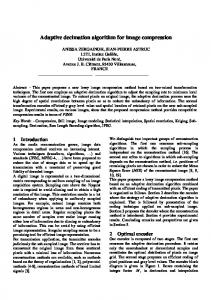
Figure 2: Degraded images in experiment and restoration comparison of three algorithms.
(a) Degraded image frame 1
(b) Degraded image frame 2
(c) Degraded image frame 3
(d) Degraded image frame 4
(e) Estimated PSF by our algorithm
(f) Restored image by our algorithm
(g) Restored image by RL-IBD algorithm
(h) Restored image by WeinerIBD algorithm
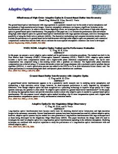
Figure 3: Multiframe original images and restoration comparison of three algorithms.
(2) According to the method of Section 2.2, for the initial PSF estimation ̂ℎ0 , normalized processing should be taken at same time. (3) Set the Max iteration of extrinsic cycles. (4) Set Max count of target and PSF estimation. (5) Set the inner loop counter variable h count by PSF estimation, variable f count of target inner cycle count.
Step 2 (the calculation of parameter values). (1) According to the formulas of Section 2.3, the variance 𝜎𝑛2 of mixed noise of each degradation image is estimated. (2) According to the method and calculation formulas from Section 2.2, calculate the power spectral density PSDℎ (𝑢) of PSF and estimate the wavefront phase error 𝜃𝑡 .
6
Abstract and Applied Analysis
250
150
200
100
150
Gray
Gray
200
50 0 150
100 50
100 Y( pix el)
50 0 0
50
100
0 0
150
0
50 100 Y (pi xel)
l) X (pixe
(a) Energy spectrum of observed image in Figure 3(a)
100
150 150
X
50 el) (pix
(b) Energy spectrum of our algorithm restored image in Figure 3(f)
200
250
150
200
100
Gray
Gray
250
50 0 150
150 100 150
50 100 Y (pi xe 50 l)
150 100 0 0
50
ixel) X (p
(c) Energy spectrum of RL-IBD algorithm restored image in Figure 3(g)
0 120
100
80
60 40 Y (pix el)
50 20
0 0
X
100 l) ixe (p
(d) Energy spectrum of Wiener-IBD algorithm restored image in Figure 3(h)
Figure 4: Energy spectrum of observed image and restoration comparison of three algorithms.
(3) According to the scheme and formulas of Section 2.4.1, estimate the regularization parameters 𝛼 and 𝛾(∇𝑥) of target edge. Step 3 (iterate calculation, 𝑖 = 0, 1, . . . , 𝑀𝑎𝑥 𝑖𝑡𝑒𝑟𝑎𝑡𝑖𝑜𝑛). (1) The inner loop count variable of PSF h count = 0. (2) The iteration process of PSF estimation 𝑗 = 0, 1, . . . , 𝑀𝑎𝑥 𝑐𝑜𝑢𝑛𝑡. ̂ (𝑖)
(a) Complete the PSF estimation ℎ with the conjugate gradient method using optimized formula (20). (b) Consider h count++; j++. (c) Judge the value of the loop variable 𝑗; if 𝑗 < 𝑀𝑎𝑥 𝑐𝑜𝑢𝑛𝑡, continue; otherwise, turn to (3). (3) The inner loop counter variable of target estimation 𝑓 𝑐𝑜𝑢𝑛𝑡 = 0.
(4) The iteration process of target estimation 𝑘 0, 1, . . . , 𝑀𝑎𝑥 𝑐𝑜𝑢𝑛𝑡.
=
(a) The conjugate gradient method was used to optimize formula (21) to complete target image estimation 𝑓̂(𝑖) ; (b) consider f count++; 𝑘 + +; (c) judge loop variable 𝑘; if 𝑘 < 𝑀𝑎𝑥 𝑐𝑜𝑢𝑛𝑡, continue; otherwise, turn to (5). (5) Judge whether the extrinsic loop is over; if it is 𝑖 > 𝑚𝑎𝑥 𝑖𝑡𝑒𝑟𝑎𝑡𝑖𝑜𝑛, then turn to Step 4. (6) 𝑖 = 𝑖 + 1, return to (1) and continue to loop. Step 4 (the algorithm is in the end). The cycle does not stop until the algorithm converges, and the output target image estimation is 𝑓̂ that is over.
Abstract and Applied Analysis
7
(a) Degraded image frame 1
(b) Degraded image frame 2
(e) Restored image by WeinerIBD algorithm
(c) Degraded image frame 3
(f) Restored image by RL-IBD algorithm
(g) Estimated PSF by our algorithm
(d) Degraded image frame 4
(h) Restored image by our algorithm
×104 8
×104 8
6 Gray
4
4
2
2
0 0
0 0
250
100 Y
(p 200 ixe l) 300
50
400 0
100
150
X
200
) xel (pi
(i) Energy spectrum of observed image in Figure 5(a)
Y
50 (p ixe l)
100 150
0
20
40
60
100
(j) Energy spectrum of our algorithm restored image in Figure 5(h) Wiener-IBD
0.7
80
ixel) X (p
0.8 RL-IBD Our algorithm
0.6 Intensity
Gray
6
0.5 0.4 0.3 0.2 0.1
(k) A line plot taken access the horizontal axis of image restored by Weiner-IBD, RL-IBD, and our algorithm
Figure 5: The multiframe observed stellar images and restoration comparison of three algorithms.
8
Abstract and Applied Analysis
3. Results and Analysis of AO Image Restoration Experiments
Table 1: Comparison of ΔSNR and 𝜀estimate values among three algorithms.
3.1. The Restoration Experiment on Simulate AO Images. The algorithm proposed in this paper is used to do the simulation experiment on degradation spot images; the evaluation of image restoration quality is judged by using root mean square error (RMSE) and improved ΔSNR. Consider
Algorithm name
RMSE = √
Wiener-IBD RL-IBD Our algorithm
1.982 3.046 4.164
3.62% 4.49% 5.10%
800 800 600
20.645 s 17.236 s 10.923 s
2 1 ∑(𝑓 (𝑖, 𝑗) − 𝑓̂ (𝑖, 𝑗)) , 𝑁1𝑁2 𝑖,𝑗
2 𝑔 − 𝑓 ΔSNR = 100 log10 . 𝑓̂ − 𝑓2
(22)
The evaluation of estimation accuracy is defined as follows:
𝜀estimate
ΔSNR (dB) 𝜀estimate Iteration Time-consuming
2 √ ∑𝑖,𝑗∈𝑆 ℎ(𝑖, 𝑗) − ̂ℎ(𝑖, 𝑗) ℎ = . √∑𝑖,𝑗∈𝑆 ℎ(𝑖, 𝑗)2 ℎ
(23)
In the formula, 𝑁1 and 𝑁2 represent the total number of pixels on 𝑥-axis and 𝑦-axis on the image, respectively. (𝑖, 𝑗) represents a pixel point on image, and 𝑓(𝑖, 𝑗) represents the gray value of the point (𝑖, 𝑗) on ideal image. In the simulation experiments of this paper, the original image is infrared simulation imaging with spots for multiple targets with long distance; 10 frames of simulation degraded image series are generated by image degradation software from the key optical laboratory of Chinese Academy of Sciences, and then add Gaussian white noise and make the signal-to-noise ratio SNR of image for 20 dB. Set parameters the same as adaptive optical telescope of 1.2 m on observatory in Yunnan. The main parameters of telescope imaging system are the atmospheric coherence length 𝑟0 = 13 cm, diameter of telescope 𝐷 = 1.08 m, comprehensive focal length of optical system 𝑙 = 22.42 m, the wavelength in center 𝜆 = 700 nm, and the pixel size of CCD is 7.4 𝜇m. Experiments on IBD algorithm based on RL iterative [16] (RL-IBD), iterative blind restoration algorithm based on the Wiener filtering [17] (Wiener-IBD), and the proposed algorithm are compared. Figure 2 is the compared results of the original image, simulated multiframe degradation images, and restoration images based on three kinds of algorithm; the image size is 217 × 218, Figure 2(a) is the original target image, and ten frames turbulence degraded image sequences are generated by using image degradation simulation software, as shown in Figures 2(b), 2(c), and 2(d) (to save space, we show only three frames; the rest is omitted); Figure 2(e) is the WienerIBD restored image, RMSE = 16.35; Figure 2(f) is the RLIBD restored image; the number of iterations is 800 times, RMSE = 10.31; Figure 2(g) is restored image used method in this paper, the variance of wavefront phase error 𝜃𝑡 (⋅) is 6.14 × 10⁻³ , ̂ℎ0 = 8.26 × 10⁻³ , and 𝜎𝑛2 = 1.1 × 10⁻⁵ that the regularization parameters in the experiments are 𝛼 = 1.25; the parameter of regularization function is 𝜉 = 1.34, extrinsic iterations for 100 times, inner loop of the PSF for 4, image
cycles for 2, namely, the total times of cycling is 600, RMSE = 10.05. Comparing with ΔSNR and precision from Figures 2(e), 2(f), and 2(g) are shown in Table 1. Comparison results show that the proposed algorithm in this paper is better than Wiener-IBD algorithm and RL-IBD algorithm and needs less time of iterations. 3.2. Restoration Experiments about Binary AO Images. Without the reference of ideal image, using the objective quality evaluation with no reference image, the Full Width Half Maximum (abbreviated as FWHM) [18] is used as objective evaluation for image restoration in this paper; FWHM refers to imaging peak pixels is two times of half peak, including the FWHM on 𝑥 direction and 𝑦 direction; for the better evaluation in astronomical observation areas, computation formula is shown as follows: FWHM = √FWHM 𝑥2 + FWHM 𝑦2 .
(24)
The experiment for the binary image restoration without reference images is carried out by the algorithm proposed in this paper. The binary images for experiments were taken by the 1.2 m AO telescope from Chinese Academy of Sciences in Yunnan observatory on December 3, 2006. The size for imaging CCD is 320 × 240 pixels array; the main parameters of imaging system are as follows: the atmospheric coherent length 𝑟0 = 13 cm, telescope aperture 𝐷 = 1.03, all imaging observation band is 0.7∼0.9, center wavelength 𝜆 = 0.72, the CCD pixel size is 6.7 𝜇m, and optical imaging focal length 𝑙 = 20. Recovery experiments based on RL IBD algorithm, Wiener-IBD algorithm, and the proposed algorithm in this paper are compared; the frame selection technology is taken in this paper; 40 frames are picked from 100 frames of degradation images as blind convolution images to be processed. Figure 3 is the comparison results of multiframe degraded images and restoration images based on three kinds of algorithms. Figures 3(a), 3(b), 3(c), and 3(d) are for the observation of the binary image (to save space, we show only four frames; the rest is omitted); Figure 3(e) is the estimation of the point spread function (PSF) based on the algorithm in this paper; Figure 3(f) is the restored image based on the method proposed in this paper; the variance of wavefront phase error 𝜃𝑡 (⋅) is 6.04 × 10⁻³ , ̂ℎ0 = 9.03 × 10⁻³ , and 𝜎𝑛2 = 1.32 × 10⁻⁵ so that the regularization parameter in this experiment is 𝛼 = 1.15; the parameter of regularization function is 𝜉 = 1.34, extrinsic iterations for 50 times, the inner
Abstract and Applied Analysis loop of PSF for 4 times, and image loop for 2 times, namely. The total times of iteration are 300, FWHM = 6.17 pixels, and the restoration results are very close to the diffraction limit of 1.2 m AO telescope; Figure 3(g) is the restoration result based on RL-IBD algorithm, FWHM = 5.62 pixels; Figure 3(h) is the restoration result based on Wiener-IBD algorithm, FWHM = 4.76 pixels. Figure 4 is the sketch of energy for the observation image and three kinds of restored images based on three restoration algorithms. With the comparison, it shows that the proposed algorithm in this paper is better than WienerIBD algorithm and RL-IBD algorithm and needs less time of iterations. 3.3. Restoration Experiments about Stellar AO Images. Also, the restoration experiment of stellar images was carried out using the algorithm in this paper; the stellar images for experiment were taken by 1.2 m AO telescope from the Chinese Academy of Sciences in Yunnan observatory on December 1, 2006 collection. The parameters of the optical imaging system are the same as that of binary images, and the method of parameters selection for experiments in this paper is nearly the same. Figure 5 is the comparison of multiframe stellar observation images and restoration results based on the three algorithms. Figures 5(a), 5(b), 5(c), and 5(d) are the observation of stellar images (to save space, we show only 4); Figure 5(e) is for the Wiener-IBD restored image; Figure 5(f) is the RL-IBD restored image; Figure 5(g) is the estimation of the point spread function (PSF) based on algorithm in this paper, the iterative initial value ̂ℎ0 = 9.56 × 10⁻³ , PSF iterative for six times; Figure 5(h) is the restored image based on algorithm in this paper; Figure 5(i) is the energy of the observed image for stellar; Figure 5(j) is the energy of restoration image based on the algorithm in this paper; Figure 5(k) is the graph of comparison results for three restoration algorithms.
4. Conclusions In this paper, according to the characteristic of adaptive optics image, we establish a degradation image model for multiframe exposure image series, and the mathematical model of the point spread function (PSF) for adaptive optical system after closed loop correction is derived; the PSF model based on phase error and changing over time is solved, and we use the power spectral density of image and constrain support domain method for AO image denoising processing. Finally, this paper applied the actual AO imaging system parameters as prior knowledge combined with regularization technique to improve the EM blind deconvolution algorithm. Experimental results show that the established blind deconvolution algorithm based on improved EM method can effectively eliminate the atmospheric turbulence and eliminate the noise pollution brought by the AO closed-loop correction, which improves the resolution of the adaptive optical image. The image process of AO observed images shows that the restoration quality is better than the same kind of IBD algorithm. It also shows that the restoration of binary images using the algorithm of this paper has carried on
9 the identification of PSF and completed the AO image after processing; the results of actual AO image restoration have important application value.
Conflict of Interests The authors declare that there is no conflict of interests regarding the publication of this paper.
Acknowledgments This project is supported by the Scientific and Technological Research Project of Jinlin province, Department of Education, China (no. 2013145 and no. 201363), and the basis study project is supported by Jinlin Provincial Science & Technology Department, China (no. 201105055).
References [1] J. Wenhan, “Adaptive optical technology,” Chinese Journal of Nature, vol. 28, pp. 7–13, 2005. [2] G. R. Ayers and J. C. Dainty, “Iterative blind deconvolution method and its applications,” Optics Letters, vol. 13, no. 7, pp. 547–549, 1988. [3] L. Dayu, H. Lifa, and M. Quanquan, “A high resolution liquid crystal adaptive optics system,” Acta Photonica Sinica, vol. 37, pp. 506–508, 2008. [4] C. Rao, F. Shen, and W. Jiang, “Analysis of closed-loop wavefront residual error of adaptive optical system using the method of power spectrum,” Acta Optica Sinica, vol. 20, no. 1, pp. 68–73, 2000. [5] B. Chen, The theory and algorithms of adaptive optics image restoration [Ph.D. thesis], Information Engineering University, Zhengzhou, China, 2008. [6] T. Yu, R. Changhui, and W. Kai, “Post-processing of adaptive optics images based on frame selection and multi-frame blind deconvolution,” in Adaptive Optics Systems, vol. 7015 of Proceedings of SPIE, Marseille, France, June 2008. [7] T. J. Schulz, “Nonlinear models and methods for space-object imaging through atmospheric turbulence,” in Proceedings of the IEEE International Conference on Image Processing, vol. 9, Lausanne, Switzerland, 1996. [8] L. Yaning, G. Lei, and L. Huihui, “Total variation based band-limited sheralets transform for image denoising,” Acta Photonica Sinica, vol. 242, pp. 1430–1435, 2013. [9] J. Zhao and J. Yang, “Remote sensing image denoising algorithm based on fusion theory using cycle spinning contourlet transform and total variation minimization,” Acta Photonica Sinica, vol. 39, no. 9, pp. 1658–1665, 2010. [10] C. L. Matson and M. C. Roggemann, “Noise reduction in adaptive-optics imagery with the use of support constraints,” Applied Optics, vol. 34, no. 5, pp. 767–780, 1995. [11] D. W. Tyler and C. L. Matson, “Reduction of nonstationary noise in telescope imagery using a support constraint,” Optics Express, vol. 1, no. 11, pp. 347–354, 1997. [12] L. Zhang, J. Yang, W. Su et al., “Research on blind deconvolution algorithm of multiframe turbulence-degraded images,” Journal of Information and Computational Science, vol. 10, no. 12, pp. 3625–3634, 2013.
10 [13] A. P. Dempster, N. M. Laird, and D. B. Rubin, “Maximum likelihood from incomplete data via the EM algorithm,” Journal of the Royal Statistical Society B, vol. 39, no. 1, pp. 1–38, 1977. [14] L. M. Mugnier, J. Conan, T. Fusco, and V. Michau, “Joint maximum A posteriori estimation of object and PSF for turbulencedegraded images,” in Bayesian Inference for Inverse Problems, vol. 3459 of Proceedings of SPIE, pp. 50–61, San Diego, Calif, USA, July 1998. [15] H. Hanyu, Research on Image Restoration Algorithms in Imaging Detection System, Huazhong University of Science and Technology, Wuhan, China, 2004. [16] F. Tsumuraya, “Iterative blind deconvolution method using Lucy’s algorithm,” Astronomy & Astrophysics, vol. 282, no. 2, pp. 699–708, 1994. [17] S. Zhang, J. Li, Y. Yang, and Z. Zhang, “Blur identification of turbulence-degraded IR images,” Optics and Precision Engineering, vol. 21, no. 2, pp. 514–521, 2013. [18] B. Chen, C. Cheng, S. Guo, G. Pu, and Z. Geng, “Unsymmetrical multi-limit iterative blind deconvolution algorithm for adaptive optics image restoration,” High Power Laser and Particle Beams, vol. 23, no. 2, pp. 313–318, 2011.
Abstract and Applied Analysis
Advances in
Operations Research Hindawi Publishing Corporation http://www.hindawi.com
Volume 2014
Advances in
Decision Sciences Hindawi Publishing Corporation http://www.hindawi.com
Volume 2014
Journal of
Applied Mathematics
Algebra
Hindawi Publishing Corporation http://www.hindawi.com
Hindawi Publishing Corporation http://www.hindawi.com
Volume 2014
Journal of
Probability and Statistics Volume 2014
The Scientific World Journal Hindawi Publishing Corporation http://www.hindawi.com
Hindawi Publishing Corporation http://www.hindawi.com
Volume 2014
International Journal of
Differential Equations Hindawi Publishing Corporation http://www.hindawi.com
Volume 2014
Volume 2014
Submit your manuscripts at http://www.hindawi.com International Journal of
Advances in
Combinatorics Hindawi Publishing Corporation http://www.hindawi.com
Mathematical Physics Hindawi Publishing Corporation http://www.hindawi.com
Volume 2014
Journal of
Complex Analysis Hindawi Publishing Corporation http://www.hindawi.com
Volume 2014
International Journal of Mathematics and Mathematical Sciences
Mathematical Problems in Engineering
Journal of
Mathematics Hindawi Publishing Corporation http://www.hindawi.com
Volume 2014
Hindawi Publishing Corporation http://www.hindawi.com
Volume 2014
Volume 2014
Hindawi Publishing Corporation http://www.hindawi.com
Volume 2014
Discrete Mathematics
Journal of
Volume 2014
Hindawi Publishing Corporation http://www.hindawi.com
Discrete Dynamics in Nature and Society
Journal of
Function Spaces Hindawi Publishing Corporation http://www.hindawi.com
Abstract and Applied Analysis
Volume 2014
Hindawi Publishing Corporation http://www.hindawi.com
Volume 2014
Hindawi Publishing Corporation http://www.hindawi.com
Volume 2014
International Journal of
Journal of
Stochastic Analysis
Optimization
Hindawi Publishing Corporation http://www.hindawi.com
Hindawi Publishing Corporation http://www.hindawi.com
Volume 2014
Volume 2014