Original data used in training the neural network (Hughes, Davis, and Davey). Latitude (fl) ... mathematical procedure for assigning weights to samples so that ...
Computers & Geosciences Vol. 19, No. 4, pp. 567-575, 1993 Printed in Great Britain. All rights reserved
0098-3004/93 $6.00 + 0.00 Copyright © 1993 Pergamon Press Ltd
RESERVE ESTIMATION USING NEURAL NETWORK TECHNIQUES XIPING WU and YINGXINZHOU School of Civil & Structural Engineering, Nanyang Technological University, Nanyang Avenue, Singapore 2263, Republic of Singapore (Received 29 June 1992; revised 3 November 1992) Abstract--Reserve estimation involves the modeling of spatial variation and distribution of ore grade in the region of exploration. Current approaches are based essentially on either geometrical reasoning or statistical techniques, and generally assume that the spatial distribution of ore grade is a function of distance. Recent advances in neural networks have provided a decidedly new approach to solving this problem. In this paper, we describe our research in using a multilayer feedforward neural network to capture the spatial distribution of ore grade by directly training the network with field assay data at borehole locations. The trained neural network then is used to predict the distribution of ore grade in the drilling region. Results predicted from the neural network model are reasonably accurate compared with other conventional models. The main advantage of this approach is that it requires no complicated mathematical modeling and makes no assumptions about the spatial distribution of ore grade. This research indicates that neural networks are a promising tool in solving the generic reserve estimation problem in mining engineering. Key Words: Neural networks, Learning, Artificial intelligence, Ore reserve, Exploration, Mining.
INTRODUCTION The distribution of ore grade is determined by many factors in the complicated geological process which led to the deposit of the orebody. Many of these factors are not known and cannot be brought into a traditional mathematical model. Any attempt to model ore grade distribution inevitably requires simplification and assumptions of the spatial variation. In almost all ore reserve-estimation methods, it generally is assumed that the ore grade is a function of distance. Usually this is the only factor considered. Other factors include geological structure, deposition environment, type of deposit, type of ore, and degree of mineralization, etc. Recent advances in neural networks, especially new insight into learning algorithms, have facilitated the development of a decidedly different approach to the estimation of ore grade and subsequently the estimation of ore reserve. The attractiveness of neural networks lies in the fact that they are not only trainable nonlinear dynamic systems, but also adaptive model-free estimators for nonlinear function estimations. With this approach, no assumptions need to be made about any factors or relationships concerning the spatial variation of ore grade in the vicinity of boreholes. Rather, the network is presented directly with the field assay data at borehole locations for training. Given sufficient data and appropriate training, the network can be taught to recognize the relationship between patterns of input (coordinates) and patterns of output (e.g. ore
grade) and then generalize to interpolate ore grades for areas between boreholes. In this paper, we present the results of our research in using adaptive feedforward neural networks as a computational tool to capture the relationship in spatial distribution of ore grade for copper reserve estimation.
CURRENT TECHNIQUES There are various techniques for ore-reserve estimation. No detailed discussion is necessary as these methods are well documented in the literature (Popoff, 1966; Barnes, 1980). Instead, for comparison purposes, we give a brief review on several more widely used ones, illustrated through an example from Hughes, Davis, and Davey (1979). All results based on the current techniques are from the same example. The example estimates the grade based on drillhole composites for a level in a surface copper mine with an assumed bench height of 12 m (40 ft). Drillhole locations and corresponding grades are shown in Figure 1, and original data extracted from the example are presented in Table 1. A maximum radius of influence of 76.2 m is applied. Polygon method The polygon method is the most widely used method, especially before the wide availability of computers. The weight for overall estimate is determined by the tonnage of the polygon that surrounds
567
568
X. Wu and Y. ZHOU ~O
I
oc-zo 0.17S
C 21A 13 ~)~417
0C-22 0.215
_¢-2! U0.489
C - ~ r t C-24 cIC-120.37700.427C-13 OO.31~ 0.1~1§
n C-14 0.140
I nC-~M~ i~C-15 t~C-19
~C-39 oC-37 -- ~ 2 - - 0 . 3 2 0 - - 0 . 7 1 7
.= o
rtC_25 0.230
o
C-40 OOJOZ
ff
~
nC-58 -- 0,806--0.889-- 0.4 7~) I C--28_C-27 _ C - I _ G - I T _C--Z _C-13 C_-19 I.I U I u 0.719 KIt.OOI U 0 . 8 ~ U 0,089 U
0.83~ 0.453 /
C-41
O.09Z I
C-(J(
C
~
C-42
C-9
0
C-49
C-IO
C-44
0
c-7 0.ot3°~.3~ 0.~s L~35~ 4 o °o.'44 c-Ls c-s c-z~ c-. c - s o c-Ls O|o61S O 0 . ~ S O 0.4Gsr~o.o~ 4 oC-Z9 C-tt~ O 0 . z ~ O ~ 0.476 0 0 . 4 0 9
I Q C - 4 7 o C - 6 1 QC-48 D C - 4 ~ QC-40 0.165 0 . 0 ( ~ 0 , 4 0 6 0.909 0.012
cIC-51 0.220
C-23
C-4
C-5S
e-5
o o.zz4ao~moa o;o~a o . ~ C-S5 n O.ZZ5
0
300
600
Departure, meters Figure 1. Assay composites with hole numbers and percent copper (after Hughes, Davis, and Davey, 1979). a particular sample. If the method is used locally to predict the grade at a point, the weight is simply one for the closest sample and zero for all others. Figure 2 shows the polygons drawn for the area of interest (Hughes, Davis, and Davey, 1979). The total tonnage, assuming a unit
weight of 2.58 t/m 3, is shown in Table 2. Inverse distance method
The inverse distance method estimates the grade at a point by assuming that weights are inversely proportional to some power of the distance between a
jo :0:0:0:18:18:i6:18 ;42:42i49:49:49:0:0:0:0:0:0:0' t" t. 4. 4. 4' 4. 4. 4. 4. 4.. 1. 4. t' t. 4. 4. 1. 4. 4. 1. | 0 0 0 0 18 18 18 4 2 4 2 4 2 1 4 9 4 9 4 9 0 0 0 0 0 0 0 1" 4- -I. 4- 4. 1' 1" ÷ 4. 4. "1' 1. 4. ÷ t- 4. 4. 4. 4. 1. 12121 21 21 4018 1 8 4 2 4 2 4 2 1 4 9 4 9 4 9 1 4 1 4 1 4 1 4 0 0 0 t._
4.
4.
4.
4.
4.
~
12, al z, 2, 4 0 4 0 ~ 3 o 1" 4. 1. .I- 1. ÷ 4~',~'~1"
4 . ~
1.
4.
4.
.4. 4.
4.
1"
÷
~
,
~143.3 4 3 , 4 , 4 i, ,4 o o o 4. ÷ 4. + -4" 4. 4- 4- ÷ ,
4, t "
121 21 21 21 40401:1~9.~.~113838~4343 43 14 14 14 14 0 0 0
t/)
to 4-04-~o°,o"~'~~4dg~'~'~'~J,'J~9
4"9% %
/0.0 I0 I0 tO lOiS 12 | ~ . ~ ~ . i ~ 2 1 7
7 4 4
0:0 ;lO~,O~a~.~,~, ~~?~~7.7
"o
44,4
t~
,.d 4-
1.. tl-
1.
4,
4.
1. 4-
4.
.
.
.
~'~
01.0 4 a ~ 1 . z 3 ~ 4~4.~7jr j 7 .~ 4.s 4 0 4 . 4 0 1 ~ ; j
4.
-t
4-
4-1.~ .o
0 4"0 ÷ 0 4-23 4 234.23•23 4.~94.9")4:~'~19 19 4' 3 ~ 3 '1.3939 I 4. 14.14.0i ,, t" 44" 0 0 0 ~ 2 3 2 3 ~ 2 2 2 2 2 2 t 9 19 3 3 3 9 3 9 3 9 0÷00!4-~ • 4. 41. 4, 4. 4. 4. ,I. t" .!, , , 4. 4. ~ 4. 4. * ÷ 0 4.O"1.0 4.0 4.0 ,I-0 ~,0 4.22~-224.22• 2,34"2,34"3* 3 4.39÷394.39÷0 +0 4.0 0 0 0 0 0 0 0 0 0 Z323~3230
C~
4. .0:0
0
~ 4- 4. 4. 41- 4- 4. 4. ., 4. 0 0 0 0 0 0 0 2 ~ . 2 ~ , 2 ~
0 0 0 0 00]
4. 4. ~. 4. 4. 2 ~ , 0 0 0 0
300
4;0.4"0.,4"0 t.
600
Departure, m e t e r s Figure 2. Computer-generated polygons from composited samples in Figure 1 (after Hughes, Davis, and Davey, 1979).
569
Reserve estimation using neural network techniques Table 1. Original data used in training the neural network (Hughes, Davis, and Davey) Latitude (fl) Departure (t~) Copper (%) 1900 600 0.175 1800 800 0.417 1800 1100 0.489 1600 220 0.215 1600 500 0.396 1600 700 0.685 1600 900 0.377 1600 1100 0.427 1600 1500 0.14 1400 300 0.392 1400 500 0.32 1400 690 0.717 1400 900 0.806 1400 1100 0.889 1400 1300 0.475 1200 500 0.23 1200 800 0.833 1200 900 0.453 1200 1100 0.719 1200 1300 1.009 1200 1500 0.893 1200 1700 0.089 1200 1900 0.092 1100 400 0.102
sample point and the point under consideration. It gives importance to more than one sample in the valuation of a block, with the inclusion of surrounding samples being limited by a predetermined radius of influence. Although this method seems to be an improvement over the polygon method, the selection of weights (power for distance) may be determined by trial-and-error and to a large degree depends on experience. The estimated block grades given by Hughes, Davis, and Davey (1979) are shown in Figure 3.
Latitude (fl) Departure (ft) 1000 1100 1000 1300 1000 1500 1000 1700 1000 1900 900 500 800 900 800 11O0 800 1300 800 1500 800 1700 800 1900 720 380 700 600 600 900 600 11O0 600 1300 600 1500 600 1700 500 500 400 900 400 11O0 400 1300 400 1500
Copper(%) 0.915 1.335 0.519 0.072 0.04 0.644 0.258 0.638 1.615 0.765 0.465 0.034 0.476 0.409 0.165 0.063 0.406 0.993 0.012 0.228 0.224 O.188 0.027 0.395
Geostatistical method The theory of geostatistics generally is defined as the application of regionalized variables to the study of ore reserve. This theory, formalized by Matheron in 1962, is recognized widely throughout the world to be a superior method for estimating grade of in situ mineralization (Barnes, 1979). Typically, the method has two basic steps: variogramming and kriging. The first step is a statistical treatment of the directional interdependencies of
Table 2. Comparison of methods for ore reserve estimation* No. of Blocks Cut-off Grade, %
0.60
Hand Polygon
........
Computer Polygon
66
Inverse Distance
Tons of Ore
0.55
0.60
Average Grade 0.55
0.60
0.55
1,804,836
1,804,836
0.93
0.93
66
1,844,637
1,844,637
0.92
0.92
65
69
1,816,687
1,928,484
0.91
0.89
Kriging
68
71
1,900,534
1,984,382
0.86
0.85
Neural Network
61
72
1,679,407
2,012,331
0.87
0.83
*All data based on Hughes, Davis, and Davey (1979) except for neural network. CAGEO 19/4--43
570
X. Wu and Y. ZHOU
,.d
0
300
600
D e p a r t u r e , meters Figure 3. Inverse distance interpolation from composited samples in Figure 1 (after Hughes, Davis, and Davey, 1979). sample grades, whereas the second step, kriging, is a mathematical procedure for assigning weights to samples so that the point estimate error is minimized. Figure 4 shows results of the block estimates by using the kriging method. This is by far the most complicated method in terms of mathematical manipulations and computation. The definition of the experimental variograms (curve fitting) is the most critical part and is highly dependent on the modeler's experience. NEURAL NETWORKS
A neural network is a nonlinear dynamic system consisting of a large number of highly interconnected processing units or processors. Its architecture and operations are inspired by our understanding and abstraction on the biological structure of neurons and the internal operation of the human brain. In a neural network, there are basically two major physical components: processing units or neurons and connections between these processing units. Each processing unit, acting as an idealized neuron, receives input, computes an activation, and transmits that activation to other processing units. The continuous McCulloch-Pitts computational model of the neuron (McCulloch and Pitts, 1943) is the most widely used one in multilayer feedforward neural networks. Associated with each connection between these processing units, there a weight value is defined to represent the connection strength, which acts as a
multiplicative filter together with the activation. Learning occurs while modification of a weight matrix is undertaken. Therefore, what the network computes is highly dependent on how the units are interconnected and the strengths of the connections or weights between them. It is through the presentation of examples, or training cases, and application of the learning rule, that a neural network obtains the knowledge or relationships embedded in the data. The propagation of activation in a neural network can be feedforward, feedback, or both. In a feedforward network, activations can be propagated only in a forward direction, whereas in a network with feedback mechanism this type of signal can flow in either direction. The network topology, the computational model of the neurons, the form of the rules and functions for activation propagation and computation, and the learning algorithms are all parameters in a neural network learning system, and lead to a wide variety of networks (Rumelhart and others, 1986). To date, the most well known and the most widely used network in applications is termed the backpropagation neural network developed by Rumelhart, Hinton, and Williams (1986) through backpropagating errors seen on the output processing units. The so-called generalized delta rule is the learning rule (Rumelhart, Hinton, and Williams, 1986). Curently, the computational capability of neural networks, especially multilayer feedforward networks, and their intrinsically parallel structure and
Reserve estimation using neural network techniques
571
0 '4,0 0 " 0 " 1 8 " 1 8 " 1 8 " 0 ' 0 " 0 0 : 0 " - 0 " - 0 : 0 : 0 : 0 " 0 ; 0 4" 4" 0 0 0 ÷01.01"18~181"18+4'242*4g 4g~4g~O ÷0 1"0 ÷0 "0 ÷0 0 0 ÷ 4 1. ÷ 4- 4- ÷ • ÷ 0 0 0 0 1818 ~04~4~494~4g0÷01"01"0÷01"01"0 *0 21. 21 ÷ 21 *40+40.~52 +58 1.53÷39442i45~'451"0" 14 *14+14* 0 '~0 + 0 ÷ 0 21:21:21;, >o>o--
0 0 ÷48.35÷31 ÷2g.41~.17 17 .17 6 . 6 1.40,40100:IOC I + I + 0 . 0 0 0 0 ?.3 2323 0 20201g 1515 15 ?.45950 I I 0 0 +
~.
4.
4.
4.
4-
÷
4-
:.>.io;o:o :o
÷
o o,o ooo 0
0 0 0÷0.,.01.0.0+0.23 0 0 0 0 0 23'
211"194" 3 ~ 19 4.39 1"39 4. 0 + 0 t " 0 .4. 0 23?.300000000
0"01.0"0 0
0
300 Departure,
600 meters
Figure 4. Kriging interpolation from composited samples in Figure 1 (after Hughes, Davis, and Davey, 1979). operation have been well recognized. Detailed description of the theory of neural networks, different learning architectures, and their learning algorithms are given in many books published recently (e.g. Hertz, Krogh, and Palmer, 1991). With new development in learning algorithms, the perspective on this computational model, which is capable of learning to discover hidden relationships in data, seems bright and promising. In the following section, we describe the development of an adaptive simulator for multilayer feedforward neural networks which is used in this study. ADAPTIVE SIMULATION OF MULTILAYER FEEDFORWARD
NETWORKS
In a neural network modeling process, the determination of learning process usually consists of two major aspects: the selection of a learning algorithm and the determination of the neural network architecture. The standard backpropagation neural network, has been demonstrated to be effective in learning, but is notoriously known to have a slow learning convergence rate because the generalized delta rule is basically a steepest descent scheme with constant step length in a network setting. Furthermore, the usual approach to architecture determination uses trial and error. This may only work for simple problems. For real-world engineering problems, it is imperative to have adaptive or dynamic mechanisms to determine the network architecture.
Recently, many learning algorithms and procedures were proposed to improve the modeling capability and learning convergence rate of the standard backpropagation neural network with the generalized delta rule (Becker and Le Cun, 1988; Fahlman, 1988; Jacobs, 1988; Moody, 1989) and to provide a mechanism for the determination of network architecture (Ash, 1989; Fahlman and Lebiere, 1990; Tenorio and Lee, 1989). A simple but fast learning rule termed the quickprop algorithm (Fahlman, 1988) and a straightforward scheme for estimating the size of hidden layer termed the Dynamic Node Creation (DNC) scheme (Ash, 1989) are shown to be effective and reliable. To facilitate an efficient determination of network architecture and training process, an adaptive simulator called DQP--Dynamic Quick-Propagation (Wu, 1991) that implements the quickprop algorithm and a variant of the Dynamic Node Creation (DNC) scheme, was utilized in this study. The quickprop learning algorithm was proposed to improve the rate of learning convergence of the generalized delta rule with adaptive estimation on the momentum factor by using gradient information on the current and previous steps, with the main assumption that the error versus weight curve for each weight can be approximated by a parabola. When the momentum factor is included, the generalized delta rule for weight update developed by Rumelhart, Hinton, and Williams (1986) is of the following form: Aw(t) = --~ 8 E / C w ( t ) + ~ A w ( t -- 1)
X. Wu and Y. ZHOU
572
where ~ is the learning rate, fl the momentum factor, E the error function, and w the weight vector. Both the learning rate and momentum factor are assumed constants. In the quickprop learning algorithm (Fahlman, 1988), the formulae for weight update becomes: Aw(t) = - ~ c~E/Ow(t) +
OE/Ow(t) Aw(t - 1). OE/Ow(t - 1) - OE/~w(t)
Numerical experiments indicate that the quickprop algorithm is robust in learning, converges fast, and seems scaled-up well for large learning problems (Fahlman, 1988; Wu, 1991). Based on the theoretical conclusion that a threelayer feedforward network is a universal approximator (Hornik, Stinchcomebe, and White, 1989), Ash developed the DNC scheme (Ash, 1989) within a standard backpropagation network, by fixing the network architecture to three layers with one hidden layer, starting training with one hidden node, and keep adding one hidden node at a time during a certain training period until convergence in learning is realized. The criterion for adding a new hidden node is governed whether the currently estimated average error slope over a certain number of epochs is less than a predefined gradient tolerance termed the "trigger slope". Although this approach seems to be robust intuitively in determining an optimal architecture on the training of the encode/decode and some other simple benchmark problems (Rumelhart, Hinton, and Williams, 1986), the selection of the trigger slope tends to be problem dependent. Within DQP, a heuristic node adding rule was utilized during the preliminary stage of training, in which a trigger slope defined as a percentage of correct predictions out of the total training cases was implemented. When the error on about 80% of the training cases has been reduced to within the predefined error tolerance, the architecture adjusting then is controlled manually. The training process converges when both the maximum absolute error and the total error are reduced below their tolerances, respectively.
reproduce the borehole data it was trained on, but through generalization, it should be able to approximate or interpolate the ore grade at locations inside or in the neighborhood of the drilling region. The degree of accuracy depends on the comprehensiveness and representativeness of the training data (e.g. borehole spacing and distribution) and how well the network is trained. Technical aspects involved in the construction of a neural network-based model usually include: (1) problem representation, (2) architecture estimation, (3) learning process determination, (4) training of the neural network with training data, and (5) testing of the trained neural network with testing data for generalization evaluation. In this problem, the representation scheme is straightforward. The network is given a spatial position (x and y coordinates) as input and asked to estimate ore grade for that location as output. Therefore, the network architecture consists of two nodes in the input layer, and one node in the output layer. From past experience (Wu, 1991; Ghaboussi, Garrett, and Wu, 1990, 1991) and theory (Lippmann, 1987), it was decided that two hidden layers would be used in the network and full connections between nodes in adjacent layers were enforced. With the use of DQP, the hidden size in each hidden layer can be determined as the training progresses. The training process converges when either the root mean squared total error or the maximum absolute error on the training data set has been reduced to below a designated error tolerance. The final architecture of the neural network is shown in Figure 5. In the following paragraphs, we describe the data processing or scaling of the sample data, training, and testing procedures. Training
In a multilayer feedforward neural network, training refers to the iterative process involving the presentation of training data to the network, the invocation of learning rules to the modification of connection weight matrix, and usually, the evolution of network Ore Grade OutputLayer: 1 node
RESERVE ESTIMATION WITH N E U R A L NETWORKS
Hidde~LayerII 28 nodes
The modeling methodology
The basic strategy for developing a neural networkbased model of spatial distribution of ore grade in a region is to train a multilayer feedforward network on borehole data. If the location and number of boreholes cover a reasonable part of the region and the data obtained from the assay are sufficient, then the trained network would have sufficient information to characterize the spatial variation of ore grade in the region encompassed by the boreholes. Such a trained network not only would be able to
Hidden LayerI: 28 nodes
InputLayer:2 nodes X and Y Coordinates
Figure 5. Architecture of neural network model.
Reserve estimation using neural network techniques architecture, such that the relationship embedded in the data is appropriately captured. Because of the use of the sigmoidal activation function, the original sample data need to be scaled to within the range of activation values defined by the sigmoidal function. In this study, all the input and output data are scaled linearly into the range of [0.0, 1.0], and training data then are prepared according to this representation scheme. For this example, the set of training cases is composed of the sample values from 51 boreholes (Fig. 1). At the onset of training, 4 nodes were used in each hidden layer, and the training process was considered eventually satisfactory when the root mean squared total error was reduced to below 0.09. The final hidden size for each hidden layer was increased to 28 nodes when the learning convergence tolerance was satisfied. However, it was observed that the maximum absolute error for data at two boreholes was yet about 0.26 even though that error for over 80% of the training cases was reduced to below 0.10. This indicates that either the sample data at the two boreholes were of large sampling error or the pattern at these two locations did not fit into the trend or internal relationship captured by the network. The training result is represented in Figure 6, in which the sample values are plotted against the predicted values from the network. It is obvious from the figure that the network has 0 ~D
573
1.75 1.40
/
O
o//
1.05 o
0.70
0 0~/~0
o
o
0
°
; oo 0.00 6{[,0
'
i
,
,
0.00
0.35
0.70
1.05
1.40
Actual values Figure 6. Actual grade values vs values predicted by neural network. captured the correlation between the location and ore grade of boreholes in the sampling data.
Testing After the network has learned the pattern of grade distribution based on the samples, estimates on ore grade for all the blocks in the level were made using the same block size given in the cited example. The
01946
49393330313234
36353121
8
0
0
3
7
8
01438
45393635363839
40 38 31 19
7
2
4
9 i0
8
0 II 32 3 9 3 9 3 9 4 0 4 2 4 4 4 5
45413219
9
8121412
0
926
34374146495151
5044332216182017
ii
5
0
923
28334351565858
5548372928302618
9
3
0
923
25284256646766
6265
7
1
0
925
24243757i717675
7164606160483014
5
0
0
929
28213054:746384
6178808274522912
3
0
3623234471716791
46 42 43 40 29 17
7
i
6
0
9294101102855527
0
632
0
232
0
026
0
016
0
0
4 38[~532912
816
0
0
0 1851 [6114521
5
1.75
ii
2
0
94 58 27 i0
1
0
.~9 ii
2
0
3112
3
0
48~382111412210469 3 5 1 5 6993916711918
4 7
0 0
9
2
00110120117
4531203053~ 4578193 52 44 25 19 60 83 0 1 1 1 9 1 3 1 1 2 7 1 0 2
61
50 57 37 19 16 28 52 8 3 1 1 3 1 3 2 1 3 0 1 0 6 6 6
1
i
0
1
8
5
512253841342212
27 51 163, sG 39 21
0
0
0
12751533615
i0
0
0
0
42643432813
0
0
0
0
0
319313224
15 ii 1 2 1 8 2 6 3 0 2 9 2 3 1 4
0
0
0
0
0
0
0 i02024
221917192327272417
0
0
0
0
0
0
0
0
312
18212222242728262114
0
0
0
0
0
0
0
0
0
0
4 7 i0
5121821242627272520
0
300
Departure, meters Figure 7. Block estimates using neural network model.
600
574
X, Wu and Y. ZHOU
results are shown in Figure 7. The total number of blocks with estimated Cu grade >0.6% is 61, with an average grade of 0.87% (Table 2). The network yielded fewer blocks with grades />0.6% Cu. However, a closer examination of the block grade distribution reveals that there are many blocks with grades close to 0.6% Cu. In fact, if all blocks that have a grade of at least 0.55% Cu are counted, the total number of blocks would be 72, yielding a total estimated ore of 2,012,331 tons, compared to 71 blocks and 1,984,382 tons for kriging. For comparison purposes, block estimates based on a cutoff grade 0.55% Cu are also made for all other methods and are shown in Table 2. It is interesting to note that the network seems to have "learned" the fact that samples with high grades are few compared to those with medium grades. This can be seen from the fact that the network tends to under-predict for high grade values which have relatively few training cases (Fig. 6). Grades with higher frequencies of occurrence are given more importance. In a sense, the network itself also attempts to assign weights. These weights, however, are not for determining the influence of individual samples on a point, but rather are weights of individual samples in the whole model of the ore grade distribution. Note that for borehole C-27 (Fig. 1), which has a sample grade of 0.453%, whereas all samples surrounding it have grades >0.60%, the neural network simply ignored it, probably treating it as an outlier or a sampling error. This in practice makes more sense, especially considering the fact that ore grade distribution shows a continuity. Another interesting result is that the network was able to pick out a second "peak" in the grade distribution, which was represented by only one borehole, C-7. Furthermore, the predictions of the neural network on ore grade for blocks out of the training region seem to be in accordance with the general trend. This indicates that after appropriate training on a fairly comprehensive set of sample data, the network can generalize reasonably well in the neighborhood of the sampling region. DISCUSSION In the preceding analysis, it has been demonstrated that the neural network technique can be used successfully in reserve estimation. This technique requires no complicated mathematical modeling, except simple calculations performed internally by the network to arrive at its conclusions. It is a mapping process in which the network was trained to recognize the pattern in the ore grade distribution, in much the same way human beings would if they actually could visualize the spatial distribution. This method is not only simple, but also more reliable and is applicable universally to any spatial distribution of grade because it does not make any assumptions about the distribution. There are no weights to assign, no radius
of influence to assume, no models to fit about the variance, and no assumptions to make about the relationship between grade and distance (2- or 3-D). In addition, the influence of geological environments (unknown geological boundaries) are incorporated implicitly in the mapping process as the network "learns" the pattern of grade variation. If different geologic formations are known, they can simply be represented in the model by creating another variable in the representation scheme of input. In contrast, all interpolation techniques reviewed here assume that grade is related to distance. The influence of distance and direction are determined based on assumed weights and some functions. As a consequence, they are subject to uncertainties about the real functional relationship, whether this relationship changes from deposits to deposits, and from the influence of geological environments. As a first attempt to use the neural network techniques in ore-reserve estimation, some of the interesting observations are worth noting. The current network tends to scale down or up values which have a low frequency of occurrence to fit the model it builds. This may not be desirable in some applications when it is known that certain values are true and physically present, regardless of their frequency of occurrence. A possible way to solve this problem may be to force the network to learn and memorize these values in the initial stage of training and then fix or freeze a part of the network. This, however, was not carried out for our example because of the constraint of the current simulator. It will be addressed in our ongoing research in this direction. CONCLUDING REMARKS In this paper, it has been demonstrated that neural networks can be used successfully in ore-reserve estimation. With this approach, the spatial distribution of ore grade can be captured directly within the weight structure of a neural network through training on the sample data of boreholes. Subsequently, ore reserve for the region of interest can be readily estimated. On the other hand, the flexibility of representation scheme made it possible to include as many features as possible into the input and output of a neural network-based model. This neural network-based approach shows promise in solving the generic ore reserve-estimation problem in mining engineering. Although it generally is true that neural networks are not best suited for precise mathematical computations, they have superior capabilities in recognizing patterns and discover relations hidden in the sometimes noisy sample data. It can be envisioned that the best application of neural networks in engineering problem solving is in combination with traditional methods, rather than replacing them or using it as a stand alone system. In this connection, neural networks can be used in recognizing important patterns
Reserve estimation using neural network techniques in ore-grade distribution whereas the traditional methods then can be used for more precise calculations. Certainly there is also much work to be done in the area of network training, in forced learning, and in selecting the type of network that is best suited for ore estimation. REFERENCES
Ash, T., 1989, Dynamic node creation in backpropagation networks: ICS Report 8901, Institute of Cognitive Science, Univ. California, San Diego, La Jolla, California, lip. Barnes, M. P., 1979, Drillhole interpolation: estimating mineral inventory, in Crawford, J. T., and Hustrulid, W. A., eds., Open pit mine planning and design: AIME, New York, p. 65-80. Barnes, M. P., 1980, Computer-assisted mineral appraisal and feasibility: AIME, New York, 167 p. Becker, S., and Le Cun, Y., 1988, Improving the convergence of backpropagation learning with second order methods, in Touretzky, D. S., Hinton, G., and Sejnowski, T., eds., Proc. 1988 connectionist models summer school: Morgan Kaufmann Publishers, San Mateo, California, p. 29-36. Fahlman, S. E., 1988, Fast learning variations on backpropagation: an empirical study, in Touretzky, D. S., Hinton, G., and Sejnowski, T., eds., Proc. 1988 connectionist models summer school: Morgan Kaufmann Publishers, San Mateo, California, p. 38 51. Fahlman, S. E., and Lebiere, C., 1990, The cascade-correlation learning architecture, in Touretzky, D. S., ed., Advances in neural information systems II: Morgan Kaufmann Publishers, San Mateo, California, p. 524 532. Ghaboussi, J., Garrett Jr., J. H., and Wu, X., 1990, Material modelling with neural networks, in NUMETA 90: Proc. Intern. Conf. numerical methods in engineering: theory and applications, Swansea, U.K., p. 701-717. Ghaboussi, J., Garrett Jr., J. H., and Wu, X., 1991, Knowledge-based modelling of material behaviour with neural networks: Jour. Engineering Mechanics, ASCE, v. 117, no. I, p. 132-153.
575
Hertz, J., Krogh, A., and Palmer, R. G., 1991, Introduction to the theory of neural computation: Addison-Wesley Publ. Co., Redwood City, California, 327 p. Hornik, K., Stinchcomebe, M., and White, H., 1989, Multilayer feedforward networks are universal approximators: Neural Networks, v. 2, p. 359-366. Hughes, W. E., Davis, F. B., and Davey, R. K., 1979, Drill hole interpolation: mineralized interpolation techniques, in Crawford, J. T., and Hustrulid, W. A., eds., Open pit mine planning and design: AIME, New York, p. 51 64. Jacobs, R. A., 1988, Increased rate of convergence through learning rate adaptation: Neural Networks, v. 1, p. 295-308. Lippmann, R. P., 1987, An introduction to computing with neural nets: IEEE ASSP Magazine, p. 4-22. McCulloch, W. S., and Pitts, W., 1943, A logical calculus of the ideas immanent in nervous activity: Bull. Math. Biophysics, v. 5, p. 115 133. Moody, J., 1989, Fast learning in multi-resolution hierarchies, in Touretzky, D. S., ed., Advances in neural information processing systems I: Morgan Kaufmann Publishers, San Mateo, California. Popoff, C. C., 1966, Computing reserves of mineral deposits: principles and conventional methods: U. S. Bur. Mines, Inform. Cir. 8283, Government Printing Office, Washington, D.C., 29 p. Rumelhart, D. E., McClelland, J. L., and the PDP Research Group, 1986, Parallel distributed processing: exploration in the microstructure of cognition, v. 1: foundations: The MIT Press, Cambridge, Massachusetts, 547 p. Rumelhart, D. E., Hinton, G. E., and Williams, R. J., 1986, Learning internal representations by error propagation, in Rumelhart, D. E., and McClelland, J. L., eds., Parallel distributed processing, v. 1: foundations: The MIT Press, Cambridge, Massachusetts, p. 318 362. Tenorio, M., and Lee, W.-T., 1989, Self-organizing neural network for optimum supervised learning: TR-EE-8930, School of Electrical Engineering, Purdue Univ., Indiana, 42 p. Wu, X., 1991, Neural network-based material modelling: unpubl, doctoral dissertation, Dept. Civil Engineering, Univ. Illinois at Urbana-Champaign, Urbana, Illinois, 202 p.