Reservoir Computing with Random Skyrmion Textures

Reservoir Computing with Random Skyrmion Textures D. Pinna,1 G. Bourianoff,2 and K. Everschor-Sitte1 1

Institute of Physics, Johannes Gutenberg-Universit¨ at, 55128 Mainz, Germany 2 Intel Corp., retired (Dated: December 13, 2018)

The Reservoir Computing (RC) paradigm posits that sufficiently complex physical systems can be used to massively simplify pattern recognition tasks and nonlinear signal prediction. This work demonstrates how random topological magnetic textures present sufficiently complex resistance responses for the implementation of RC as applied to A/C current pulses. In doing so, we stress how the applicability of this paradigm hinges on very general dynamical properties which are satisfied by a large class of physical systems where complexity and intrinsic material memory can be put to computational use. By harnessing the complex resistance response exhibited by random magnetic skyrmion textures, we explain how spintronically accessable magnetic systems offer a potential advantage in the search for an ideal reservoir computer. The ultra low-power properties of compact skyrmion fabrics, coupled with their CMOS integrability operating on similar length and timescales, open the door for their RC employment geared towards industrial application.

I.

INTRODUCTION

Motivation – It is widely acknowledged that classical Dennard scaling1 of complementary metal-oxide semiconductor (CMOS) logic, making devices simultaneously smaller, faster and operating at lower voltage, ceased at the turn of the millenium when transistor channel lengths reached the order of 100 nm. Subsequently, dimensional scaling of semiconductors continued in step with Moores law (with a two-year cadence), thus making devices smaller and cheaper. During that same period, a number of enhancements to CMOS were made to further improve transistor performance such as strained channels2 , high K/metal gates3 , steep subthreshold devices4 , trigate geometries5 , and high mobility channel materials6–8 . However, as we approach the theoretical limit of 3 nm transistor channel lengths9 manufacturing challenges become exponentially more difficult and more expensive to overcome. The increasing marginal cost of progressively smaller performance gains is expected to make further silicon scaling uneconomical. The latter is expected to occur within the next two fabrication generations with the advent of ∼ 5 nm transistor sizes. Simultaneously, a seismic shift is occurring in the computational workloads from data-based offline processing to real-time big data applications driven by the Internet of Things (IoT), robotics and autonomous agents. This combination of factors has led to a sudden exploration of alternative computing methodologies that span the entire Boolean computational stack from physical effects, to materials, devices, architectures, and data representations. It also includes novel non-Boolean methods of computing such as quantum, wave and neuromorphic computation, Boltzmann machines and others. Exactly which combination of computational elements will evolve from this plethora of options is far from clear. However, it is possible to state general requirements future computing platforms must meet. First, any new computing methodology must be compatible with the existing multi-trillion dollar infrastructure associated with cur-

rent CMOS based computing. Second, it must be scalable through multiple generations of incremental hardware and software improvements and, third, the performance/cost metric must exceed that of Boolean CMOS processors. One approach stems from the intuition that physical systems, governed by their underlying physical laws, effectively compute the evolution of their state in a natural way. More abstractly, matter implicitly stores the correlated physical information defining its dynamical state. It feeds back this information through its interacting environment such that both may modulate and respond to each other’s properties. If an experimentally observable physical system can be constructed whose spontaneous dynamics map into solutions of a given problem, we can state that the system’s matter has been used for computations. This paper will outline a specific physical system of such type. By combining the use of electron transport through random magnetic textures10,11 and the principles of reservoir computing12 , we will demonstrate the possibility of using magnetic systems as analog computers capable of processing and classifying data with complex correlational features. To stress the importance and generality of the principles employed, we now briefly review the salient properties allowing physical material systems to intrinsically compute starting from the success of deep neural networks (DNN). Deep Neural Networks – The most proficiently used machine learning technique geared towards heavy data processing and pattern recognition is the DNN framework13–15 . It has enjoyed wide acclaim for its ability to outperform humans in tasks previously considered unattainable by machines, going as far as beating the human world champion of the game ‘Go’16 . The most general class of DNNs, known as recurrent neural networks (RNNs) (see Fig. 1a), considers coupled neurons whose graph representation consists of cycles forcing information to feedback (or echo) throughout the network and fade over time17–19 . This basic property allows RNNs to exhibit complex temporal dynamic behavior in response

2

FIG. 1. General schematic of reservoir computing for (a) a recurrent neural network and (b) a material-based reservoir. (c) Example of a skyrmion fabric reservoir with locations of input (output) contacts identified by green (red) dots. The in-plane orientation of the magnetization is color coded and (d) shown in detail with arrows for a sample Bloch skyrmion identified by the red frame in (c). The spatially extended nature of such a magnetic system allows for tunability in the number of electrical contacts. This allows to control the dimensionality of the reservoir snapshot. A reservoir computing system consists of three building blocks, the reservoir, an input and an output layer.

to the interplay of the instantaneous driving inputs and the RNN’s implicit internal memory’s echoing of past input information. Whereas the universal approximation theorem for feedforward DNNs guarantees the faithful representation of any function20,21 , the RNN’s capacity to harness temporal correlations through their echo-state memories allows them to emulate universal Turing machines22 . This has far-reaching consequences as RNNs can be considered universal approximators of dynamical systems as a whole. What hasn’t received much attention are the pitfalls that such algorithms fall-in the moment their employment is required to massively scale to networks consisting of many large coupled layers. The topology of neural networks is largely restricted by the ability to effectively train the large number of weights that must be tuned for proper operation to take place. RNNs are particularly penalized as their training converges much more slowly (if at all) than simpler feed-forward networks due to the vanishing gradient problem 23,24 . Approaches to overcome this fundamental difficulty have been proposed in the form of custom modifications to the general RNN structure25,26 - known as long short-term memory (LSTM) networks - with widely recognized success in tasks such as handwriting27 and speech28 recognition. Furthermore, LSTM networks, have allowed the use of RNNs to enter mainstream use for specific voice recogni-

tion tasks on handheld devices29–34 . Nonetheless, these state-of-the-art algorithms still mainly require the use of general purpose computers, thus inheriting the energy and speed bottlenecks typical of the end-of-Moore-law scaling of transistor sizes35 . Special purpose integrated circuit implementations such as IBM’s True North chip, with its 65 mW/cm2 consumption36 , pale with the cerebral cortex’s 1 mW/cm2 consumption. Deposition techniques used in the fabrication of microelectronic devices constrain special purpose hardware devices by imposing heavy costs to scaling networks requiring many-tomany connections. It should also be noted that clock distribution, power distribution and data interconnection have significant impact on overall chip power dissipation and complexity. Last but not least, successfully trained DNNs still exhibit impractically long inference times (10−3 − 1 s 37,38 ), defined as the time between input submission and output reception. This requires that data must be processed offline, precluding the possibility to process large amounts of real-time data as is required by the Internet of Things, robotics and real-time control systems. Ultimately, these bottlenecks arise from the need to model, store and especially train the many synaptic weights and node activation functions across the numerous hidden layers in RNNs. It was however noticed that Hebbian training of RNNs mostly modified just the output weights linking the bulk of the network to the

3

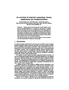
FIG. 2. Schematic of the reservoir computing operational principle. (a) Unstructured data from an input space is (b) nonlinearly projected by the reservoir’s transient dynamics onto its higher dimensional state space. Due to the similar evolution of the reservoir when driven similarly correlated input data samples (represented by similar colors), (c) a single linear regression step can be used to define hyperplanes in the reservoir’s state space such that different input data categories become separated. The task of the reservoir is to project different spatial-temporal events onto a sparsely populated high dimensional space where they become easier to recognize and categorize.

read-out layer39 . A related mechanism has also been observed in the modelling of sequence processing 40,41 and temporal input discrimination of biological neural networks42 . Reservoir Computing – These early works were the first to explicitly suggest the principle of reading out target information from a - mostly - randomly weighted RNN. They imply that a sufficiently large RNN can be potentially initialized with static random weights. Its training is then solely performed on a smaller set of weights associated with feed-forward connections between the bulk of the network and the output layer12,43–46 . Since such output weights consist of only a single layer connecting to the static RNN bulk (known as the reservoir ), the training is reduced to a linear regression performed on the reservoir state. The advantage of this method, now commonly referred to as Reservoir Computing (RC), is not earned for free as the reservoir network has to typically be topologically more complex than an equivalent RNN fully trained to perform an identical task. The principle supporting the feasability of this scheme lies in the purpose served by the large, static reservoir. Tasks such as pattern classification require the neural network to emphasize the data separation of, initially ambiguous, input patterns. A reservoir effectively performs a high dimensional nonlinear projection of the input data onto a large state manifold where the partitioning of the projected states is simplified via the introduction of hyperplanes (see Fig. 2 and Appendix A). The non-linearity

of this transformation, coupled with the RNN’s fading memory, will guarantee that the reservoir’s response to a given input will be sensitive to temporal correlations present in the input data which are comparable to the memory’s timescale. Distinct, but similarly correlated, input patterns will induce evolutions of the reservoir along similar trajectories. These trajectory bundles – known as phase tubes – corresponding to different input categories, rapidly separate from each other. The feedforward output layer effectively partitions the reservoir’s manifold via appropriate hyperplanes such that each individual phase tube can be unambiguously separated. Furthermore, since the network’s reservoir is not modified after initialization, a sufficiently complex reservoir can be used to process different input datasets independently of how they are structured47 . Each dataset will then solely require the training of a new, dedicated, output layer without modifying the reservoir itself. Whereas the RC approach appears to significantly simplify the training complexities of RNNs, the need for a potentially much larger network reservoir will exacerbate the computational resources and inference time requirements needed for proper modelling to take place. However, since the reservoir is only a static complex nonlinear dynamical system, it is not necessary for it to be implemented in the form of a DNN. Any sufficiently nonlinear and high dimensional analog physical system can in principle perform the same role48 . This paradigmatically different approach to computing - known as in-materio computing - seeks to overcome the digital limits of neural network modelling by leveraging the vast amounts of readily accessible physical complexity already present in nature (for a review see22 ). Following initial demonstrations involving single non-linear dynamical nodes with delayed feedback49 , recent work has explored the RC approach using physical systems ranging from liquid crystals50 , to water buckets51 , bacterial colonies52 , memristors53 , optical resonators54–57 and poly-butyl-methacrylate mixtures58–60 . In magnetic systems, single spin-vortex nano oscillators have been used to demostrate spoken digit recognition within the RC framework61 and skyrmions suggested for further RC development10,11 . The reservoir computing paradigm provides scientists with a generic and powerful tool to tackle tasks that require temporal dependencies, without employing hand-crafted data representations. Generally speaking, a performant reservoir has the following properties: 1. The dimension of the reservoir’s phase space must be much larger than size of the input category set. 2. To guarantee reproducibility of its dynamical responses to identical inputs, the reservoir has to relax or be resettable to the same initial state once all inputs are removed. 3. To ensure that memory of features fully affects the reservoir’s evolution, any temporal feature correlations present in the input data must be of the same

4 order as the natural transient dynamical timescale of the reservoir. 4. Reservoir dynamics must be nonlinear but not ergodic to the point of strongly mixing trajectories throughout reservoir evolution. 5. To properly identify all desired feature categories, a sufficienlty large enough subspace of the reservoir state should be measurable. The last requirement is particularly important in light of the dynamical systems interpretation used to justify reservoir computing. The feasability of exploiting a physical system as a reservoir intimately depends on the technical ability to reliably inject input data and sample a sufficiently high dimensional subspace of the reservoir’s intrinsic phase space. In fact, to capture the reservoir’s separation of N phase tubes corresponding to the number of input data categories, the output layer should be capable of generating a sufficient number hyperplanes to distinguish each phase tube pair. Since a properly functioning reservoir is input data agnostic, any device implementation must have the flexibility of tuning the dimensionality of the output layer to effectively classify diverse data sets. Many of the reservoir computing examples presented in the literature do not allow such tunability49,56,61–63 , choosing instead to employ multiplexing techniques to bypass the handling of both the input data and the reservoir state at such dimensionalities. This is also necessary whenever the input data’s temporal correlations are widely different from the reservoir’s natural timescales and need to be preprocessed in such a way as to properly excite the reservoir. With regards to the input data, this approach requires an extra preprocessing step to suitably mix the input data features together. This is often itself a nonlinear transformation of the input data. Similarly, in the output step, one samples a temporal trace of a coarse-grained sample of the reservoir’s state whose dimensionality is low compared to the dimensionality of the input categories. This is in contraposition to taking a high dimensional snapshot of the reservoir’s state at a fixed moment in time for nonmultiplexing techniques. The time trace values are then used to artificially boost the dimensionality of the readout without actually exploiting the potentially very high dimensional nature of the reservoir’s state space itself. In the two multiplexing steps presented, it is often unclear how much of the classification work has been performed by the reservoir as opposed to the nonlinear input data preparation and time trace measuring performed by the output layer61 . An ideal reservoir design should allow for arbitrary tunability of the dimensionality of both the input and output layers. This would, in turn, allow for a true RC implementation where unstructured data may be injected without any preprocessing and the reservoir state sampled via instantaneous, real-time, snapshots. Magnetic systems as Reservoirs – There is no dearth of physical systems in nature which satisfy the

general properties just discussed. Assessing, however, which systems may be industrially viable is an entirely different challenge. This work argues for the employment of magnetic textures due to their nanometer sizes, intricate dynamical properties and, most importantly, low-power and CMOS-compatible all-electrical operability. In particular, we study using random topological magnetic textures – skyrmion fabrics – to generate complex, high-dimensional representations of input voltage signals. Magnetic skyrmions are compact and metastable magnetic structures predicted over two decades ago64 and very actively studied experimentally both in lattice65 and isolated form66 . The particle-like properties of skyrmions have been extensively summarized in several reviews67–70 . Their mobility under ultralow current driving71,72 and room-temperature stability73–78 have garnered them a central position as information carriers in many device-relevant materials and applications79–83 . Device oriented research has however mostly ignored intermediate skyrmion phases – known as “skyrmion fabrics”10,11 – which interpolate between single skyrmions, skyrmion crystals and magnetic domain walls84 (an example is shown in Fig. 3b). We claim that the random phase structure, complexity, nonlinear response, and fading memory characteristics present in skyrmion fabrics justify their use as a RC reservoir. Gigahertz voltage patterns exciting the texture via nanocontacts can implement the injection of input information while the coupling of electron transport and magnetoresistivity85–87 can be used to sample the magnetic state of the system. The remainder of the paper is structured as follows. Section II will introduce our physical model in detail and argue how the interplay of sensitivity to driving currents, magnetoresistance and intrinsic memory effects can be harnessed for RC applications. We do so by discussing the importance that the delay between current density and magnetic relaxation plays on defining memory in the magnetic system. Section III will outline the numerical simulation of the models presented and verify both the non-linear processing performed by the skyrmion fabric on sample input signals as well as confirm the role played by the different natural timescales on the emergence of memory in the system. In conclusion, Section IV will further discuss the flexibility of our proposed design and reiterate the attention that should be directed towards exploring novel reservoir systems in nature.

II.

SKYRMION FABRIC RESERVOIR MODEL

For the sake of simplicity, we consider a random magnetic skyrmion phase in a spatially extended rectangular geometry with only two voltage contacts. To model a realistic setup, our sample is subject to DzyaloshinskiiMoriya interaction(DMI) via grain inhomogeneities and a static applied magnetic field (see Fig. 3 and Methods Section). A random magnetic texture is generated by im-

5

FIG. 3. (a) Randomly generated DMI-grain inhomogeneities employed to pin skyrmions. Figure shown corresponds to a 250-by-500 nm geometry consisting of 10 nm grains exhibiting a 40% DMI variance around a 0.003J/m2 mean value. (b) Sample skyrmion texture used for simulations. The locations of the electrical nanocontacts are identified by the yellow disks (size has been enhanced for visibility). (c) Sample relaxed current distribution through the texture shown in (b) when a 110 mV potential difference is applied across the nanocontacts.

posing an initial skyrmion lattice structure and allowing it to freely relax (see Fig. 4). The introduced magnetic inhomogeneities have been extensively studied in the literature as a source of skyrmion pinning to explain the discrete onset of the creep threshold in skyrmion mobility88,89 both theoretically and in experiments72 . Initialization is considered complete when the magnetic texture has relaxed to a stable state and does not change significantly when subject to thermal noise and a constant applied voltage across the electrical contacts. The voltage magnitude is chosen such that the resulting magnetization dynamics lie just below the skyrmion creep threshold where their deformations are maximal. As forementioned, the magnetic texture is excited via time-varying voltage patterns injected through the nanocontacts. Due to the sub-creep setup described, such patterns will excite time dependent deformations of the magnetic skyrmion texture due to a variety of magnetoresistive effects85–87 . Since the natural electron relaxation timescale is orders of magnitude smaller than the ferromagnetic resonance (FMR) timescale (∼ 10−14 s

FIG. 4. Initialization of magnetic texture and thermal stability test. (a) An artificial skyrmion lattice is generated. (b) The lattice is relaxed under the effect of an applied external magnetic field and DMI grain inhomogeneities. (c) Thermal noise is added and allowed to act for 20 ns before being switched off. (d) The magnetic texture is relaxed again in the absence of thermal noise. (e) A 20 ns constant voltage pulse is applied to verify that skyrmions are not displaced by current-mediated transport effects. The relaxed magnetic configurations in (b) and (d) are compared to verify that the majority of skyrmions appearing in the bulk of the geometry are not significantly affected by thermal effects.

vs. ∼ 10−9 s), these effects will guarantee that a given state of the magnetic texture will result in a unique corresponding current distribution throughout the geometry. To simplify the modeling of such electrontransport mediated effects and isolate their qualitative nature, we will focus solely on the anisotropic magnetoresistance (AMR) effect. Current densities are calculated self-consistently through j[U, m] = −σ[m] · E[U ] at each timestep of the magnetization’s Landau-Lifshitz-Gilbert (LLG) dynamics90 . The electric field induced by the applied instantaneous voltage is calculated by solving the Poisson equation E = −∇Φ with boundary conditions Φ|c1 = −Φ|c2 = U at the two  contacts,  and the conduc-

tivity tensor σ[m] = ρ1⊥ I+ ρ1k − ρ1⊥ m⊗m is computed at each point throughout the geometry. We denote by ρ⊥ (ρk ) the current resistivities for flows perpendicular (parallel) to the magnetization direction. For definiteness the results in the next section consider the typical case where ρ⊥ > ρk . An example of an excited skyrmion fabric is shown in Fig. 3b right above a density plot of the instantaneous current distribution traversing it (Fig. 3c). Previous work10 has focused on details of current paths in the presence of single magnetic Bloch and N´eel skrymions as well as current density distributions through static random textures11 . Skyrmions have been

6 shown to exhibit non-linear current-voltage characteristics due to the interplay of magnetoresitive effects and pinning. Furthermore, the highly irregular current distribution imposed by the complex magnetic texture does not simply converge to a single localized path of least resistance across the contacts. It instead distributes throughout the magnetic texture, thus interacting with the entire geometry as a whole (as seen in Fig. 3c). We leverage these properties to explore how stable random magnetic textures can non-linearly process time varying voltage signals. The AMR-mediated current flow, as observed through the net contact-to-contact resistance, allows for the verification that the complex magnetization dynamics truly process voltage signals in such a way that their temporal-correlation features are preserved.

III.

RESULTS

We initially test the texture’s AMR response to individual sinusoidal and square pulses of varying frequencies ranging from 0.7GHz to 5GHz with 1ns ‘resting’ intervals between them. This allows us to both further test the reproducibility of the AMR response as well as observe the lag in the magnetization dynamics relative to the voltage driving. The magnetic texture we consider (see Methods Section for system details) is seen in fact to remain in a dynamical state past the end of the voltage driving, requiring and extra ∼ 0.6ns to settle back down to its equilibrium state (see Figs. 5a, 5d). The AMR resistance response to individual pulses is found to be quite modest, never exceeding 0.5% at any of the frequencies considered. We then proceeded to continuously excite the texture with random sequences of square and sinusoidal pulses and observe their resulting AMR responses (see Figs. 5b, 5e). To quantify how much the resistance trace measurement can be considered a nonlinear processing of the driving, we consider a hypothetical resistance response constructed by linearly superposing the individual pulse responses discussed above. We find that at high driving frequencies (Fig. 5e) the observed AMR response does not differ significantly from the linearly constructed response. As the driving frequencies are lowered (Fig. 5b), the differences between the two grow larger denoting a strong non-linear filtering effect resulting from the magnetization’s out-of-equilibrium dynamics having time to fully interact with the variations in driving voltage. We attribute this dependence to the relative scale of the voltage driving and magnetic texture’s FMR frequencies. As the FMR timescale effectively denotes the time taken by the magnetization to respond to its effective field, the magnetization dynamics are maximally susceptible to driving effects on or close to this timescale. This is further exemplified by the sudden increase in the AMR response amplitude (to values as high as 4%) as the sampled frequencies are lowered down into the 0.7 − 1.8 GHz range (see Appendix B for more frequency data).

Focusing on the 1 GHz AMR response data shown in Fig. 5b, we note that the resistance trace consists of four reproduceable resistance pulse shapes which repeat throughout the driving (highlighted in Fig. 5c). These resistance traces can be seen to carry information about the voltage signal’s history. The type of resistance response pulse observed can be seen to correlate not just with the shape of the instantaneous voltage pulse driving the magnetic texture but also the voltage pulse immediately preceeding it. As the voltage pulse train consists only of sine and square waves, we have four possible twopulse combinations: sine-square (c1), square-sine (c2), square-square (c3) and sine-sine (c4). We argue for this to be strong evidence of memory effects in the magnetic texture for temporally correlated features. The extra ∼ 0.6ns time taken by the magnetic texture to relax after a driving pulse is terminated implies that the magnetization continues to carry information of its driving history during that time. As such, any new pulses applied within the magnetization relaxation time will lead to a response which depends not just on their individual shape but also that still naturally present in the memory of the system. To systematically study how the peak AMR amplitude scales with system size, we generated random textures on 250×L nm2 geometries where the lateral dimension L was allowed to vary between 50 − 500 nm to modulate the net number of skyrmions participating in the signal-filtering process. The voltage applied at the contacts was scaled by the geometry’s area to properly compare the current densities across the different simulated samples. Since all other physical parameters are kept identical, altering the size only changes the net number of skyrmions without altering their density and individual sizes. As expected, the AMR response (Fig. 6a) is seen to mostly scale linearly with the lateral size. This implies that its magnitude is controlled by the skyrmions deforming under the voltage driving. Furthermore, the AMR effect’s intensity can be modulated by considering larger skyrmion fabric geometries. Aside from the stability tests discussed in Fig. 4, all results shown have been obtained via zero temperature micromagnetic simulations. Effects due to thermal noise can however significantly affect the magnetic texture and, consequently, the measured AMR response. As full simulations of current transport and thermal effects are impractical due to time constraints given our current tools, we only show the sample’s equilibrium AMR as a function of thermal noise to justify a lower bound on the signalto-noise ratio that can be expected in such geometries (see Fig. 6b). The equilibrium AMR (in units of the zero temperature magnitude R0 ≡ R|T=0K ) is seen to scale linearly with temperature up to to a room temperature maximum of ∼ 8%. Since the peak AMR measurements of the 1 GHz sample, when excited by continuous voltage patterns, was registered at ∼ 4%, we argue that the results simulated in our geometries should be reproducible at temperatures below 100 K for samples with similar geometries.

7

FIG. 5. AMR response (red) of magnetic texture to individual sine and square voltage pulses (dashed blue) used to drive the magnetization dynamics with frequencies: (a) 1 GHz and (d) 5 GHz. AMR response to identically structured pulse trains used to drive the magnetic texture with varying combinations of sine and square voltage pulses with frequencies: (b) 1 GHz and (e) 5 GHz. Resistances are given in units of R0 , which denotes the geometry’s AMR resistance in the vanishing applied voltage limit. In (a) and (d), the ring-down of the magnetic texture is exemplified by the delay between the voltage pulse ending and the AMR relaxation to equilibrium. In (b) and (e), the AMR response observed for individual pulses is superimposed consistently with the driving voltage (yellow) for comparison to the simulated AMR response to emphasize its nonlinear behavior. At frequencies much larger than the system’s ferromagnetic resonant (FMR) frequency (e) the magnetic texture’s nonlinear evolution does not have sufficient time to respond to the driving voltage patterns leading to a close match of both the AMR response of (d) the individual pulses as well as the (e) response of the pulse train with its linear reconstruction (see inset for details). At frequencies comparable with the FMR frequency the magnetization dynamics are highly sensitive to both the instantaneous voltage intensity and memory of past voltage values, presenting a large spike in peak AMR resistance. This is apparent in both the AMR response to (a) individual sine and square pulses as well as (b) a strong difference between the pulse train’s response and the linear reconstruction. The AMR response observed in (b) is characterized by four reproducible and distinct resistance pulse shapes depending on whether a (c1) sine-square, (c2) square-sine, (c3) square-square or a (c4) sine-sine pulse combination is driving the dynamics.

IV.

DISCUSSION AND CONCLUSION

In this work we have demonstrated how magnetic skyrmion fabrics can be employed for RC applications. The nonlinear character of the underlying magnetization dynamics subject to voltage pulses has been shown to exhibit intrinsic memory properties useful for identifying feature correlations of input driving voltages. The coupling between non-linear effects, memory property and the very high dimensionality of a magnetic fabric’s state space was explained to guarantee enough separation of input data for the purpose of simplifying classification

tasks. Furthermore, the GHz speeds exhibited by such textures offer a large margin of improvement for such classification operations compared to the inference times of cutting edge DNN techniques. A natural extension for even faster processing could eventually be offered by antiferromagnetic materials where the magnetization dynamics evolve up to T Hz speeds. We expect for our setup to be experimentally realizeable with current laboratory techniques, allowing for the exploration of multi-contact arrangements discussed in this work but currently beyond the practical limits of numerical simulation. We further expect experimental resistance signals to be enhanced in size where trans-

8

FIG. 6. (a) Example peak AMR response to a 1 GHz pulse train driving (see Fig. 5) as a function of lateral size of the magnetic geometry (vertical size is kept constant). Given that material parameters and external fields effectively set the skyrmion density, peak resistance effects are expected to scale with the area of the magnetic geometry. (b) Average equilibrium AMR resistance of a 250 × 500 nm2 geometry as a function of ambient temperature in the limit of vanishing applied voltage. As in previous results, resistances are given in units of R0 , which denotes the zero temperature equilibrium of the 250 × 500 nm2 geometry. Combining results (a) and (b), we expect our results to be qualitatively valid for temperatures below 100 K. A more quantitative understanding of these dependacies can only be gleaned through full electron transport simulations through the magnetic texture. Results discussed in Fig. 5 are expected to be qualitatively valid for temperatures under 100 K.

port effects beyond AMR contribute to the underlying physics. The skyrmion-based RC system utilizes the electron transport through the texture’s domain walls embedded in the fabric in place of the top down interconnected structure utilized in conventional integrated circuits. This bypasses all the fabrication and performance issues associated withn nanoscale interconnects. Predicting the ultimate performance/cost metric for device applications is clearly impossible at this early stage but skyrmion based fabrics offer an attractive option for RC based on the results presented.

V.

METHODS

The micromagnetic simulations were performed using the MuMax3 GPU-accelerated micromagnetic simulation program91 for fast magnetization relaxation and the Micromagnum simulation program92 with custom AMR module93 to explore the AMR effects of all textures considered. The average energy density contains the exchange energy, the anisotropy energy, the applied field (Zeeman) energy, the magnetostatic (demagnetization) energy and the DMI energy terms. In all simulations, the thickness of the magnetic nanotracks was 1 nm. Magnetic parameters used in the simulations: saturation magnetization MS = 956 kA/m, exchange stiffness Aex = 10 pJ/m, bulk DMI constant D = 3 mJ/m2 , perpendicular magnetic anisotropy constant Ku = 0.717 M J/m3 , an applied magnetic field Bext = 400 mT and gyromagnetic ratio γ = −2.211 · 105 m/As. The Gilbert damping coefficient α was set to 0.2. To pin the skyrmions and

preclude them from displacing, we introduced magnetic inhomogeneities by tessellating the entire geometry with Gaussian distributed grains with an average size of 10 nm and allowed for fluctuations in the DMI constant with a 40% variance. This approach has been used previously to model creep motion of skyrmions88 . The magnetization dynamics are obtained numerically by solving the LLG equation for the unit rescaled magnetization m = M/Ms with spin-transfer-torque effects:94,95

(∂t + ξ j[U, m] · ∇)m = − γm × Beff

(1) β + αm × (∂t + ξ j[U, m] · ∇)m, α

where, Ms , P , µB , e are the saturation magnetization, current polarization, Bohr magneton and electron charge respectively. The effective field Beff is given by Beff = −Ms−1 (δF [m]/δm), where the micromagnetic free energy comprising exchange, anisotropy and dipolar interactions is:

F =

Z 

Aex (∇m)2 + Ku (1 − m2z ) −

 µ0 MS m · Hd (m) dV 2 (2)

B/N

+ FDMI [m], R B = DB m · (∇ × m) dV describes Bloch and and FDMI R N = DN m · [(z × ∇) × m]dV N´eel DMI.96–98 For FDMI definiteness, the results presented will focus on Bloch skyrmion fabrics. All models are discretized into tetragonal cells with the constant cell size of 1 × 1 × 1 nm3 in the simulations. The linear size is smaller than both the fundamental length scale Aex /D ' 3.3 nm and the domain p wall width Aex /Ku ' 3.7 nm. With these parameters, we observed the stabilization of skyrmions with an average diameter of ∼ 30 nm across temperatures ranging from zero to room temperature. We more specficially considered a rectangular geometry of planar dimensions 250×L nm2 where L was allowed to vary from 100 − 500 nm (main results in paper are shown for the case L = 500 nm). Electrical nanocontacts were modeled as gold cylinders with a diameter of 10 nm symetrically located along the x-axis of the geometry at positions 0.1 L and 0.9 L. To self-consistently compute the AMR-mediated current density distribution through the magnetic texture we chose to a model a system where we define σ0 = (1/ρk + 2/ρ⊥ )/3, and consider an AMR 2(ρ −ρ )

ratio10,90 of a = ρkk+ρ⊥⊥ = 1.0. The voltage patterns injected through the contacts to excite the texture were varied in frequency from 0.7 − 5 GHz and the voltage amplitude was set to V = 110 LL0 mV where L0 = 500 nm, such that simulation results of geometries with different lateral dimensions could be compared.

9 ACKNOWLEDGMENTS

This work was funded by the German Research Foundation (DFG) under the Project No. EV 196/2-1, and the Transregional Collaborative Research Center (SFB/TRR 173) Spin+X. The authors would like to thank K. Litzius, J.-V. Kim, S. Kreiss and J. Sun for fruitful discussions.

Appendix A: Reservoir Training.

Denote by m(t) the state of the reservoir at time t. Training the output layer of a reservoir requires finding ˆ mapping some samthe optimal D ×N weight matrix W pling x ∈ RD of m into a set of N output nodes y, such ˆ · x minimizes the error that the computed output y = W E(y, yT ) with respect to some target output yT (t):

E(y(t), yT (t)) =

p h||y(t) − yT (t)||2 i,

(A1)

where || · || stands for the Euclidean norm and h · i is an average over all training data. ˆ i,j xj of the output vector correEach element yi = W sponds to the value of a given output node. The categorization of the output state is typically defined by the sign of each of the outputs yi . As such, choosing N output nodes, one can in principle codify 2N distinct categories. The notion of hyperplanes discussed in the text and prior literature is born out of the mathematical importance that the threshold yi = 0 carries. Once the ˆ i,j xj = 0 ˆ have been set, the equation W weights in W effectively describes a D-dimensional hyperplane in the state space of the reservoir. Since N of these are being specified (consistently with the number of output nodes chosen), training involves tesselating the reservoir state space with N , D-dimensional, hyperplanes whereas inference is the task of identifying which tesselation the reservoir state m is in. To parallel between this notation and the skyrmion reservoir system presented in this work, we note: • m(t) is the evolution of the infinite dimensional magnetic texture over time. • x(t) is the vector of AMR time traces (a single scalar value in the specific two-contact case presented). • y(t) is the hypothetical set of nodes necessary to classify the different input data. In the case of sinesquare two-pulse sequences observed, defining four possible outputs, y is a 2-dimensional vector.

This discussion on training would imply that it is imperative to maximize the dimension D of the sampling space. In many applications, including the two-contact setup presented, this is however not feasible and one must resort to multiplexing techniques to extract trainable high dimensional reservoir state data. The standard approach is that of n-sampling the reservoir state x(t + nτ ) at precise temporal intervals τ . This will effectively generate a D × n sampled state tensor x ˜τ which can then be used for training and reservoir operation. The two approaches presented are not mutually exclusive and can in fact be used in tandem to massively increase the dimensionality of the output sampling space. This is particularly important for physical reservoirs such as those presented in this work due to the infinite dimensional nature of the reservoir state m allowing for arbitrarily large sampling spaces to be considered.

Appendix B: Memory and AMR response behavior at varying frequencies.

In this Appendix we provide more AMR response results with the aim to show how the response behaves as the driving signal frequency is varied around the system’s natural dynamical timescale. Figure 7 plots single and pulse train results (analogous to those discussed in Fig. 5) for frequencies (a,b) below the system’s natural frequency and at frequencies (c,d,e,f) extending above the natural frequency discussed in the main text. At a driving frequency of 0.7 GHz, the driving signal does not change quickly enough to keep the magnetic texture in a transient dynamical state. As such the texture relaxes adiabatically not retaining any memory of the driving signal’s pulse sequence. Brief AMR spikes are seen in accordance with the square pulses. We believe that these might be exaggerated due to the instantaneous risetime used in the simulations. At driving frequencies of 1.6 − 1.8 GHz we are now in a regime testing the ability of the magnetic texture to properly track the driving voltage signal. The pulse train AMR simulations show behavior consistent with the 1 GHz simualtions discussed in the text. The peak AMR resistance does not change significantly with these slightly larger frequencies further suggesting that the total AMR percentage is set by the sample geometry’s dimensions. What is interesting to note in these higher frequency simulations is that the magnetic texture’s memory can now respond to more than just the information of two successive pulses. Differently from the 1 GHz results shown in Fig. 5)b, the AMR response spikes present more than four distinct shapes. These can be seen to correlate with the state of voltage driving up to three wavelengths into the past.

10

FIG. 7. Single and pulse train AMR response simulations for varying frequencies as discussed in Section 3: (a,b) 0.7 GHz, (c,d) 1.0 GHz, (e,f) 1.6 GHz, (g,h) 1.8 GHz. At frequencies far below the system’s natural timescale, the magnetization relaxes adiabatically to the driving voltage thus losing all memory of past pulse information. On the other hand, as the frequency is increased above the natural frequency the texture progressively gains more memory of past states. This comes with a tradeoff however as the system eventually ceases to be able to process the driving signals once frequencies get too large.

11

1

2

3

4

5

6 7

8 9

10

11

12

13

14

15

16

17 18

19 20

21 22

23

24

25

26

R. H. Dennard, F. H. Gaensslen, Y. U. Hwa-Nien, V. Leo Rideout, E. Bassous, and A. R. Leblanc, Proc. IEEE 87, 668 (1999). K. Ota, K. Sugihara, H. Sayama, T. Uchida, H. Oda, T. Eimori, H. Morimoto, and Y. Inoue, in Electron Devices Meeting, 2002. IEDM’02. International (IEEE, 2002) pp. 27–30. C. Auth, A. Cappellani, J.-S. Chun, A. Dalis, A. Davis, T. Ghani, G. Glass, T. Glassman, M. Harper, M. Hattendorf, et al., in VLSI Technology, 2008 Symposium on (IEEE, 2008) pp. 128–129. Y. Khatami and K. Banerjee, IEEE Transactions on Electron Devices 56, 2752 (2009). B. Doyle, S. Datta, M. Doczy, S. Hareland, B. Jin, J. Kavalieros, T. Linton, A. Murthy, R. Rios, and R. Chau, IEEE Electron Device Letters 24, 263 (2003). F. Schwierz, Nature nanotechnology 5, 487 (2010). T. Skotnicki and F. Boeuf, in VLSI Technology (VLSIT), 2010 Symposium on (IEEE, 2010) pp. 153–154. J. A. Del Alamo, Nature 479, 317 (2011). V. V. Zhirnov, R. K. Cavin, J. A. Hutchby, and G. I. Bourianoff, in Proc. IEEE, Vol. 91 (2003) pp. 1934–1939. D. Prychynenko, M. Sitte, K. Litzius, B. Kr¨ uger, G. Bourianoff, M. Kl¨ aui, J. Sinova, and K. Everschor-Sitte, Phys. Rev. Appl. 9, 014034 (2018). G. Bourianoff, D. Pinna, M. Sitte, and K. Everschor-Sitte, AIP Adv. 8 (2018). H. Jaeger, M. Lukoˇseviˇcius, D. Popovici, and U. Siewert, Neural networks 20, 335 (2007). T. G. Dietterich, in Joint IAPR International Workshops on Statistical Techniques in Pattern Recognition (SPR) and Structural and Syntactic Pattern Recognition (SSPR) (Springer, 2002) pp. 15–30. S. B. Kotsiantis, I. Zaharakis, and P. Pintelas, Emerging artificial intelligence applications in computer engineering 160, 3 (2007). N. M. Nasrabadi, Journal of electronic imaging 16, 049901 (2007). D. Silver, A. Huang, C. J. Maddison, A. Guez, L. Sifre, G. Van Den Driessche, J. Schrittwieser, I. Antonoglou, V. Panneershelvam, M. Lanctot, S. Dieleman, D. Grewe, J. Nham, N. Kalchbrenner, I. Sutskever, T. Lillicrap, M. Leach, K. Kavukcuoglu, T. Graepel, and D. Hassabis, Nature 529, 484 (2016). F. J. Pineda, Physical review letters 59, 2229 (1987). R. J. Williams and D. Zipser, Neural computation 1, 270 (1989). J. Schmidhuber, Neural Computation 4, 234 (1992). G. Cybenko, Mathematics of control, signals and systems 2, 303 (1989). K. Hornik, Neural Networks 4, 251 (1991). M. Dale, J. F. Miller, and S. Stepney, Advances in Unconventional Computing, Vol. 23 (2017). S. Hochreiter, Int. J. Uncertainty, Fuzziness KnowledgeBased Syst. 06, 107 (1998). S. Hochreiter, Y. Bengio, P. Frasconi, J. Schmidhuber, et al., “Gradient flow in recurrent nets: the difficulty of learning long-term dependencies,” (2001). S. Hochreiter and J. Schmidhuber, Neural Comput. 9, 1735 (1997). F. A. Gers, J. Schmidhuber, and F. Cummins, Neural

27

28

29

30

31

32

33

34

35 36

37

38

39 40 41

42

43

44

45

46

47

48

49

50

Comput. 12, 2451 (2000). A. Graves, M. Liwicki, S. Fern´ andez, R. Bertolami, H. Bunke, and J. Schmidhuber, IEEE Trans. Pattern Anal. Mach. Intell. 31, 855 (2009). A. Graves, A. R. Mohamed, and G. Hinton, in ICASSP, IEEE Int. Conf. Acoust. Speech Signal Process. - Proc. (2013) pp. 6645–6649. A. Graves and N. Jaitly, in International Conference on Machine Learning (2014) pp. 1764–1772. H. Sak, A. Senior, K. Rao, and F. Beaufays, arXiv:1507.06947 (2015). Y. Wu, M. Schuster, Z. Chen, Q. V. Le, M. Norouzi, W. Macherey, M. Krikun, Y. Cao, Q. Gao, K. Macherey, et al., arXiv:1609.08144 (2016). A. Thanda and S. M. Venkatesan, in IAPR Workshop on Multimodal Pattern Recognition of Social Signals in Human-Computer Interaction (Springer, 2016) pp. 98–109. J. Gehring, M. Auli, D. Grangier, D. Yarats, and Y. N. Dauphin, arXiv:1705.03122 (2017). W. Xiong, L. Wu, F. Alleva, J. Droppo, X. Huang, and A. Stolcke, in 2018 IEEE International Conference on Acoustics, Speech and Signal Processing (ICASSP) (IEEE, 2018) pp. 5934–5938. M. M. Waldrop, Nature 530, 144 (2016). F. Akopyan, J. Sawada, A. Cassidy, R. Alvarez-Icaza, J. Arthur, P. Merolla, N. Imam, Y. Nakamura, P. Datta, G. J. Nam, B. Taba, M. Beakes, B. Brezzo, J. B. Kuang, R. Manohar, W. P. Risk, B. Jackson, and D. S. Modha, IEEE Trans. Comput. Des. Integr. Circuits Syst. 34, 1537 (2015). T.-Y. Lin, M. Maire, S. Belongie, J. Hays, P. Perona, D. Ramanan, P. Doll´ ar, and C. L. Zitnick, in European conference on computer vision (Springer, 2014) pp. 740– 755. A. Veit, T. Matera, L. Neumann, J. Matas, and S. Belongie, arXiv:1601.07140 (2016). U. D. Schiller and J. J. Steil, Neurocomputing 63, 5 (2005). P. F. Dominey, Biol. Cybern. 73, 265 (1995). P. F. Dominey, M. Hoen, and T. Inui, J. Cogn. Neurosci. 18, 2088 (2006). D. V. Buonomano and M. M. Merzenich, Science 267, 1028 (1995). H. Jaeger, Bonn, Germany: German National Research Center for Information Technology GMD Technical Report 148, 13 (2001). H. Jaeger, Short term memory in echo state networks, Vol. 5 (GMD-Forschungszentrum Informationstechnik, 2001). W. Maass, T. Natschl¨ ager, and H. Markram, Neural computation 14, 2531 (2002). W. Maass, in Computability in context: computation and logic in the real world (World Scientific, 2011) pp. 275–296. R. Legenstein and W. Maass, in New Dir. Stat. Signal Process. From Syst. to Brains (2005) pp. 1–31. B. Schrauwen, D. Verstraeten, and J. Van Campenhout, in Proceedings of the 15th European Symposium on Artificial Neural Networks. p. 471-482 2007 (2007) pp. 471–482. L. Appeltant, M. C. Soriano, G. Van der Sande, J. Danckaert, S. Massar, J. Dambre, B. Schrauwen, C. R. Mirasso, and I. Fischer, Nature communications 2, 468 (2011). J. F. Miller and K. Downing, in Evolvable Hardware, 2002.

12

51

52

53

54

55

56

57

58

59

60

61

62

63

64

65

66

67 68

69

70

71

72

Proceedings. NASA/DoD Conference on (IEEE, 2002) pp. 167–176. C. Fernando and S. Sojakka, in European conference on artificial life (Springer, 2003) pp. 588–597. B. Jones, D. Stekel, J. Rowe, and C. Fernando, in Artificial Life, 2007. ALIFE’07. IEEE Symposium on (IEEE, 2007) pp. 187–191. M. S. Kulkarni and C. Teuscher, in Proceedings of the 2012 IEEE/ACM International Symposium on Nanoscale Architectures (ACM, 2012) pp. 226–232. F. Duport, B. Schneider, A. Smerieri, M. Haelterman, and S. Massar, Opt. Express 20, 22783 (2012). L. Larger, M. C. Soriano, D. Brunner, L. Appeltant, J. M. Gutierrez, L. Pesquera, C. R. Mirasso, and I. Fischer, Opt. Express 20, 3241 (2012). D. Brunner, M. C. Soriano, C. R. Mirasso, and I. Fischer, Nat. Commun. 4 (2013). F. Duport, A. Smerieri, A. Akrout, M. Haelterman, and S. Massar, Sci. Rep. 6, 22381 (2016). M. Mohid, J. F. Miller, S. L. Harding, G. Tufte, O. R. Lykkebo, M. K. Massey, and M. C. Petty, IEEE SSCI 2014 - 2014 IEEE Symp. Ser. Comput. Intell. - IEEE ICES 2014 IEEE Int. Conf. Evolvable Syst. Proc. , 46 (2014). M. Mohid, J. F. Miller, S. L. Harding, G. Tufte, O. R. Lykkebo, M. K. Massey, and M. C. Petty, in 2014 IEEE International Conference on Evolvable Systems (IEEE, 2014) pp. 38–45. M. Mohid, J. F. Miller, S. L. Harding, G. Tufte, O. R. Lykkebo, M. K. Massey, and M. C. Petty, in International Conference on Parallel Problem Solving from Nature (Springer, 2014) pp. 721–730. J. Torrejon, M. Riou, F. A. Araujo, S. Tsunegi, G. Khalsa, D. Querlioz, P. Bortolotti, V. Cros, K. Yakushiji, A. Fukushima, H. Kubota, S. Yuasa, M. D. Stiles, and J. Grollier, Nature 547, 428 (2017). Y. Paquot, F. Duport, A. Smerieri, J. Dambre, B. Schrauwen, M. Haelterman, and S. Massar, Sci. Rep. 2, 287 (2012). R. Martinenghi, S. Rybalko, M. Jacquot, Y. K. Chembo, and L. Larger, Physical review letters 108, 244101 (2012). A. N. Bogdanov and D. A. Yablonskii, Sov. Phys. JETP 68, 101 (1989). S. M¨ uhlbauer, B. Binz, F. Jonietz, C. Pfleiderer, A. Rosch, A. Neubauer, R. Georgii, and P. B¨ oni, Science 80 (2009). N. Romming, C. Hanneken, M. Menzel, J. E. Bickel, B. Wolter, K. von Bergmann, A. Kubetzka, and R. Wiesendanger, Science 341, 636 (2013). N. Nagaosa and Y. Tokura, Nat. Nano. 8, 899 (2013). G. Finocchio, F. B¨ uttner, R. Tomasello, M. Carpentieri, and M. Kl¨ aui, J. Phys. D. Appl. Phys. 49 (2016). A. Fert, N. Reyren, and V. Cros, Nat. Rev. Mater. 2 (2017). W. Jiang, G. Chen, K. Liu, J. Zang, S. G. te Velthuis, and A. Hoffmann, Phys. Rep. 704, 1 (2017). F. Jonietz, S. M¨ uhlbauer, C. Pfleiderer, A. Neubauer, W. M¨ unzer, A. Bauer, T. Adams, R. Georgii, P. B¨ oni, R. A. Duine, K. Everschor, M. Garst, and A. Rosch, Science 330, 1648 (2010). T. Schulz, R. Ritz, A. Bauer, M. Halder, M. Wagner,

73

74

75

76

77

78

79

80

81

82

83

84

85

86

87

88

89 90 91

92 93 94 95 96 97 98

C. Franz, C. Pfleiderer, K. Everschor, M. Garst, and A. Rosch, Nat. Phys. 8, 301 (2012). X. Z. Yu, Y. Onose, N. Kanazawa, J. H. Park, J. H. Han, Y. Matsui, N. Nagaosa, and Y. Tokura, Nat. Mat. 10, 106 (2011). X. Z. Yu, N. Kanazawa, W. Z. Zhang, T. Nagai, T. Hara, K. Kimoto, Y. Matsui, Y. Onose, and Y. Tokura, Nat. Commun. 3, 988 (2012). D. A. Gilbert, B. B. Maranville, A. L. Balk, B. J. Kirby, P. Fischer, D. T. Pierce, J. Unguris, J. A. Borchers, and K. Liu, Nature communications 6, 8462 (2015). O. Boulle, J. Vogel, H. Yang, S. Pizzini, D. de Souza Chaves, A. Locatelli, T. O. Mente¸s, A. Sala, L. D. Buda-Prejbeanu, O. Klein, et al., Nature nanotechnology 11, 449 (2016). S. Woo, K. Litzius, B. Kr¨ uger, M.-Y. Im, L. Caretta, K. Richter, M. Mann, A. Krone, R. M. Reeve, M. Weigand, et al., Nature materials 15, 501 (2016). R. Tomasello, M. Ricci, P. Burrascano, V. Puliafito, M. Carpentieri, and G. Finocchio, AIP Advances 7, 056022 (2017). A. Fert, V. Cros, and J. Sampaio, Nature nanotechnology 8, 152 (2013). R. Tomasello, E. Martinez, R. Zivieri, L. Torres, M. Carpentieri, and G. Finocchio, Scientific reports 4, 6784 (2014). X. Zhang, M. Ezawa, and Y. Zhou, Scientific reports 5, 9400 (2015). J. M¨ uller, A. Rosch, and M. Garst, New Journal of Physics 18, 065006 (2016). D. Pinna, F. A. Araujo, J.-V. Kim, V. Cros, D. Querlioz, P. Bessiere, J. Droulez, and J. Grollier, Physical Review Applied 9, 064018 (2018). C. Y. You and N. H. Kim, Curr. Appl. Phys. 15, 298 (2015). T. McGuire and R. Potter, IEEE Trans. Magn. 11, 1018 (1975). C. Hanneken, F. Otte, A. Kubetzka, B. Dup´e, N. Romming, K. Von Bergmann, R. Wiesendanger, and S. Heinze, Nat. Nanotechnol. 10, 1039 (2015). A. Kubetzka, C. Hanneken, R. Wiesendanger, and K. Von Bergmann, Phys. Rev. B 95, 104433 (2017). W. Legrand, D. Maccariello, N. Reyren, K. Garcia, C. Moutafis, C. Moreau-Luchaire, S. Collin, K. Bouzehouane, V. Cros, and A. Fert, Nano letters 17, 2703 (2017). J. V. Kim and M. W. Yoo, Appl. Phys. Lett. 110 (2017). B. Kr¨ uger, (2011). A. Vansteenkiste, J. Leliaert, M. Dvornik, M. Helsen, F. Garcia-Sanchez, and B. Van Waeyenberge, AIP advances 4, 107133 (2014). G. Selke, (2014). B. Kr¨ uger, , 147 (2011). L. Berger, Phys. Rev. B 54, 9353 (1996). J. C. Slonczewski, J. Magn. Magn. Mater. 159, L1 (1996). I. Dzyaloshinsky, J. Phys. Chem. Solids 4, 241 (1958). T. Moriya, Phys. Rev. Lett. 4, 228 (1960). ´ Ju´e, V. Cros, and A. Fert, EPL A. Thiaville, S. Rohart, E. (Europhysics Letters) 100, 57002 (2012).