ues and of aliasing effects that may appear in the digital image. Ex- perimental ... Image modeling is fundamental to many image processing tasks such as ...
2011 18th IEEE International Conference on Image Processing
RESOLUTION-INVARIANT SEPARABLE ARMA MODELING OF IMAGES Aur´elien Bourquard, Hagai Kirshner and Michael Unser Biomedical Imaging Group Ecole Polytechnique F´ed´erale de Lausanne (EPFL) CH-1015 Lausanne, Switzerland ABSTRACT We suggest a continuous-domain stochastic modeling of images that is invariant to spatial resolution. Specifically, we are proposing an estimator that is calibrated with respect to the sampling step, and that can potentially handle aliased data. Motivated by Markov random fields, we assume a continuous-domain ARMA model and suggest an algorithm for estimating the continuous-domain parameters from the sampled data. The continuous-domain parameters we estimate provide features that can further be used for image classification, segmentation and interpolation, regardless of sampling interval values and of aliasing effects that may appear in the digital image. Experimental results indicate that the proposed approach is preferable over a discrete-domain ARMA modeling. Index Terms— Sampling, ARMA Identification. 1. INTRODUCTION Image modeling is fundamental to many image processing tasks such as classification, segmentation, interpolation, and compression. Discrete Markov random-field models have been successfully applied to inverse problems, texture synthesis and optical-flow analysis [1, 2, 3, 4, 5]. The key point in such a modeling approach is to properly estimate the underlying Markov parameters, i.e. features, from the digital data. Nevertheless, discrete stochastic models are resolution dependent, and this is the problem we are considering in this work. For example, two snapshots of the same image will result in different discrete models and would be misclassified if the Markov parameters are used as features. Interpolation and scaling tasks cannot be carried out either, as discrete models do not comply with a continuous-domain formulation. The solution we suggest here to this problem is to consider continuous-domain ARMA models and to estimate the model parameters from the pixel values of the image. Continuous-domain ARMA estimators from sampled data have been suggested in the past for the one-dimensional case [6, 7], requiring relatively high sampling rate values in order to avoid aliasing effects. An alternative estimator, however, was recently suggested in [8]. This estimator minimizes the likelihood function of the sampled data, and is designed to be resolution invariant as it overcomes aliasing. In this work, we focus on resolution-invariant estimation of twodimensional continuous-domain stochastic processes. Our motivation is to identify specific image characteristics that are robust to discretization. To do so, we extend the one-dimensional estimator of [8] and assume a continuous-domain two-dimensional separable ARMA model. This kind of modeling allows for a flexible parameterization This work was supported in part by the Swiss National Science Foundation under Grant 200020-121763.
978-1-4577-1302-6/11/$26.00 ©2011 IEEE
of the power spectrum of the image. Furthermore, it allows one to better approximate continuous-domain operations such as differentiation or integral transforms. We derive an algorithm for estimating the underlying continuous-domain parameters of a two-dimensional stochastic process from the sampled data; the acquisition can be carried out at any spatial resolution. The continuous-domain parameters we estimate provide feature descriptors that can further be used for classification or interpolation, regardless of sampling-interval values and aliasing effects that may appear in the digital image. Texture identification is then demonstrated as a potential application. 2. THE ESTIMATION ALGORITHM In this section, we propose a maximum-likelihood estimation approach for continuous 2D separable ARMA processes with Gaussian innovation. In order to do so, we extend the log-likelihood function introduced for the one-dimensional case in [8] accordingly. We utilize the lexicographic representation of images and identify the block Toeplitz structure of the corresponding covariance matrix. We then approximate the likelihood function of the given data by identifying the horizontal and the vertical 1D digital filters that correspond to the ARMA properties of the sampled process. 2.1. Mathematical Preliminaries Let us consider continuous 1D ARMA(p, q) processes determined by their real polynomial coefficients in the Laplace domain. Each of these processes of variance σk2 is labeled by the subscript k and defined as Φ(s, θk ) = σk2 L(s, θk )L(−s, θk ),
(1)
where L(s, θk ) is the rational function L(s, θk ) =
P n sq + q−1 n=0 bn,k s . P m sp + p−1 m=0 am,k s
(2)
The reals am,k and bn,k are the corresponding ARMA coefficients, the full set of 1D-ARMA parameters being θk = {σk2 , a0,k , . . . , ap−1,k , b0,k , . . . , bq−1,k }. σk2
(3) 2
Imposing = |σ| given the common variance parameter σ , let us define 2D separable ARMA processes Φ(s, θ) = Φ(s1 , θ1 )Φ(s2 , θ2 ),
(4)
whose labels k = 1, 2 correspond to the horizontal and vertical directions, respectively. Any process of the form (4) is thus fully de-
1873
2011 18th IEEE International Conference on Image Processing
2.3. Approximate 2D Likelihood Function
termined by the non-redundant parameter set of interest, which is θ=
2
{σ , a0,1 , . . . , ap−1,1 , b0,1 , . . . , bq−1,1 , a0,2 , . . . , ap−1,2 , b0,2 , . . . , bq−1,2 }.
(5)
Therefore, the subsequent estimation task amounts to finding the set of coefficients (5) minimizing the log-likelihood function derived below, given a sampled realization of the corresponding ARMA process. Note that θ is equivalently decomposed into the redundant 1DARMA-parameter sets θ1 and θ2 , to which we shall refer below. Given one realization of the process parameterized by (5), we denote its sampled sequence of size N × N as f [·, ·]. The associated sampling step is T in each dimension, while each sample index is referred to as {0, . . . , N − 1} by convention. For convenience, this sequence can be equivalently expressed as the N 2 × 1 vector f
=
(f [0, 0], . . . , f [0, N − 1], f [1, 0], . . . , f [1, N − 1] . . . , . . . , f [N − 1, 0], . . . , f [N − 1, N − 1]) . (6)
Our goal is to obtain a simpler log-likelihood expression that can be easily computed as an explicit function of known parameters. To do so, we propose the approximate log-likelihood ˜ l(θ; f )
= +
N (κ(θ1 ) + κ(θ2 )) + N 2 ln(σd2 (θ1 )σd2 (θ2 )) (14) kf ∗ (gθ1 ⊗ gθ2 )k2`2 ,
where the scalar functions κ(·), σd2 (·) and the 1D whitening filters gθk are defined as in [8], given our parameter vectors and the sampling step T . The Kronecker product between the two whitening filters generates the 2D separable whitening filter gθ1 ⊗ gθ2 . Theorem 1. When the number of samples N tends to infinity, the expectation of the difference between the exact and approximate loglikelihoods (7) and (14) tends to zero. Proof. The Szeg˝o Theorem for infinite Toeplitz matrices [9] implies
2.2. Exact 2D Likelihood Function As an extension of [8], our log-likelihood function depends on the samples of the 2D Gaussian ARMA process, the 2D ARMA parameters, and the sampling step T . Using matrix notation, its generic expression (including a sign inversion) is l(θ; f ) = ln |Σ| + f T Σ−1 f ,
(7)
where Σ is a block Toeplitz matrix (associated to 2D separable filtering) that implicitly depends on θ and f . The entries of that matrix correspond to the sampled version of the inverse Laplace transform of (1), which is the autocorrelation function. Let us now define the unitary matrix S that swaps row and column ordering for a given N 2 × 1 vector. It is defined as ¨ ˝ 1, j = (1 − N 2 ) i−1 + N i + (1 − N ) N Sij = (8) 0, otherwise.
N →∞
∞ X
nck [n; θk ]ck [−n; θk ], (15)
n=1
where ck [n; θk ] is determined analytically according to [8]. Specifically, these values correspond to the Fourier coefficients of the logarithm of the discrete-domain power spectrum ϕ ˆd (ω; θk ) associated to θk . According to the definition of [8], we can expand κ(θk ) as κ(θk ) =
∞ X
nck [n; θk ]ck [−n; θk ].
(16)
n=1
Given the definition of ck [n; θk ], and by the Residue Theorem, Z 2π ck [0, θk ] = ln ϕ ˆd (ω; θk )dω = ln σd2 (θk ). (17) 0
For N = 2, for instance, the explicit expression of that matrix is 1 1 0 0 0 B0 0 1 0 C S=@ . 0 1 0 0A 0 0 0 1 Given (8), the Toeplitz matrix Σ can be decomposed as
lim {ln |Σk | − N · ck [0; θ]} =
From the above, we obtain the asymptotical relation
0
Σ = SΣ02 SΣ01 , Σ01
(10)
SΣ02 S
where the matrix expressions and are associated to 2D row-wise and column-wise filtering performed with the same 1D filters, respectively. The N 2 × N 2 matrix Σ0k has the structure 0 1 Σk 0 ... 0 B 0 Σk . . . 0 C B C Σ0k = B . (11) .. .. C , . . . @ . . . . A 0 0 . . . Σk where the diagonal element Σk repeated N times is a conventional Toeplitz matrix of size N × N associated with 1D filtering. From the above, the determinant of Σ can be decomposed as |Σ|
=
|SΣ02 SΣ01 |
=
|Σ1 |N |Σ2 |N .
lim N ln |Σk | = lim N κ(θk ) + N 2 ln σd2 (θk ).
(9)
(12)
N →∞
(18)
Now, the term Σk can be approximated by Lk LTk , where Lk is a lower-triangular matrix which is associated to the filter gθk by definition. Following [10], the two matrices Σ−1 and LLT are asymptotically equivalent as N grows. Therefore, given the commutativity of the corresponding operations, we obtain lim Σ−1 = lim LLT ,
N →∞
N →∞
(19)
where L corresponds to 2D filtering with the separable filter (gθ1 ⊗gθ2 ). Since these asymptotically-equivalent matrices describe asymptotically-equivalent random processes, (19) also implies that lim E{f T Σ−1 f } = lim E{f T LLT f },
N →∞
N →∞
(20)
where E denotes the expectation. Taking the limit of the expectation of (13), and using (18) for both dimensions and (20), we obtain lim E{l(θ; f )}
N →∞
= +
Using (12), we can rewrite the log-likelihood (7) as l(θ; f ) = N (ln |Σ1 | + ln |Σ2 |) + f T Σ−1 f .
N →∞
(13)
1874
+
lim E{N κ(θ1 ) + N κ(θ2 )}
N →∞
lim E{N 2 ln(σd2 (θ1 )) + N 2 ln(σd2 (θ2 ))}
N →∞
lim E{f T LLT f }.
N →∞
(21)
2011 18th IEEE International Conference on Image Processing
Fig. 1. Realizations of continuous-domain ARMA(2, 1) processes discretized with sampling intervals T = 1 (left images), 2 (middle images), and 3 (right images). The first and second image rows correspond to the first and second experiments of Tab. 1, respectively. These pictures illustrate how the aliasing phenomena affects the visual appearance of each continuous-domain image model at distinct resolutions.
The vector expression on the last line of the above expression is strictly equivalent to the expectation of the `2 -norm expression of (14). This implies that the whole right-hand side of (21) is the limit of the expectation of (14), which completes the proof. 2.4. Optimization The continuous-domain ARMA parameters can then be estimated by minimizing (14) as a function of the real coefficients (5). Since several local minima potentially appear in the mere 1D case [8], and given the increased complexity of our 2D case, we resort to a general-purpose global-optimization approach. Specifically, we use the standard genetic algorithm of MATLAB (version R2009a) with some specific parameters (population of 200, elite count of 1, Gaussian mutation, two-point crossover, migration fraction of 1/2, and uniform creation function) for optimization. Unlike in [8], no specific initialization scheme is then required. 2.5. Discussion In contrast with the continuous-domain ARMA coefficients estimated with our method, the discrete-domain models are not resolution-invariant. This means that two snapshots of the same image will result in two different sets of discrete-domain coefficients if taken at different resolutions. As the discrete-domain ARMA model does not take the zero-pole coupling of the sampled process
into account, the two sets of parameters introduce no mathematical relation that incorporates the sampling interval values. Mapping discrete-domain parameters to their continuous-domain counterparts introduces two main difficulties. Continuous-domain ARMA parameters associated (through sampling) to a given set of discrete-domain ARMA parameters are not guaranteed to exist. This stems from the fact that the sampled process introduces an ARMA for which the zeros and poles are coupled in a non-trivial manner [6]. For example, an ARMA(1,0) model with a pole at z = −0.5 has no continuous-domain ARMA(1,0) counterpart. Another difficulty is uniqueness of the continuous-domain parameters, as there are many continuous-domain processes which upon sampling result in the same discrete-domain ARMA model. For instance, one continuous-domain ARMA pole ξ is linked to its discrete-domain version through ξ 0 = exp(T ξ). Given the logarithm properties, ξ is determined from ξ 0 in a non-unique way, up to an additive multiple of 2πi. Similarly, the zeroes of the continuous-ARMA process cannot be recovered from their discrete counterparts in general, as there is sometimes no valid solution. Indirect continuous-ARMA estimation (i.e., subsequent to conventional discrete-domain ARMA estimation) is therefore not possible in general. This observations further call for the use of direct continuous-domain recovery, as such problems are circumvented by properly exploiting the available sampled data. Continuous-domain ARMA models also have a deterministic interpretation as they correspond to the Sobolev regularity criterion
1875
2011 18th IEEE International Conference on Image Processing
T Exp. 1 1 1.5 2 2.5 3 Exp. 2 1 1.5 2 2.5 3
Zero (X) -1 -1.02 -0.80 -0.99 -0.81 -0.96 -1 -0.89 -0.88 -1.01 -0.91 -0.20
Poles (X) -0.08±0.2i -0.08±0.21i -0.10±0.14i -0.08±0.22i -0.09±0.25i -0.08±0.21i -0.2±i -0.21±1.01i -0.20±1.01i -0.19±1.00i -0.22±1.52i -0.21±1.11i
Zero (Y) -1 -0.84 -1.07 -1.55 -1.18 -1.57 -3 -2.96 -3.57 -4.40 -2.83 -3.54
Poles (Y) -0.4±i -0.44±1.04i -0.42±0.98i -0.43±0.89i -0.42±0.91i -0.39±1.06i -0.05, -0.02 -0.07, -0.02 -0.06, -0.01 -0.06, -0.01 -0.07, -0.03 -0.05, -0.03
The estimation results for both experiments using our extendedlikelihood approach are also shown in Tab. 1. The estimated values are relatively close to the oracle, despite aliasing of the continuous data. Up to reconstruction error, the poles and zeroes are invariant to spatial resolution. Our results indicate that the continuous-domain approach can be robust for resolution-invariant estimation. In particular, the zeroes of the continuous-domain ARMA process can be accurately recovered from the available data. 4. CONCLUSIONS
Table 1. Oracle and estimated ARMA parameters for the first and second experiments. The columns display the continuous poles and zeroes in each dimension (denoted as X and Y) estimated according to our method. The first line associated to each experiment reports the corresponding oracle values, while the following lines report the corresponding estimates for the given set of sampling intervals T . Unlike in discrete ARMA, these estimates are resolution-invariant, and closely follow the oracle values even for prominent aliasing conditions that are introduced by the sampling-interval values. These two experiments introduce continuous-domain power spectra that occupy both low and high frequencies compared to T .
In this work, we have suggested a continuous-domain stochastic modeling of images which is resolution-invariant. Focusing on separable 2D ARMA processes, we have derived a log-likelihood function for the sampled data, and approximated it by means of digital filtering. We then numerically minimized our approximate function using genetic algorithms, allowing us to reach the global minimum. Our experiments have confirmed that the proposed algorithm recovers the continuous-domain parameters regardless of pixel resolution. We believe that our approach could be found useful for image classification, segmentation and interpolation. 5. REFERENCES [1] Rama Chellappa and Anil K. Jain, Markov random fields: theory and application, Academic Press, 1993. [2] C. S. Won and R. M. Gray, Stochastic Image Processing, Information Technology: Transmission, Processing and Storage. Springer, 2004.
that is often imposed by image-processing algorithms that involve partial-differential equations or differential operators such as the total-variation regularizer [3]. Once the continuous-domain ARMA parameters are estimated from the pixel values, the continuousdomain image can be represented by exponential B-splines [11]. Such finite-support functions are extremely beneficial for interpolating or scaling an image from a computational complexity point of view. In that regard, our estimator could be applied as a prior step to image interpolation. The exponential B-spline model has then both a deterministic and a stochastic interpretation, providing a possible link between stochastic and deterministic approaches to image processing and analysis. In cases where the image consists of non-overlapping regions with distinct ARMA parameters, the proposed approach is applicable to each segmented region separately. The tradeoff, however, is number of data points versus estimation accuracy. Indeed, our approach assumes a large number of pixels regardless of the sampling interval. Such a situation differs from the compressed-sensing paradigm which requires less data points when increasing the model sparsity.
[3] T.F. Chan and J. Shen, Image Processing and Analysis: Variational, PDE, Wavelet, and Stochastic Methods, SIAM, 2005. [4] J´erˆome Idier, Ed., Bayesian approach to inverse problems, Wiley and sons, 2008. [5] Stan Z. Li, Markov Random Field Modeling in Image Analysis, Advances in Computer Vision and Pattern Recognition. Springer, 2009. [6] Erik K. Larsson, Magnus Mossberg, and Torsten S¨oderstr¨om, “An overview of important practical aspects of continuoustime ARMA system identification,” Circuits Systems Signal Processing, vol. 25, no. 1, pp. 17–46, May 2006. [7] Jonas Gillberg and Lennart Ljung, “Frequency-domain identification of continuous-time ARMA models from sampled data,” Automatica, vol. 45, pp. 1371–1378, 2009. [8] H. Kirshner, S. Maggio, and M. Unser, “Maximum-likelihood identification of sampled Gaussian processes,” in International Conference on Sampling Theory and Applications, 2011, Available at http://bigwww.epfl.ch/kirshner/sampta2011/paper.pdf.
3. EXPERIMENTAL RESULTS In this section, we consider two experiments corresponding to distinct continuous and separable ARMA(2, 1) processes. In each of these experiments, our goal is to estimate the corresponding ARMA parameters of the same continuous process for distinct sampling steps T , given one sampled realization of size N = 512 at a time. For the sake of clarity, the oracle as well as the estimated ARMA quantities are shown in terms of poles and zeroes. The two sets of oracle values are displayed in Tab. 1, while the corresponding sampled realizations for the three integer sampling steps are shown in Fig. 1. Notice in this figure that decreasing the sampling step causes aliasing, which makes the continuous-estimation problem non-trivial.
[9] G. Szeg˝o, “On certain Hermitian forms associated with the Fourier series of a positive function,” Comm. S´em. Math. Univ. Lund, pp. 228–238, 1952. [10] R. M. Gray, “Toeplitz and circulant matrices: A review,” Found. Trends Commun. Inf. Theory, vol. 2, no. 3, pp. 155– 239, 2006. [11] M. Unser and T. Blu, “Cardinal exponential splines: Part I— Theory and filtering algorithms,” IEEE Trans. on Signal Processing, vol. 53, no. 4, pp. 1425–1438, April 2005.
1876