Resolving Wave Digital Filters with Multiple/Multiport ... - NTNU

Proc. of the 18th Int. Conference on Digital Audio Effects (DAFx-15), Trondheim, Norway, Nov 30 - Dec 3, 2015

RESOLVING WAVE DIGITAL FILTERS WITH MULTIPLE/MULTIPORT NONLINEARITIES Kurt James Werner, Vaibhav Nangia, Julius O. Smith III, Jonathan S. Abel Center for Computer Research in Music and Acoustics (CCRMA), Stanford University 660 Lomita Drive, Stanford, CA 94305, USA [kwerner|vnangia|jos|abel]@ccrma.stanford.edu ABSTRACT

2. PREVIOUS WORK

We present a novel framework for developing Wave Digital Filter (WDF) models from reference circuits with multiple/multiport nonlinearities. Collecting all nonlinearities into a vector at the root of a WDF tree bypasses the traditional WDF limitation to a single nonlinearity. The resulting system has a complicated scattering relationship between the nonlinearity ports and the ports of the rest of the (linear) circuit, which can be solved by a Modified-NodalAnalysis-derived method. For computability reasons, the scattering and vector nonlinearity must be solved jointly; we suggest a derivative of the K-method. This novel framework significantly expands the class of appropriate WDF reference circuits. A case study on a clipping stage from the Big Muff Pi distortion pedal involves both a transistor and a diode pair. Since it is intractable with standard WDF methods, its successful simulation demonstrates the usefulness of the novel framework. 1. INTRODUCTION The Wave Digital Filter (WDF) concept [1] has been used extensively in physical modeling [2] and virtual analog [3–5]. Researchers in these fields aim to create digital simulations that mimic the physics of reference systems such as guitar amplifiers and effect pedals. Musical circuits of interest may have many nonlinearities (diodes, transistors, triodes, etc.) to which desirable sonic qualities are commonly ascribed [6]. Since WDFs natively support only one nonlinear (NL) circuit element [7], the class of reference circuits which can be modeled by WDFs is very limited. Though nonlinearity handling in WDFs is an active research area [7–47], creating a WDF from any reference circuit is not a solved problem. Known WDF techniques do not accommodate circuits with multiple/multiport nonlinearities in general. In this work, we focus on expanding the range of tractable nonlinear reference circuits to include circuits with multiple/multiport nonlinearities. We present a novel framework which is general enough to accommodate circuits with any topology and any number of nonlinearities with any number of ports each.1 Building on the work of Fränken et al. [48, 49], we emphasize topological aspects of the problem and our solution. Rather than treating special cases, this framework treats the common topological issues surrounding multiple and multiport nonlinearities as the norm. In §2, previous work on WDF nonlinearities is discussed. Our framework is presented in §§3–4; a review of the procedure for deriving system matrices is given in §5. A case study is given in §6. §7 concludes, discusses limitations of our treatment, and speculates about future research directions. 1 This

perspective is given in abbreviated form in [46].

The first generation of WDF research [1, 50–54] was concerned primarily with creating digital filter structures from analog prototypes, hence leveraging existing analog filter design principles. In 1989, Meerkötter and Scholz noticed that the remaining degree of freedom in a linear WDF could be applied towards including a single algebraic nonlinearity, presenting case studies involving an ideal diode and a piecewise linear resistor [7]. Felderhoff expanded this treatment to reference circuits with a single nonlinear capacitor or inductor by considering WDF counterparts to mutators from classical circuit theory [8, 9]. This thread was continued by Sarti and De Poli, who formalized nonlinear reactance handling and studied adaptors “with memory” [10, 11]. At the same time, WDFs were being used in physical models of mechanical systems—De Sanctis et al. studied nonlinear frictions and stiffnesses [18] while Pedersini et al. [12, 13] and Bilbao et al. [15, 16] studied nonlinear musical applications such as piano hammers and reeds. Under the umbrella of block-based modeling, WDFs found continued application in modeling parts of mechanical systems [17, 18, 20, 24–26]. Until this point, WDFs were limited to a single one-port nonlinearity. When modeling distributed systems in the closely-related digital waveguide context [2], some may consider this to only be a mild restriction, since in that context multiple nonlinearities may sometimes be considered decoupled by propagation delays [30]. However, for lumped systems, the restriction to a single nonlinearity is a significant limitation for WDFs. Attempts to circumvent this limitation have generated a large body of research. The simplest technique combines multiple nonlinear elements into a single nonlinear one-port. Yeh and Smith derived an implicit diode clipper pair wave domain characteristic via numerical methods [28, 29]. Paiva et al. derived a simplified explicit diode pair wave-domain description using the Lambert W function, considering also semi-explicit versions [34, 35]. Werner et al. refined aspects of this model and generalized it to diode clippers with an arbitrary number of diodes in each direction, an arrangement common in “modded” and stock guitar distortion pedals [45]. Multiport nonlinear elements can sometimes be simplified to cross-control models [21, 22, 31, 33]. Karjalainen and Pakarinen’s WDF tube amplifier stage assumed zero grid current. This physically reasonable simplification allows the nonlinearity to be modeled as a plate–cathode one-port with the grid voltage as a cross control [21]. They later refined their model by relaxing this assumption [23]. In these circuits and especially those with more than one multiport nonlinear element, the judicious use of ad hoc unit delays aids realizability at the cost of accuracy [21–23,31–33]. This mirrors how unit delays were used to separate stages [50, 51]

DAFX-1

Proc. of the 18th Int. Conference on Digital Audio Effects (DAFx-15), Trondheim, Norway, Nov 30 - Dec 3, 2015

before the development of reflection-free ports [54]. Iterative schemes also hold promise. D’Angelo et al. built on [21, 23, 36] by modeling the triode as a single memoryless nonlinear 3-port WDF element—they designed a secant-methodderived solver, customized to one set of triode equations: the Cardarilli et al. tube model [37, 38]. Building on their previous work on topology-related delay-free loops [39], Schwerdtfeger and Kummert proposed a “multidimensional” approach to global iterative methods which leverages WDF contractivity properties to guarantee convergence in circuits with multiple nonlinearities [40]. Nonlinear elements in circuits with only small perturbations around an operating point may be approximated by linearized models. De Sanctis and Sarti suggest a hybrid-π bipolar junction transistor (BJT) model for modeling a class-A amplifier [31]. A companion paper to the present work discusses how linear controlled sources may be incorporated into WDFs and should be able to accommodate linearization techniques in general [47]. Bernardini et al. expanded piecewise linear (PWL) models [7] to cases with multiple one-port nonlinearities, yielding realizable structures from algebraic manipulation of a PWL description [42–44]. Reference circuits with multiple/multiport nonlinearities tend to have complicated topologies which make them intractable with known WDF techniques. In this research thread, the interaction between multiport nonlinearities and topological issues has been understudied, though special cases have been noticed. In 2004, Petrausch and Rabenstein proposed a technique for modeling reference circuits having multiple nonlinearities [19, 24]; however its application is limited to circuits with a vector parallel connection between the nonlinearities and a linear subcircuit. Karjalainen and Pakarinen mention computability issues that could arise from trying to add an external plate–grid Miller capacitance to their model [21,23]. Similar issues in feedback circuits have been noted by D’Angelo et al. [37] and De Sanctis and Sarti [31]. Significant insights into topological aspects of linear WDFs were provided by Fränken et al., who adopted a graph-theoretic approach using connected graphs and SPQR trees [48, 49]. Their method systematizes decomposition of linear circuits containing multiport elements into a WDF adaptor structure. In a companion paper, we showed how to derive scattering matrices for the relatively unknown but very common R-type adaptors that arise in these structures, which may also involve absorbed multiport linear elements [47]. 3. DERIVING ADAPTOR STRUCTURE Deriving WDF adaptor structures by hand can be difficult, especially for reference circuits with complicated topologies and multiple/multiport nonlinearities. In fact, systematic procedures for deriving them seem unknown. Although complicated topological issues may arise even in linear circuits, they are particularly common in nonlinear circuits with multiple/multiport elements. In the WDF literature, multiport nonlinearities seem to always appear in configurations which consider a port between each terminal of the nonlinear device and ground [21–23, 31–33]. In these cases, the number of ports in the nonlinear element is equal to the number of terminals. This perspective greatly limits the class of appropriate reference circuits—it has no accommodations for arbitrary networks with embedded nonlinearities, or specifically circuits with “feedback” between terminals of nonlinear elements. To expand the range of appropriate WDF reference circuits,

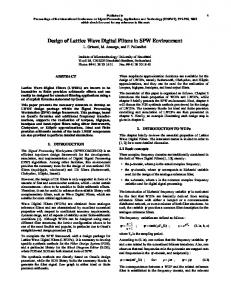
we extend the method of Fränken et al. [48,49]2 by making two observations. First, their method can be applied to circuits with multiport nonlinearities—to avoid splitting them up during the “split components” search, we apply their replacement graph technique to multiport nonlinear elements. Second, we note that designating all nonlinear elements (oneand multi-port) in a reference circuit as a collection which must not be separated, replacing it with a single replacement graph, and searching for split components yields an SPQR tree with all nonlinear elements embedded in a root element. Typically it is an R-type topology: a topology which cannot be decomposed further into series and parallel topologies. Rarely, it could have series or parallel topology [19]. In those cases, our method remains just as applicable—the root node should just be called S or P as appropriate. In all cases, the scattering at this topology can be found using a method derived from Modified Nodal Analysis (MNA) [55, 56], which is described in detail in a companion paper [47]. A WDF adaptor structure follows from the derived SPQR tree. This structure contains all of the nonlinear circuit elements embedded inside of a complicated R-type topology. All of the WDF subtrees that hang below this root collection may be handled with standard techniques. The behavior of the root element itself, however, is not entirely obvious at first. To decompose this problem into pieces that are more approachable, we propose a modification to the SPQR tree of Fränken et al.—this modification involves pulling all of the nonlinear circuit elements out of the root R-type adaptor and placing them above the R-type adaptor. Hence the vector nonlinearity is separated from the scattering. With both scattering and the nonlinear elements described in the wave domain, this problem framework is summarized by wave nonlinearity scattering

 a = f (bI ) ( I bI = S11 aI + S12 aE bE = S21 aI + S22 aE ,

(1) (2) (3)

with external incident and reflected wave vectors aE and bE , internal incident and reflected wave vectors aI and bI , scattering  11  S12 matrix S = S S21 S22 , and vector nonlinear function f (·). This is shown as a vector signal flow graph in Fig. 1a. 4. LOOP RESOLUTION There are two issues with (1)–(3) / Fig. 1a. First, they typically form an implicit and coupled set of transcendental equations— something that will not be convenient to solve. Second, there is a noncomputable delay-free loop through f (·) and S11 . This combination of an R-type scattering matrix and a vector of nonlinearities at the root can potentially be handled in various ways. In this paper, we propose a special case of the K-method, a technique for resolving implicit loops in nonlinear state space (NLSS) systems which is well-known in physical modeling [57–59], as a solution. Our main framework separates (1)–(3) / Fig. 1a into three phenomenon: scattering (S and its partitions) between wave variables at external (aE , bE ) and internal (aI , bI ) ports, conversion (C and its partitions) between internal wave (aC , bC ) and Kirchhoff (v C , iC ) variables, and a vector nonlinear Kirchhoff domain relationship h(·) between v C and iC . This problem framework is

DAFX-2

2A

review of their method is given in [47].

Proc. of the 18th Int. Conference on Digital Audio Effects (DAFx-15), Trondheim, Norway, Nov 30 - Dec 3, 2015

Kirchhoff nonlinearity h(·) vC C11 C12

wave nonlinearity

S22

aE

bE

...

aI S11

S12

S21

S22

aE

bE

...

...

g(·)

...

(a)

bIC v

a iCI F

E

M

aE

bE

...

(b)

N

... (c)

bI p E

aI iC F

N

M

aE

bE

...

no delay-free loop

S21

h(·) consolidated multiplies

S11

transformed nonlinearity

bC

bI

scattering matrix

aI

Kirchhoff nonlinearity

scattering matrix

bI

S12

C21

C22

aC

f (·)

w–K converter

iC

... (d)

Figure 1: Framework signal flow graphs: (a) A framework (1)–(3) entirely in the wave domain; (b) A framework with a Kirchhoff-domain vector nonlinearity (4)–(10) involving Kirchhoff nonlinearity h(·), w–K converter C, and scattering matrix S; (c) S and C partitions consolidated into NLSS (14) matrices E, F, M, and N; and (d) resolving the delay-free loop by transforming iC = h(v c ) into iC = g(p) according to (15)–(16). In (b)–(d), aE is supplied by and bE delivered to classical WDF subtrees below.

summarized by Kirchhoff nonlinearity w–K converter compatibility

 i = h (v C ) ( C v C = C11 iC + C12 aC

(4)

b = C21 iC + C22 aC ( C aC = bI

(6) (7)

aI = bC bI = S11 aI + S12 aE

(8) (9)

bE = S21 aI + S22 aE

(10)

( scattering

(5)

and shown as a vector signal flow graph in Fig. 1b. In this form, the structure is still noncomputable due to the presence of multiple delay-free loops. To ameliorate this, we consolidate the eight S and C partitions into four matrices E, F, M, and N. First consider (5) and (10) in matrix form,    vC C12 = bE 0

0 S21



  aC C11 + aI 0

0 S22



 iC , aE

(11)

and (6)–(9) in matrix form (eliminating bI and bC ), 

I −C22

−S11 I







aC 0 = aI C21

S12 0





iC . aE

(12)

Solving (12) for internal port wave vectors [aTC , aTI ]T yields    aC S HC21 = 11 aI HC21

S12 + S11 HC22 S12 HC22 S12



 iC , aE

(13)

where H = (I − C22 S11 )−1 . Plugging (13) into (11) and recalling (4) yields a consolidated version of (4)–(10),  E = C12 (I + S11 HC22 ) S12     iC = h (v C ) F = C12 S11 HC21 + C11 v C = EaE + FiC with  M = S21 HC22 S12 + S22    bE = MaE + NiC N = S21 HC21 , (14) which is shown as a vector signal flow graph in Fig. 1c. In this form, the structure is still noncomputable due to one remaining delay-free loop. But, since it is now in a standard NLSS form (albeit one without states), the K-method can be used to render it computable. This yields  E = C12 (I + S11 HC22 ) S12   iC = g (p) p = EaE with M = S21 HC22 S12 + S22   N = S21 HC21 , (15) bE = MaE + NiC where h(·) : v C → iC and g(·) : p → iC are related by      p I −K v C = . iC 0 I iC

(16)

In general the loop resolution matrix K (the namesake of the Kmethod) depends on the chosen discretization method [57]. With no dynamics, we simply have K = F from (14). The explicit framework (15) is shown as a vector signal flow graph in Fig. 1d. Since each entry in p is formed by different linear combination of voltages and currents, we can consider p to be a pseudo-wave variable, albeit one without an immediate physical interpretation [60]. The transformation (16) allows us to tabulate solutions to h(·), which is explicit and easy to tabulate, and transform it to g(·), a

DAFX-3

Proc. of the 18th Int. Conference on Digital Audio Effects (DAFx-15), Trondheim, Norway, Nov 30 - Dec 3, 2015 Table 1: Big Muff Pi Circuit Elements.

domain where it would be difficult to tabulate directly. The general framework for a reference circuit with multiple/multiport nonlinearities is hence rendered tractable.

element Vin R17 R18 , VCC R19 R20 R21 C5 C6 C12

5. DERIVING SYSTEM MATRICES (15)–(16) / Fig. 1d requires C and S matrices that characterize the system; we briefly review their derivations. C follows directly from the standard WDF voltage wave definition. Recalling (5)–(6) / Fig. 1b, C defines the relationship among the voltages v C , currents iC , incident waves aC , and reflected waves bC at the internal ports. Accordingly, the values of these matrices come from wave variable definitions. Rearranging the standard voltage wave definition [1, 61] yields aC = v C + RI iC b C = v C − R I iC | {z }

→

voltage wave definition

v C = aC − RI iC bC = aC − 2RI iC | {z }

element Is(d) VT Is αF αR

rearranged

S matrices are found using a method which leverages Modified Nodal Analysis on an equivalent circuit. Recalling (9)–(10) / Fig. 1b, S defines how incident waves aE and aI scatter to yield reflected waves bE and bI ; hence S is derived from the topology around the root. A derivation for S was first presented in [46]. We briefly review the derivation here—it is discussed in detail in a companion paper [47]. First, an instantaneous Thévenin port equivalent to the R-type topology (which may include multiport linear elements) is formed; each port n is replaced by a resistive voltage source with value an and resistance Rn (equal to the port resistance). This circuit is described by Modified Nodal Analysis as      Y A vn i = s , (19) B D j e | {z } MNA matrix X

where X partitions Y, A, B, and D are found by well-known element stamp procedures [55, 56, 58, 59]. Confronting (19) with wave variable definitions and compatibility requirements yields    T S = I + 2 0 R X−1 0 I , (20) where R = diag(RI , RE ) is a diagonal matrix of port resistances. S11 , S12 , S21 , and S22 are found simply by partitioning S. 6. CASE STUDY As a case study on the methods presented in this paper, we model the first clipping stage from the Big Muff Pi distortion pedal [62]. This circuit has three nonlinear elements: two 1N914 diodes (D3 and D4 ) and a 2N5089 BJT. We combine the two diodes into a single one-port nonlinearity as in [28, 29, 34, 35, 45]. Hence the WDF we derive has three nonlinear ports: the diode pair, the BJT’s VBE junction, and the BJT’s VCE junction. The names, values, and graph edges of each circuit element are shown in Table 1; coefficients pertaining to the nonlinear behavior of the diodes and transistor are shown in Table 2.

edge 1 5 9 3 4 8 2 7 6

Table 2: Big Muff Pi Circuit Elements.

(17)

where RI is a diagonal matrix of internal port resistances. Hence:     C11 C12 −RI I C= = . (18) C21 C22 −2RI I

value (input) V 470 kΩ 10 kΩ, 9 V 10 kΩ 100 kΩ 150 Ω 100 nF 470 pF 1 µF

value 2.52 nA 25.85 mV 5.911 fA 0.9993 0.5579

description diode reverse saturation current thermal voltage BJT reverse saturation current BJT forward current gain BJT reverse current gain

The derivation of a WDF from the Big Muff Pi clipping stage is shown in Fig. 2; details follow. The Big Muff Pi first clipping stage circuit is shown in Fig. 2a. Using the method of Fränken et al. [49], a connected graph structure is formed. In this graph (Fig. 2b), each circuit port corresponds to a graph edge, which is assigned an integer index. As described in §3, we extend the replacement graph approach of Fränken et al. to the nonlinear case—all nodes that are connected to a nonlinear element (nodes d, e, f , and g) are bundled together using a replacement graph, shown in gray in Fig. 2b. A standard search for split components yields the graph shown in Fig. 2e. As expected, the replacement graph has no splits and has ended up embedded in an R-type topology which cannot be decomposed further into series and parallel connections. We form a modified SPQR tree by designating the R-type topology as the root of a tree and letting the remaining one-ports and adaptors dangle below it (Fig. 2d). Here we break from standard technique, by extracting the three nonlinear ports (the diode pair D3,4 , VBC , and VBE , designated with a dark gray background) from the R-type adaptor and placing them above the root element (designated by a light gray background). A WDF tree (Fig. 2e) follows from the modified SPQR tree of Fig. 2d; a rearranged version of Fig. 2a which highlights the derived adaptor structure is shown in Fig. 2f. Note that Vin is given a fictitious 1 Ω source resistance to avoid having a non-root ideal voltage source, which would cause computability issues. Recall that a WDF adaptor can have only a single “reflectionfree port.” Since the R-type adaptor would need three reflectionfree ports to guaranteed realizability in the standard WDF framework, we make recourse to the techniques presented in §4 to handle the collection of the R-type adaptor and the nonlinearities. The rest of the adaptors and one-ports form WDF subtrees which are already computable with traditional techniques. The behavior of R and the nonlinearities is described by a system in the form of Fig. 1b. Here, w–K converter matrix C partitions are given by the vector form of standard voltage wave definitions (18). Scattering matrix S partitions describe the scattering behavior of the root R-type adaptor (Fig. 2g) and can be found using our MNA-derived method (20) on its instantaneous Thévenin port equivalent (Fig. 2h). Our matrix of port resistances

DAFX-4

Proc. of the 18th Int. Conference on Digital Audio Effects (DAFx-15), Trondheim, Norway, Nov 30 - Dec 3, 2015

c

C12

2 R18

C6

e

D3 2 c

b

d

− +

(a) Big Muff Pi clipping stage.

4

8

4

1

d

a

P2

a

(b) Graph structure.

D4

D4

C12

R18

R21

C6

R20

C12

R17

− +

R17 C5

2

aC

bC

aB

bB

bA

aA

iA

eH ...

aH

bD

R ...

...

...

9

...

RH

...

+ vA −

jH

...

iH +

eG 8

6

jA

RB

4

iB

+ vB −

eB jB

RC iC

+ vC −

1

11 12

10

jG

...

eA

13

− vH

bE

aE

aD

bF

aF

bG

aG

bH

3 − +

...

...

− +

...

C5

(f) Circuit arranged to highlight WDF structure.

RA ...

Vin

1Ω R19

4

...

R20

Vin

(e) Corresponding WDF adaptor structure.

...

S2

2 3 (d) Modified SPQR.

R18

1Ω R19

...

6

VCC − +

...

5

R21

VCC

2

a

(c) Finding split components. D3

R

1

8

10

D3

C6

30

g 9

R

10

S1

4

f

P1

7 8 9 20

d

20

g 9

R21

20

a

f

P2

7

−vG + iG − +

RG

jF eF

−vF + iF − +

RF

jE eE

−vE + iE − +

RE

8 7 6 (h) Instantaneous Thévenin port equivalent.

(g) R-type adaptor detail.

Figure 2: Deriving a WDF adaptor structure for the Big Muff Pi clipping stage.

DAFX-5

eC jC +i D

RD

jD

eD

vD −

− +

R20

3

e

d

R 40

10

− +

R19

Vin

S1

1

P1

40 40

d

30

7

Vout C5

b

VBE

3

30

5

VCC

D4

S2

b

6

D3,4 VBC d

− +

R17

6 5

f

5

Proc. of the 18th Int. Conference on Digital Audio Effects (DAFx-15), Trondheim, Norway, Nov 30 - Dec 3, 2015

2



2

3

4

5

6

7

8

9

10

11

12

GA

0

0

0

0

0

0

0

0

0

0

13

A

−GA 1

 0 0 0 0 0 0 0 0 0 0 0 3  GB  0 0 0 0 0 0 0 0 0 0 4  GC −GC  0 0 0 0 0 0 0 0 0 0 5  GD −GD  0 0 0 0 0 0 0 0 0 0 6  GE −GE  0 0 0 0 0 0 0 0 0 0 7  GF −GF  0 0 0 0 0 0 0 0 0 0 0 8  GG  0 0 0 0 0 0 0 0 0 0 9  GH −GH  0 0 0 0 0 0 0 0 0 10  −GC −GH GC + GH    Y A 0 0 0 0 0 0 0 0 0 0 −GD GD = 11  X=  B D 0 0 0 0 0 0 0 0 12  −GE −GF 0 GE + GF  0 0 0 0 0 0 0 0 0 0 13  −GA GA  0 0 0 0 0 0 0 0 0 0 0 A 1  0 0 0 0 0 0 0 0 0 0 B 1 −1  0 0 0 0 0 0 0 0 0 0 C 1 −1  0 0 0 0 0 0 0 0 0 0 D 1 −1  0 0 0 0 0 0 0 0 0 0 E 1 −1  0 0 0 0 0 0 0 0 0 0 0 F  1  0 0 0 0 0 0 0 0 0 0 G 1 −1 0 0 0 0 0 0 0 0 0 0 H 1 −1

0 0 0 0 0 0 0 0 0 0 0 0 0 0 0 0 0 0 0

B

C

D

E

F

G

H

0

0

0

0

0

0

0

1

0

0

0

0

0

0

0

1

0

0

0

0

0

0

0

0

0

0

0

0



    0 0 1 0 0 0 0   0 0 0 1 0 0 0    0 0 0 0 1 0 0   0 0 0 0 0 1 0   0 0 0 0 0 0 1   −1 0 0 −1 0 −1 0   0 0 0 0 0 0  −1  0 0 −1 0 0 0 0   0 0 0 0 0 0 −1   0 0 0 0 0 0 0   0 0 0 0 0 0 0   0 0 0 0 0 0 0    0 0 0 0 0 0 0   0 0 0 0 0 0 0  0 0 0 0 0 0 0   0 0 0 0 0 0 0 

Figure 3: Big Muff R-type adaptor MNA matrix—example resistor stamp in light shading, example voltage source stamp in dark shading.

is R = diag(RI , RE ), where RI = diag(RA , RB , RC ) and RE = diag(RD , RE , RF , RG , RH ) are matrices of internal and external port resistances. RE is prescribed by the port resistances of the WDF subtrees, and the port resistances in RI are assigned arbitrarily as RA = RB = RC = 1 kΩ; we cannot make all three internal ports reflection-free, and they will get resolved by the K-method anyways, so we don’t even try to adapt any of them. The MNA system matrix X that arises from the stamp procedure, with node 1 as the datum node, is shown in Fig. 3. The behavior of our vector of nonlinearities is described in the Kirchhoff domain by h(·), which maps a vector of voltages v C = [vdiodes , vBC , vBE ]T to a vector of currents iC = [idiodes , −iC , iE ]T according to the Shockley ideal diode law, idiodes = Is(d) (evdiodes /VT − 1) − Is(d) (e−vdiodes /VT − 1) , (21) and the Ebers–Moll BJT model, iC = Is (eVBE /VT − 1) − Is /αR (eVBC /VT − 1) VBE /VT

iE = Is /αF (e

VBC /VT

− 1) − Is (e

− 1) .

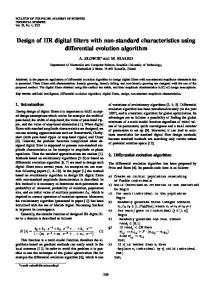
time step during runtime, these subtrees deliver a length-5 vector of incident waves aE = [aD , aE , aF , aG , aH ]T to R. We find length-3 vector p from aE by p = EaE . Using scattered interpolant methods3 , we find length-3 vector iC from p by iC = g(p). Finally the length-5 output vector bE of the root R–nonlinearity collection is found by combining contributions from aE and iC by bE = MaE + Ni. bE is propagated down into the standard WDF subtrees and we can advance to the next time step. Simulation results are shown in Fig. 4. On top is a 15-ms-long guitar input signal Vin . The middle panel compares a “groundtruth” SPICE simulation and the results of our WDF algorithm. They are nearly a match, confirming the validity of our novel WDF formulation. The error signal between the two is shown in the bottom panel; small discrepancies can be ascribed to limitations of the 201×201×201 lookup table, (expected) aliasing in the WDF, linear resampling of the SPICE output to WDF simulation’s constant time grid for comparison, and general numerical concerns.

(22) (23)

h(·) is tabulated with a 201×201×201 grid across the circuit’s operating range of voltages (determined experimentally with SPICE). Since this structure contains multiple noncomputable loops, it is collapsed down into a NLSS form (Fig. 1c), where the values of E, F, M, and N are given as functions of C11 , C12 , C21 , C22 , S11 , S12 , S21 , and S22 by (14). This structure still contains a noncomputable loop through h(·) and F, but since it is a standard NLSS system (albeit one without states), we can render it computable using the K-method [57–59], yielding a system in the form of Fig. 1d / (15). Matrices E, M, and N are already known, and a scattered tabulation g(·) is found from the gridded tabulation h(·), using K = F according to (16). To explain how the system is computable, let us walk through one time step of the algorithm. All of the WDF subtrees which dangle from R are handled in the normal way, and the collection of R and the nonlinearities are handled according to (15). At each

7. CONCLUSION AND FUTURE WORK In this paper, we’ve presented a framework for modeling lumped systems (in particular, electronic circuits) with multiple and multiport nonlinear elements and arbitrary topologies as Wave Digital Filters. We expand on the graph-theoretic approach of Fränken et al. [48, 49], applying it rather to yield an adaptor structure for circuits with multiple/multiport nonlinearities. Replacing the collection of all nonlinear elements with a single replacement graph during the separation-pair-finding process yields a modified SPQR tree, where the root node tends to be an R-type adaptor, with standard WDF subtrees hanging below and a vector of nonlinearities hanging above. This confines issues of computability to a minimal subsytem comprised of the R-type adaptor and vector of nonlinearities at the root of a WDF tree. 3 http://www.mathworks.com/help/matlab/ref/ scatteredinterpolant-class.html

DAFX-6

Proc. of the 18th Int. Conference on Digital Audio Effects (DAFx-15), Trondheim, Norway, Nov 30 - Dec 3, 2015

Vin (volts)

0.1 0.05 0 −0.05 −0.1 5

6

7

8

9

10

11

12

13

14

15

16

17

Vout (volts)

4.4

18

19

20

SPICE WDF

4.3 4.2

Vout error (mV)

4.1 5

6

7

8

9

10

11

12

13

14

15

16

17

18

19

20

5

6

7

8

9

10

11 12 13 14 15 time (milliseconds)

16

17

18

19

20

5 2.5 0 −2.5 −5

Figure 4: Big Muff Pi clipping stage simulation. Vin (top), Vout from SPICE and WDF (middle), and WDF Vout error (bottom). SPICE used a maximum time step of 10−5 seconds and WDF simulation used a sampling rate of 44.1 kHz.

This combination of this R-type adaptor and the vector of nonlinearities is noncomputable. To render it computable, we rearrange it so our system of “consolidated multiplies” E, F, M, and N is solvable with the K-method [57–59]. The advantage of solving the root collection with the K-method is that tabulation can be done simply in the Kirchhoff domain, where iC –v C relationships are usually explicit and memoryless.4 A disadvantage is that when gridded tabulation is transformed to the p–iC domain, it will no longer be gridded, limiting interpolation to scattered methods. We’ve focused on creating a general problem framework with the potential for solution through diverse methods, not only the K-method-derived approach we’ve proposed. Future work should investigate computational efficiency and other methods for solving the localized minimal root subsystem. The internal structure of S, C, E, F, M, and N could potentially be exploited for computational saving in future work. Using iterative techniques to tabulate the p–iC domain directly, rather than transforming an iC –v C tabulation, it should be possible to create a gridded tabulation, opening up the possibility of using gridded interpolant methods. This would require good initial guesses for the iterative solver or the use of, e.g., Newton Homotopy [58, 59]. Potentially, a transformed solution could be used as initial guesses for forming a gridded interpolation [34]. We could consider keeping our root topology R and vector of nonlinearities entirely in the wave domain, as in Fig. 1a. In this case, a nonlinear wave-domain function f (·) would need to solve aI = f (bI ). This system could also be resolved with the K-method. However, it is unlikely that a closed-form solution to f (·) will be available, so an explicit solution can’t be tabulated for 4 Nonlinearities “with memory,” e.g., NL inductors/capacitors, can be expressed as instantaneous aspects combined with WDF “mutators” [11].

f (·) and then transformed. With iterative techniques, tabulation in the transformed f (·) domain should be possible. As another option, the instantaneous Thévenin port equivalent concept could be applied to all external ports of the nonlinear root node topology and vector nonlinearity, creating a Kirchhoffdomain subsystem grafted onto standard WDF subtrees below. As in the scattering matrix derivation [47], each external port n in the root scattering matrix would be replaced by its instantaneous Thévenin equivalent—a series combination of a voltage source with a value equal to the incident wave an and a resistor equal to the port resistance Rn —and then the system could be solved with the K-method or any other Kirchhoff-domain method. In our main formulation or the others proposed above, one could develop alternate derivations that exchange the roles of currents and voltages, using e.g., v C = g −1 (iC ). This may be particularly applicable to using iterative methods to tabulate the nonlinearities; Yeh et al. report that iteration on terminal voltages converges faster than iteration on device currents [58]. Future work should explore these alternate formulations and practical aspects of N -dimensional scattered interpolation. Our exposition uses standard voltage wave variables for simplicity of presentation, but for time-varying structures, power waves provide theoretical energetic advantages [15, 61, 63]. For alternative wave variable definitions, (17)–(18) will be modified as appropriate. Energetic concerns in the root subsystem remain unexplored and potentially problematic, e.g., for highly resonant circuits. Previous work investigates energetic aspects of nonlinear table interpolation techniques in WDFs [41]—although it is limited to the one-port case, it could serve as a prototype for future work. 8. REFERENCES [1] A. Fettweis, “Wave digital filters: Theory and practice,” Proc. IEEE, vol. 74, no. 2, pp. 270–327, 1986. [2] J. O. Smith III, Physical Audio Signal Processing for Virtual Musical Instruments and Audio Effects, online book, 2010 edition. [3] V. Välimäki et al., “Introduction to the special issue on virtual analog audio effects and musical instruments,” IEEE Trans Audio, Speech, Language Process., vol. 18, no. 4, pp. 713–714, 2010. [4] V. Välimäki et al., Virtual Analog Effects, chapter 12, pp. 473–522, John Wiley & Sons, second edition, 2011, Appears in [64]. [5] V. Välimäki, “Virtual analog modeling,” in Int. Conf. Digital Audio Effects (DAFx-13), Maynooth, Ireland, Sept. 5 2013, keynote. [6] E. Barbour, “The cool sound of tubes,” IEEE Spectr., vol. 35, no. 8, pp. 24–35, Aug. 1998. [7] K. Meerkötter and R. Scholz, “Digital simulation of nonlinear circuits by wave digital filter principles,” in Proc. IEEE Int. Symp. Circuits Syst., June 1989, vol. 1, pp. 720–723. [8] T. Felderhoff, “Simulation of nonlinear circuits with period doubling and chaotic behavior by wave digital filter principles,” IEEE Trans. Circuits Syst. I: Fundam. Theory Appl., vol. 41, no. 7, 1994. [9] T. Felderhoff, “A new wave description for nonlinear elements,” in Proc. IEEE Int. Symp. Circuits Syst., Sept. 1996, vol. 3, pp. 221–224. [10] A. Sarti and G. De Poli, “Generalized adaptors with memory for nonlinear wave digital structures,” in Proc. European Signal Process. Conf. (EUSIPCO), Sept. 1996, vol. 3, pp. 1941–1944. [11] A. Sarti and G. De Poli, “Toward nonlinear wave digital filters,” IEEE Trans. Signal Process., vol. 47, no. 6, pp. 1654–1668, 1999. [12] F. Pedersini et al., “Block-wise physical model synthesis for musical acoustics,” Electron. Lett., vol. 35, no. 17, pp. 1418–1419, 1999. [13] F. Pedersini et al., “Object-based sound synthesis for virtual environments using musical acoustics,” IEEE Signal Process. Mag., vol. 17, no. 6, pp. 37–51, Nov. 2000. [14] G. De Sanctis, “Una nuova metodologia per l’implementazione automatica di strutture ad onda numerica orientata alla modellazione ad oggetti di interazioni acustiche,” M.S. thesis, Politecnico di Milano, Italy, 2002.

DAFX-7

Proc. of the 18th Int. Conference on Digital Audio Effects (DAFx-15), Trondheim, Norway, Nov 30 - Dec 3, 2015

[15] S. Bilbao et al., “A power-normalized wave digital piano hammer,” in Proc. Meeting Acoust. Soc. Amer., Cancun, Mexico, 2002, vol. 114. [16] S. Bilbao et al., “The wave digital reed: A passive formulation,” in Proc. Int. Conf. Digital Audio Effects (DAFx-03), London, UK, Sept. 8–11 2003, vol. 6, pp. 225–230. [17] M. Karjalainen, “BlockCompiler: Efficient simulation of acoustic and audio systems,” in Proc. Audio Eng. Soc. (AES) Conv., Amsterdam, The Netherlands, Mar. 22–25 2003, vol. 114. [18] G. De Sanctis et al., “Automatic synthesis strategies for object-based dynamical physical models in musical acoustics,” in Proc. Int. Conf. Digital Audio Effects, London, UK, Sept. 8–11 2003, vol. 6. [19] S. Petrausch and R. Rabenstein, “Wave digital filters with multiple nonlinearities,” in Proc. European Signal Process. Conf. (EUSIPCO), Vienna, Austria, Sept. 2004, vol. 12. [20] M. Karjalainen, “Efficient realization of wave digital components for physical modeling and sound synthesis,” IEEE Trans. Audio, Speech, Language Process., vol. 16, no. 5, pp. 947–956, 2008. [21] M. Karjalainen and J. Pakarinen, “Wave digital simulation of a vacuum-tube amplifier,” in Proc. IEEE Int. Conf. Acoust., Speech, Signal Process., Toulouse, France, May 14–19 2006, pp. 153–156. [22] J. Pakarinen et al., “Wave digital modeling of the output chain of a vacuum-tube amplifier,” in Proc. Int Conf. Digital Audio Effects (DAFx-09), Como, Italy, Sept. 1–4 2009, pp. 153–156. [23] J. Pakarinen and M. Karjalainen, “Enhanced wave digital triode model for real-time tube amplifier emulation,” IEEE Trans. Audio, Speech, Language Process., vol. 18, no. 4, pp. 738–746, 2010. [24] S. Petrausch, Block based physical modeling, Ph.D. diss., FriedrichAlexander-Universität Erlangen–Nürnberg, Germany, 2006. [25] R. Rabenstein et al., “Block-based physical modeling for digital sound synthesis,” IEEE Signal Process. Mag., pp. 42–54, Mar. 2007. [26] R. Rabenstein and S. Petrausch, “Block-based physical modeling with applications in musical acoustics,” Int. J. Appl. Math. Comput. Sci., vol. 18, no. 3, pp. 295–305, 2008. [27] D. T.-M. Yeh, “Tutorial on wave digital filters,” https://ccrma. stanford.edu/~dtyeh/papers/wdftutorial.pdf, Jan. 25 2008. [28] D. T.-M. Yeh and J. O. Smith III, “Simulating guitar distortion circuits using wave digital and nonlinear state-space formulations,” in Proc. Int. Conf. Digital Audio Effects (DAFx-08), Espoo, Finland, Sept. 1–4 2008, vol. 11, pp. 19–26. [29] D. T.-M. Yeh, Digital implementation of musical distortion circuits by analysis and simulation, Ph.D. diss., Stanford Univ., CA, 2009. [30] A. Sarti and G. De Sanctis, “Systematic methods for the implementation of nonlinear wave-digital structures,” IEEE Trans. Circuits Syst. I: Reg. Papers, vol. 56, no. 2, pp. 460–472, 2009. [31] G. De Sanctis and A. Sarti, “Virtual analog modeling in the wavedigital domain,” IEEE Trans. Audio, Speech, Language Process., vol. 18, no. 4, pp. 715–727, 2010. [32] R. C. D. de Paiva et al., “Real-time audio transformer emulation for virtual tube amplifiers,” EURASIP J. Adv. Signal Process., 2011. [33] P. Raffensperger, “Toward a wave digital filter model of the Fairchild 670 limiter,” in Proc. Int. Conf. Digital Audio Effects (DAFx-12), York, UK, Sept. 17–21 2012, vol. 15. [34] R. C. D. Paiva et al., “Emulation of operational amplifiers and diodes in audio distortion circuits,” IEEE Trans. Circuits Syst. II: Exp. Briefs, vol. 59, no. 10, pp. 688–692, 2012. [35] R. C. D. de Paiva, Circuit modeling studies related to guitars and audio processing, Ph.D. diss., Aalto Univ., Espoo, Finland, 2013. [36] S. D’Angelo and V. Välimäki, “Wave-digital polarity and current inverters and their application to virtual analog audio processing,” in Proc. IEEE Int. Conf. Acoust., Speech, Signal Process. (ICASSP), Kyoto, Japan, Mar. 2012, pp. 469–472. [37] S. D’Angelo et al., “New family of wave-digital triode models,” IEEE Trans. Audio, Speech, Language Process., vol. 21, no. 2, pp. 313–321, 2013. [38] S. D’Angelo, Virtual Analog Modeling of Nonlinear Musical Circuits, Ph.D. diss., Aalto University, Espoo, Finland, Sept. 2014. [39] T. Schwerdtfeger and A. Kummert, “A multidimensional signal processing approach to wave digital filters with topology-related delayfree loops,” in Proc. IEEE Int. Conf. Acoust., Speech, Signal Process. (ICASSP), Florence, Italy, May 4–9 2014, pp. 389–393.

[40] T. Schwerdtfeger and A. Kummert, “A multidimensional approach to wave digital filters with multiple nonlinearities,” in Proc. European Signal Process. Conf. (EUSIPCO), Lisbon, Portugal, Sept. 1–5 2014. [41] K. J. Werner and J. O. Smith III, “An energetic interpretation of nonlinear wave digital filter lookup table error,” in Proc. IEEE Int. Symp. Signals, Circuits, Syst. (ISSCS), Ias, i, Romania, July 9–10 2015. [42] A. Bernardini et al., “Multi-port nonlinearities in wave digital structures,” in Proc. IEEE Int. Symp. Signals, Circuits, Syst. (ISSCS), Ias, i, Romania, July 9–10 2015. [43] A. Bernardini et al., “Modeling a class of multi-port nonlinearities in wave digital structures,” in Proc. European Signal Process. Conf. (EUSIPCO), Nice, France, Aug. 31 – Sept. 4 2015, vol. 23. [44] A. Bernardini, “Modeling nonlinear circuits with multiport elements in the wave digital domain,” M.S. thesis, Politecnico di Milano, Italy, Apr. 2015. [45] K. J. Werner et al., “An improved and general diode clipper model for wave digital filters,” in Proc. Audio Eng. Soc. (AES) Conv., New York, NY, Oct. 29 – Nov. 1 2015, vol. 139. [46] K. J. Werner et al., “A general and explicit formulation for wave digital filters with multiple/multiport nonlinearities and complicated topologies,” in Proc. IEEE Workshop Appl. Signal Process. Audio Acoust. (WASPAA), New Paltz, NY, Oct. 18–21 2015. [47] K. J. Werner et al., “Wave digital filter adaptors for arbitrary topologies and multiport linear elements,” in Proc. Int. Conf. Digital Audio Effects, Trondheim, Norway, Nov. 30 – Dec. 3 2015, vol. 18. [48] D. Fränken et al., “Generation of wave digital structures for connection networks containing ideal transformers,” in Proc. Int. Symp. Circuits Systems (ISCAS), May 25–28 2003, vol. 3, pp. 240–243. [49] D. Fränken et al., “Generation of wave digital structures for networks containing multiport elements,” IEEE Trans. Circuits Systems I: Reg. Papers, vol. 52, no. 3, pp. 586–596, Mar. 2005. [50] A. Fettweis, “Some principles of designing digital filters imitating classical filter structures,” IEEE Trans. Circuit Theory, vol. 18, no. 2, pp. 314–316, 1971. [51] A. Fettweis, “Digital filters structures related to classical filter networks,” Archiv Elektronik Übertragungstechnik (AEÜ, Int. J. Electron. Commun.), vol. 25, pp. 79–89, 1971. [52] A. Fettweis, “Pseudo-passivity, sensitivity, and stability of wave digital filters,” IEEE Trans. Circuit Theory, vol. 19, no. 6, 1972. [53] A. Fettweis, “Reciprocity, inter-reciprocity, and transposition in wave digital filters,” Int. J. Circuit Theory Appl., vol. 1, no. 4, pp. 323–337, Dec. 1973. [54] A. Fettweis and K. Meerkötter, “On adaptors for wave digital filters,” IEEE Trans. Acoust., Speech, Signal Process., vol. 23, no. 6, 1975. [55] C.-W. Ho et al., “The modified nodal approach to network analysis,” IEEE Trans. Circuits Systems, vol. 22, no. 6, pp. 504–509, 1975. [56] J. Vlach and K. Singhal, Computer methods for circuit analysis and design, Springer, 1983. [57] G. Borin et al., “Elimination of delay-free loops in discrete-time models of nonlinear acoustic systems,” IEEE Trans. Speech Audio Process., vol. 8, no. 5, pp. 597–605, 2000. [58] D. T.-M. Yeh et al., “Automated physical modeling of nonlinear audio circuits for real-time audio effects—part I: Theoretical development,” IEEE Trans. Audio, Speech, Language Process., vol. 18, no. 4, pp. 728–737, 2010. [59] D. T.-M. Yeh, “Automated physical modeling of nonlinear audio circuits for real-time audio effects—part II: BJT and vacuum tube examples,” IEEE Trans. Audio, Speech, Language Process., vol. 20, no. 4, pp. 1207–1216, 2012. [60] S. S. Lawson, “On a generalization of the wave digital filter concept,” Int. J. Circuit Theory Appl., vol. 6, no. 2, pp. 107–120, 1978. [61] S. Bilbao, Wave and Scattering Methods for Numerical Simulation, John Wiley & Sons, New York, July 2004. [62] Electrosmash, “Bi Muff Pi analysis,” http://www. electrosmash.com/big-muff-pi-analysis. [63] G. Kubin, “Wave digital filters: Voltage, current, or power waves?,” in Proc. IEEE Int. Conf. Acoust., Speech, Signal Process. (ICASSP), Tampa, FL, Apr. 1985, vol. 10, pp. 69–72. [64] U. Zölzer, Ed., DAFX: Digital Audio Effects, John Wiley & Sons, second edition, 2011.

DAFX-8