Resource-Constrained Multi-Project Management

Resource -Constrained Multi -Project Management - A Hierarchical Decision Support System -

Ronald de Boer

ISBN 90-36512069 c 1998, Ronald de Boer ° Printed by Febodruk B.V., Enschede, The Netherlands

RESOURCE -CONSTRAINED MULTI-PROJECT MANAGEMENT - A HIERARCHICAL DECISION SUPPORT SYSTEM -

PROEFSCHRIFT

ter verkrijging van de graad van doctor aan de Universiteit Twente, op gezag van de Rector Magni…cus, prof.dr. F.A. van Vught, volgens besluit van het College voor Promoties in het openbaar te verdedigen op vrijdag 6 november 1998 te 16.45 uur.

door

Ronald de Boer geboren op 26 april 1970 te Nunspeet

Dit proefschrift is goedgekeurd door de promotoren: prof.dr. W.H.M. Zijm prof.dr. A. van Harten

To Marjan and Anne

To choose time is to save time F. Bacon

ii

iii

Preface The research presented in this thesis was primarily inspired by a practical situation at the Royal Netherlands Navy (RNN) Dockyard. The management of this organization has to coordinate a large set of orders, with much variety in size and complexity, subject to various restrictions, such as precedence relations and resource constraints. Quoting tight due dates and meeting them within shrinking budgets is a very complex task that requires a ‡exible organization and a sophisticated information system. This research focused on the latter. Since production planning software, including many project management information systems, do not o¤er the support required in this environment, the job was to design a new decision support system and actually build it. A very fascinating aspect of this research is that it addresses practical problems that are hard to solve from a mathematical point of view. Communicating about these problems and possible solutions with practice-oriented people that have little knowledge of scheduling theory was therefore a big challenge. Although the prototyping approach we followed required a lot of time and energy, it appeared to be extremely valuable in facilitating this communication process. When people started working with a premature version of the prototype DSS, they were able to esteem the added value of such a system and to contribute to the design. Another side-e¤ect was that it urged the RNN dockyard to reconsider which factors comprise real constraints and what primary objectives should be selected. In April 1994 I was o¤ered a PhD.-position at the University of Twente. I still remember the day that Henk Zijm phoned me to say that I could start

iv

Preface

with the ‘Navy project’. At …rst, I thought he was mistaken since I had applied for another PhD.-project, that was also o¤ered by him and Aart van Harten. I even did not know there was a ‘Navy project’. Nevertheless, after some more inspiring explanation of Henk, I decided to accept the o¤er. Looking back, I can say that this project was exactly what I was looking for. In the …rst place, it gave me the opportunity to become more acquainted with the …eld of production and operations management. Next, there were many opportunities to visit a number of national and international project-driven organizations and …nd out what problems they face. In addition, I had (relatively) much time to design, implement, and evaluate planning and scheduling solutions. Finally, I really appreciated the fact that my research resulted in a real ‘product’. One of the most important lessons for me was to see how much e¤ort it costs to build a DSS and subsequently make people work with it, but also how satisfactory it can be. Many people contributed to my work in various ways. In the …rst place, I want to thank Henk Zijm and Aart van Harten. My project was based on a joint research proposal by the Faculty of Mechanical Engineering (ME) and the Faculty of Technology & Management (T&M) at the University of Twente. Consequently, I worked for both the Production and Operations Management (POM) Group of Henk Zijm (ME) as well as the Operational Methods and Systems Theory (OMST) Group of Aart van Harten (T&M). Although this meant that the principle of unity of command was sacri…ced (cf. Chapter 2 of this thesis) and induced some practical problems, they were creative enough to …nd (near) optimal solutions. I am thankful for their precious time and their useful ideas and observations. Besides, I appreciate their willingness to support good initiatives and to provide the necessary tools. Next, there is a large group of people at the RNN Dockyard who made this research possible. First, I thank Commodore RNLN W.M. van Gulpen and Captain RNLN B. Wienbelt who initiated this project, as well as Captain RNLN W.A. Dekker, who continued to support it. Furthermore, I appreciate the assistance and useful comments of the steering group, the project group, and the user group. Arie-Jan de Waard, who started about the same time as I, did his PhD research on restructuring large-scale maintenance organizations

Preface

v

at the RNN Dockyard. He spent much time to introduce me to the Dockyard organization, for which I am grateful. Two years later, Jan-Willem Rustenburg started his research on materials coordination and spare part management at the Dockyard. As a team, we had many discussions about the project, prepared joint presentations, and visited various companies. To me, these moments were very valuable and pleasant. In addition, I thank Daan Meijer, Joop van Vliet, Wim Rossen, Roel Engeltjes, and Marco Groenestein, who spent much time to facilitate the testing and analyzing of the prototype DSS. Next, Iam very grateful to my colleague Marco Schutten, who coached my research for the last two years and developed part of the prototype DSS. He was always there to advise me, showed me the art of implementing complex algorithms and data structures, and was great company on many of my trips. In the last four-and-a-half year, I had several room mates whose presence I appreciated very much. Gerhard van Dijkhuizen showed me how every problem in life may be translated into an Operations Research problem, while the discussions I had with Ronald Buitenhek always reminded me that life is much more than just work. Since the beginning of this year, Jan-Willem Rustenburg was my room mate. He gave me more insight in the Naval tradition and vocabulary. Besides, I thank all other members of the OMST group and the POM group. They created a pleasant and inspiring working atmosphere. Last, but not least, I like to thank my family and friends. In particular, I am grateful to my wonderful wife Marjan. She gave me all the love and encouragement I needed and shared in the ‘birth pains’ of realizing this thesis. Finally, I thank Anne, whose presence brought much joy.

Ronald de Boer Enschede, October, 1998

vi

Preface

vii

Summary Many industrial organizations exploit a project structure to cope with large and highly complex tasks. These tasks usually involve expertise from many different departments or groups, such as engineering, various production departments, process and production planning, and service. In such (semi-)projectdriven organizations, multiple projects compete for shared resources, such as manpower, machines, equipment, and space. The capacity of these resources is usually constrained on the short term or can only be increased at extra costs. At the same time, speed has become an essential competitive weapon: customers require short and reliable lead times. This leaves management of (semi-)project organizations with a very complex task: to quote tight, yet reliable delivery dates at a lowest possible cost and, next, to actually realize these goals. In this thesis, we argue that commercial production planning software does not provide su¢cient support for this complex task. This is not surprising since project management theory covers mostly isolated theoretical problems and does not o¤er a coherent framework for hierarchical planning in this type of organizations. The objective of the research presented in this thesis is the design of a decision support system (DSS) that can assist management of resource-constrained (semi-)project-driven organizations in planning and scheduling decisions. The philosophy behind the DSS is that it must be based on a hierarchical planning framework, since constraints and available data usually vary over time. Moreover, optimization techniques are employed in order to generate good-quality plans and schedules, while taking into account the major constraints that occur in practical situations.

viii

Summary

One of the characteristics of a project is that it has almost always unique elements, if not unique at all. This means that (semi-)project-driven organizations often face tasks that, at least initially, are characterized by a high uncertainty. Organizations may implement several strategies to cope with this uncertainty. In this thesis, we concentrate on organizations that deal with selfcontained activities and have a matrix structure and a portfolio management team. Self-contained activities are relatively large tasks that can be performed by a multi-disciplinary team, such that much of the coordination is delegated to the team itself. A matrix structure avoids to choose one prevailing basis for grouping. Instead, it structures an organization along several dimensions. In this case, the structure is based upon projects on the one hand and functional departments on the other. In a matrix organization, a portfolio management team, may be introduced to solve problems that arise as a result of interference between di¤erent orders. Basically, such a portfolio management team consits of project managers and managers of functional departments, who meet regularly to match the supply and demand of capacity. The purpose of the DSS is to assist the portfolio management team with major planning decisions, such as order acceptance (quoting reliable due dates, taking into account required and available capacity), priority setting (assigning internal due dates to activities), capacity management (deciding which type of non-regular capacity should be employed, and how much), material and capacity scheduling (allocating resources to activities over time), and crisis management (deciding how to respond to major disruptions, such as a rush order or a machine break-down). Within the DSS, we distinguish two planning levels: rough-cut capacity planning and resource-constrained project scheduling. Rough-cut capacity planning (RCCP) is used during order acceptance. Since a new project is likely to have unique elements, detailed information regarding precedence constraints and capacity and materials requirements may not be available. Therefore, it is more appropriate to use aggregate data, i.e., rough estimates of required resources and critical items, at this stage. New information will become available after engineering and process planning, resulting in a more detailed activity network, which is input for resource-constrained project sched-

Summary

ix

uling (RCPS). Not only the type of data required for both levels di¤er, but also the type of constraints: Since the RCCP has a longer planning horizon, it is easier to employ extra resource capacity. At the RCPS, on the other hand, capacity levels are, more or less, given. If possible at all, management may only be able to increase capacity for certain resources, at a relatively high cost. In order to deal with RCPS in (semi-)project-driven organizations, we propose a number of practical extensions to the standard RCPS problem, as it often occurs in literature. These extensions include: release and due dates, multiple execution modes, variable capacity pro…les, minimum time lags, and spatial resources. We introduce a heuristic, based on the adaptive search method of Kolisch and Drexl [45], that is able to deal with these extensions. We show that this heuristic is able to generate schedules that are signi…cantly better than those generated by priority rule based single-pass heuristics, while requiring only modest computation times. For the RCCP level, we distinguish the resource driven problem and the time driven problem. In the resource driven problem, we assume that capacity levels are …xed and cannot be exceeded, while the objective is to minimize the maximum lateness. In the time driven problem, on the other hand, we suppose that each project has a deadline that may not be exceeded and the objective is to minimize the sum of non-regular capacity used. We present a single-pass heuristic for the time driven problem, called ICPA, that, after some adaptations, can also be used for the resource driven problem. Moreover, we introduce a heuristic for the time driven problem that is based on an LP formulation. We show that the latter performs better than ICPA, but requires more computation time. A interactive prototype of the DSS has actually been built. In this prototype, the algorithms for both RCCP and RCPS are implemented. In order to perform what-if analyses, di¤erent input scenarios for these algorithms can be stored in a local database. In addition, the prototype has a user friendly graphical interface o¤ering data manipulation tools and a convenient plan board. Moreover, it o¤ers various schedule editing, analysis, and evaluation functions that enable the portfolio management team to get insight in the schedule performance, suggest alternatives, and evaluate them immediately.

x

Summary

The development of the prototype DSS was part of an organization wide reengineering project at the Royal Netherlands Navy Dockyard. We outline the major changes proposed by the reengineering project team and present a possible information architecture for the speci…c case of the Dockyard. Finally, we report on the experiences with the prototype DSS by a group of potential users. This group concludes that the system is very easy to use and that it generates realistic, high quality solutions in little time. Indeed, a DSS, as described in this thesis, may support the management of the Dockyard to make better planning decisions and hence to improve e¢ciency, ‡exibility, and due date performance signi…cantly.

xi

Contents Preface

iii

Summary

vii

1 Introduction 1.1 De…ning a Project . . . . . . . . . . . . . . . . . . . . . . . . . 1.2 Applications and Use of Project Management . . . . . . . . . . 1.3 Shifting Objectives . . . . . . . . . . . . . . . . . . . . . . . . . 1.4 The Project Life Cycle . . . . . . . . . . . . . . . . . . . . . . . 1.5 Project Management Theory - An Organizational Approach . . 1.5.1 Project Organization . . . . . . . . . . . . . . . . . . . . 1.5.2 Top-down Planning . . . . . . . . . . . . . . . . . . . . 1.6 Project Management Theory - A Quantitative Approach . . . . 1.6.1 Project Network Techniques . . . . . . . . . . . . . . . . 1.6.2 The Resource-Constrained Project Scheduling Problem 1.7 Project Management Software . . . . . . . . . . . . . . . . . . . 1.8 Project Management in Practice . . . . . . . . . . . . . . . . . 1.8.1 Surveys of Projects in Diverse Industries . . . . . . . . . 1.8.2 Project-Based Management at the Royal Netherlands Navy Dockyard . . . . . . . . . . . . . . . . . . . . . . . 1.9 A Decision Support System for Multi-Project Management . . 1.10 Overview of the Thesis . . . . . . . . . . . . . . . . . . . . . . .

1 2 4 6 8 10 10 11 13 13 17 20 21 22 23 25 26

xii

Contents

2 A Framework for Hierarchical Planning in (Semi-)ProjectDriven Organizations 2.1 Introduction . . . . . . . . . . . . . . . . . . . . . . . . . . . . . 2.2 Coordination Mechanisms for Complex Organizations . . . . . 2.3 The Matrix Structure and the Portfolio Management Team . . 2.4 A Framework for Hierarchical Planning . . . . . . . . . . . . . 2.5 Coordination at Each Project Stage . . . . . . . . . . . . . . . 2.5.1 Order Acceptance . . . . . . . . . . . . . . . . . . . . . 2.5.2 Engineering and Process Planning . . . . . . . . . . . . 2.5.3 Material and Resource Scheduling . . . . . . . . . . . . 2.5.4 Project Execution . . . . . . . . . . . . . . . . . . . . . 2.5.5 Evaluation & Service . . . . . . . . . . . . . . . . . . . . 2.6 Conclusions . . . . . . . . . . . . . . . . . . . . . . . . . . . . .

27 27 27 32 35 38 39 40 41 42 43 44

3 Resource-Constrained Project Scheduling 3.1 Introduction . . . . . . . . . . . . . . . . . 3.2 The Standard RCPSP . . . . . . . . . . . 3.3 A Classi…cation Scheme . . . . . . . . . . 3.4 Lower Bounds . . . . . . . . . . . . . . . . 3.5 Literature Review . . . . . . . . . . . . . 3.6 Priority-Rule-Based Scheduling . . . . . . 3.6.1 Schedule Generation Schemes . . . 3.6.2 Schedule Types . . . . . . . . . . . 3.6.3 Priority Rules . . . . . . . . . . . . 3.6.4 Sampling Procedures . . . . . . . . 3.7 Conclusions . . . . . . . . . . . . . . . . .

. . . . . . . . . . .

. . . . . . . . . . .

. . . . . . . . . . .

. . . . . . . . . . .

45 45 46 47 50 52 55 55 57 60 64 67

4 Practical Extensions to Resource-Constrained Project Scheduling 4.1 Introduction . . . . . . . . . . . . . . . . . . . . . . . . . . 4.1.1 Multiple Projects and Release and Due dates . . . 4.1.2 Minimum Time Lags . . . . . . . . . . . . . . . . . 4.1.3 Time Varying Capacity Pro…les . . . . . . . . . . . 4.1.4 Multiple Execution Modes . . . . . . . . . . . . . .

. . . . .

. . . . .

. . . . .

69 69 70 72 73 74

. . . . . . . . . . .

. . . . . . . . . . .

. . . . . . . . . . .

. . . . . . . . . . .

. . . . . . . . . . .

. . . . . . . . . . .

. . . . . . . . . . .

. . . . . . . . . . .

Contents

xiii

4.1.5 Spatial resources . . . . . . . . . 4.2 A New Heuristic . . . . . . . . . . . . . 4.2.1 Schedule Generation Schemes . . 4.2.2 Priority Rule and Mode Selection 4.2.3 Multi-Pass Sampling . . . . . . . 4.3 Instance Generation . . . . . . . . . . . 4.4 Computational Results . . . . . . . . . . 4.5 Conclusions . . . . . . . . . . . . . . . .

. . . . . . . . . . . . . . . . . . Criterion . . . . . . . . . . . . . . . . . . . . . . . .

. . . . . . . .

. . . . . . . .

. . . . . . . .

. . . . . . . .

. . . . . . . .

5 Multi-Project Rough-Cut Capacity Planning 5.1 Introduction . . . . . . . . . . . . . . . . . . . . . . . . . . . 5.2 Problem De…nition . . . . . . . . . . . . . . . . . . . . . . . 5.2.1 The Resource Driven Rough-Cut Capacity Planning Problem . . . . . . . . . . . . . . . . . . . . . . . . . 5.2.2 The Time Driven Rough-Cut Capacity Planning Problem . . . . . . . . . . . . . . . . . . . . . . . . . 5.3 Heuristic Algorithms . . . . . . . . . . . . . . . . . . . . . . 5.3.1 The ICPA Heuristic . . . . . . . . . . . . . . . . . . 5.3.2 Example . . . . . . . . . . . . . . . . . . . . . . . . . 5.3.3 The ICPA Adapted to the Resource Driven Problem 5.3.4 An LP-based algorithm . . . . . . . . . . . . . . . . 5.4 Computational Results . . . . . . . . . . . . . . . . . . . . . 5.4.1 Instance Generation . . . . . . . . . . . . . . . . . . 5.4.2 Computational Results . . . . . . . . . . . . . . . . . 5.5 Extensions of the Models . . . . . . . . . . . . . . . . . . . 5.5.1 Cost Di¤erentiation and Capacity Constraints . . . . 5.5.2 Capacity Smoothing . . . . . . . . . . . . . . . . . . 5.6 Conclusions . . . . . . . . . . . . . . . . . . . . . . . . . . . 6 A Prototype Decision Support Management 6.1 Introduction . . . . . . . . . . 6.2 Decision Support Systems . . 6.3 Decision Support Tasks . . .

. . . . . . . .

. . . . . . . .

77 78 79 82 83 84 86 90

91 . . 91 . . 95 . . . . . . . . . . . . . . .

. . . . . . . . . . . . .

95 96 98 98 101 103 104 106 106 108 111 111 112 113

System for Multi-Project 115 . . . . . . . . . . . . . . . . . . . 115 . . . . . . . . . . . . . . . . . . . 116 . . . . . . . . . . . . . . . . . . . 118

xiv

Contents 6.4 6.5 6.6

. . . . . . . . . .

. . . . . . . . . .

121 125 126 127 129 130 132 136 136 137

7 Implementation at the Royal Netherlands Navy Dockyard 7.1 Introduction . . . . . . . . . . . . . . . . . . . . . . . . . . . . 7.2 The Royal Netherlands Navy Dockyard . . . . . . . . . . . . 7.2.1 The Current Organizational Structure . . . . . . . . . 7.2.2 Current Coordination Model . . . . . . . . . . . . . . 7.2.3 Current Information Systems . . . . . . . . . . . . . . 7.3 Drawbacks of the Current Situation . . . . . . . . . . . . . . 7.4 Reengineering the Organization . . . . . . . . . . . . . . . . . 7.5 Supporting Information Systems . . . . . . . . . . . . . . . . 7.5.1 Process Planning System (STIP) . . . . . . . . . . . . 7.5.2 Introduction of a Prototype DSS . . . . . . . . . . . . 7.5.3 A New Shop Floor Control System (SFCS*) . . . . . . 7.5.4 The Business Planning System . . . . . . . . . . . . . 7.6 Conclusions . . . . . . . . . . . . . . . . . . . . . . . . . . . .

. . . . . . . . . . . . .

139 139 140 140 142 144 146 148 151 152 155 157 158 159

6.7

Information Architecture . . . . . . . . . . . The DSS Development Process . . . . . . . Functions and Components of the DSS . . . 6.6.1 Database and Scenario Management 6.6.2 Graphical User Interface and Report 6.6.3 Data Manipulation . . . . . . . . . . 6.6.4 Plan & Schedule Generation . . . . . 6.6.5 Schedule Edit Toolbox . . . . . . . . 6.6.6 Analysis and Evaluation Functions . Conclusions . . . . . . . . . . . . . . . . . .

. . . . . . . . . . . . . . . . . . . . . . . . . . . . Generation . . . . . . . . . . . . . . . . . . . . . . . . . . . . . . . . . . .

. . . . . . . . . .

. . . . . . . . . .

8 Epilogue 161 8.1 Summary . . . . . . . . . . . . . . . . . . . . . . . . . . . . . . 161 8.2 Conclusions . . . . . . . . . . . . . . . . . . . . . . . . . . . . . 164 Bibliography

165

Index

172

List of Notations

177

Contents

xv

Samenvatting

183

Curriculum Vitae

187

xvi

Contents

1

Chapter 1

Introduction Long before management was a serious topic of research, mankind has set up projects to realize a wide variety of ideas. Reports on titanic endeavors, such as the construction of a huge lifeboat, a ziggurat and tombs in the form of indoor labyrinths, indicate that Noah, the Babylonians, and the Egyptians employed some kind of project management. Consider, for example, Noah. He was responsible for a speci…c, unique task with a well-de…ned set of objectives: the building of a vessel with a beam of 23 m and a length of 140 m (cf. Barker [5]). This task involved a set of interrelated activities (acquiring materials, building, coating, gathering animals, collecting food), a number of resources (at least his three sons: Shem, Ham, and Japheth) and various materials (including cypress wood and pitch). In the light of these characteristics, the building of Noah’s arch may be considered as an archetype of a project. Today’s society is characterized by a growing complexity of products and services, high emphasis on ‡exibility and innovation, and increasing globalization. Due to these forces, project management has won much popularity and has become an essential instrument that in‡uences all of our lives. In this chapter, we will …rst concentrate on features and applications of projects. Next, we describe the most important stages of the project life cycle. Furthermore, we give an overview of project management literature, in which we distinguish an organizational and a quantitative approach. In addition, we will brie‡y describe commercial project management software. Next, we discuss survey results and the cases of the Royal Netherlands Navy Dockyard in order to gain some insight in practical project management environments.

2

Introduction

Based on these overviews, we will identify some lacunae in project management literature and software and show the need for a hierarchical decision support system for resource-constrained multi-project management. Finally, in Section 1.10 we give an overview of the thesis.

1.1

De…ning a Project

Modern project management has its roots in the 1960s with techniques mostly developed by the military. Applications were found in heavy engineering industries for the development and construction of weapons, dams, ships, and re…neries. Thus, projects generally were large, were carried out by large, dedicated teams, covered a long time period, and often involved several companies. Since then, there has been a tremendous growth in the use of projects. With its growing popularity, the area of application has extended as well. Projects no longer cover large endeavors only, but also smaller tasks such as maintaining a machine, modifying a software application, and writing a PhD thesis. This makes it hard to present one simple de…nition of a project that leaves no room for ambiguity. Some de…nitions are: A series of related jobs usually directed toward some major output and requiring a signi…cant period of time to perform (Chase and Aquilano [14]). A speci…c, …nite task to be accomplished. Whether large- or smallscale or whether long- or short-run is not particularly relevant (Meredith and Mantel [49]). A complex and large scale one-of-a-kind product or service, made up by a number of component activities, that entails a considerable …nancial e¤ort and must be time-phased, i.e., scheduled, according to speci…ed precedence and resource requirements (Hax and Candea [31]). A human endeavor which creates change; is limited in time and scope; has mixed goals and objectives; involves a variety of resources; and is unique (Andersen et al. [3]).

1.1 De…ning a Project

3

Depending on the background and purpose of the author, de…nitions of a project have a di¤erent emphasis or even contradict each other. Nevertheless, the characteristics that are usually attributed to projects are: ² A project usually has a well-de…ned set of objectives, as a rule expressed in the dimensions quality, time, cost, and client satisfaction. ² It consists of a network made up of several interrelated activities. The relations between activities generally result from technical constraints. It is, for instance, not useful to start with the construction of a brick wall, before the foundation is ready. Note that relations between activities are usually a result of design and process planning, and thus may change if alternative work methods are selected. In general, the network has a complex structure: one isolated activity is not considered to be a project, nor is a series of operations that have to be performed sequentially. ² For its execution a set of resources is required. Typical resources are labor, machines, equipment, raw materials, and money. Since the availability of resources is often constrained or can only be increased at the expense of extra cost, con‡icts often arise. Activities compete for the same resources with other activities belonging to the same or other projects or with other ‘regular’ work carried out by these resources. ² Almost every project has at least some elements that are unique. Evidently, this is true for research projects and new product development projects. But also in case standard types of ships or installations are built, there are often some customer speci…c adjustments or constraints. We believe that sometimes project management can also be of use if the same project is performed more than once. Yet, project management is primarily justi…ed in low volume production, with jumbled routings, where standardization is of no use. Signi…cant gains in time can be realized if similar projects are executed repeatedly by re-using information and as a result of e¢ciency from experience. ² From origin to completion, each project goes through a number of similar stages, de…ned as the project life cycle. We discuss them in Section 1.4.

4

Introduction

1.2

Applications and Use of Project Management

Gri¢n [28] de…nes management as a set of tasks, involving planning, decision making, organizing, leading and controlling, directed towards the resources of an organization, with the aim to achieve organizational goals. With project management, one individual, usually the project manager, is made responsible for reaching the project’s goals. He is expected to coordinate and integrate all activities needed to complete the project in an e¢cient and e¤ective manner. In the previous section, we saw that projects are by de…nition complex tasks. They consist of several interrelated activities that require multiple resources and in many cases are subject to uncertainty because of unique elements. It is therefore desirable to designate one person (or group) who (which) identi…es and corrects problems at an early stage, and to ensure that functional managers do not optimize department performance at the expense of total project performance. Moreover, assigning the responsibility for achieving a project’s goals exclusively to one person has tremendous bene…ts for the customer. He knows where to go with comments and requests. Since the project manager is best acquainted with both the project status and the customer’s priorities, he is the right person to maintain the relationship with the customer. The application of project management is virtually unlimited. Many projects fall in one of the following categories (based on Lock [47]): ² Civil engineering, construction, petrochemical, and mining. Projects in this category generally must be performed at a site remote from the contractor’s head o¢ce and are likely to be exposed to environmental in‡uences. This often leads to speci…c risks and problems, while capital investments can be huge. ² Manufacturing. The goals of these projects are the production of some specially designed pieces of hardware, such as ships, aircrafts, machinery, and land vehicles or the development of software. The product is either tailor-made for a single customer or it is initiated by the company itself for the development of some new or updated product line. Usually, manufacturing projects are conducted at the company’s home

1.2 Applications and Use of Project Management

5

base, although sometimes a consortium of companies may develop some expensive products jointly. ² Management. Examples of management projects are the reallocation of an organization’s head quarters, the preparation of a major exhibition, and a reorganization. In general, management projects do not result in a tangible product. ² Research. Although the strategic importance of research is clearly addressed (see, e.g., Hill and Jones [34]), quantifying strict end-objectives is hard if not impossible. Therefore, standard project management is in general not appropriate for research projects. A way to control budget is to have regular management reviews where decisions are taken with regard to goals and expenditures for the next step in the project. ² Maintenance, overhaul, and modi…cations. An organization must keep its equipment, buildings, and machinery in good condition and upto-date to properly perform its tasks. Actions aimed at productivity improvement in the long run often have a negative e¤ect on production in the short run. For this reason, they are sometimes clustered and performed in one big shut-down period. Obviously, these periods must be kept as short as possible. In general, several trade-o¤s can be made in maintenance: unexpected corrective maintenance can be avoided by schedulable preventive maintenance, items can either be repaired or replaced (‘repair-by-replacement’), maintenance activities can be clustered based on set-up times, and maintenance can be expedited or delayed depending on the current work load. See Van Dijkhuizen [72] for an overview. ² Installation and implementation. When a customer buys a complex product he may need support to assemble, adjust, mount and/or install the product. Examples include software migration projects and the installation of a new air-conditioning system. Sometimes consultancy and training are part of the project. Kerzner [41] makes a distinction between project-driven and non-project-

6

Introduction

driven organizations. In a project-driven organization, most work is performed through projects. Actually, projects constitute the primary process of such an organization. In general, this means that projects compete for the same resources and that resources should be allocated to the projects that contribute most to the organization’s goals. Examples of such organizations are construction …rms and ship yards. In non-project-driven organizations, on the other hand, projects exist to support the primary process. These projects do not have to yield a pro…t by themselves and use resources at the expense of regular work. Examples of such projects are the development of a new prototype for an automobile manufacturer or a reorganization project for an insurance company. Some organizations are, what we call, semi-project-driven. Part of their work is characterized through projects, while the rest is performed in traditional manners. A software house may, for instance, sell standard software applications, for which it has special product development lines. On the other hand, it may also provide custom-made software applications, for which project managers are responsible. In this thesis, we consider project-driven and semi-project-driven organizations where multiple projects compete for shared resources. These projects may fall in any of the above categories, except research and management projects.

1.3

Shifting Objectives

Meredith and Mantel [49] argue that the prime objectives of a project are always a function of performance, time, and cost, where performance is the measure to which the desired end results are met in terms of quality, functional, and technical speci…cations. Other, sometimes less tangible objectives may include customer satisfaction, minimal environmental pollution, and the possibility to use this project as a reference to other (potential) customers. Often a trade-o¤ between objectives must be made. However, we believe that in many cases performance on one or more dimensions can be improved without deteriorating other dimensions. This may be done by adding more ‘intelligence’ to decision making processes by employing optimization techniques.

1.3 Shifting Objectives

7

In project-driven organizations, formulating project objectives is of strategic importance. These objectives should be derived from organizational strategy. History teaches us that organizations can only be leading if they keep their strategy up-to-date. Stalk [37] shows how since 1945, Japanese companies maintained a competitive advantage by shifting their strategic focus. In the …rst years after World War II, Japanese companies achieved competitive advantage through low labor costs. However, this situation did not last very long since wages began to rise due to in‡ation. Therefore, in the early 1960s, Japanese companies shifted to scale-based strategies. Low unit costs were realized by building large and capital-intensive facilities. This strategy improved labor productivity and raised a high entry barrier for potential competitors (see, e.g., Porter [59]). In order to achieve even higher productivity and lower costs, in the mid-1960s Japanese companies started to strive for variety reduction, resulting in focused factories. These factories either targeted at products in the high-volume segment of a market or at products manufactured nowhere else in the world. In this way, Japanese companies obtained product-lines with a fraction of the variety of those of Western competitors, resulting in a new source of competitive advantage. However, this advantage diminished after some years since the possibilities for growth dried up. The focus strategy left Japanese manufacturers with the unattractive choice to either reduce variety further or to accept the higher cost of broader product lines. At that time, leading Japanese manufacturers discovered a new source of competitive advantage: the ‡exible factory. A ‡exible factory is designed and managed in such a way that variety related costs, such as set-up, materials handling, inventory and overhead costs, are much lower than those of traditional factories. In this way, Japanese manufacturers were able to make products at a greater variety and a lower cost than traditional factories. In the late 1970s, this ‡exible manufacturing strategy resulted in what is sometimes called the ‘variety war’. It forced companies to respond quickly, leading to a focus on time. Time-based competitiveness focuses on three areas: manufacturing, sales and distribution, and product innovation. Japanese and Western companies that have been able to reduce time consumption in these areas are today’s leading competitors.

8

Introduction

Although more and more companies become aware of the importance of time as a basic business performance variable, many organizations still tend to focus more on …nancial measurements, related to e¢ciency and resource utilization. Time consumption is monitored less explicitly and with much less precision than sales and costs. Yet, shorter lead times generally lead to less risk and lower raw materials, work in process and …nished goods inventories and thus reduced costs. Moreover, faster response to customer demands usually has a huge positive impact on sales. The strategic importance of time de…nitely holds for project management. A project costs money every day from start to customer payment. These costs include interest on work in process, management and administration costs, and costs related to occupation of resources, accommodation, and equipment that cannot be used for other purposes. If a project does not meet its settled due date, additional costs may arise, such as penalty payments. For a customer, timeliness is often a decisive factor. In certain cases, such as maintenance, modi…cation, and installation of equipment, shorter project durations result in higher productivity for the customer. Yet, even if the customer has no …nancial gain, a project that completes early has usually more value than one that is late. For these reasons, we pay much attention to time-based performance criteria in this thesis. In particular, we will stress due date performance (see Section 4.1.1)

1.4

The Project Life Cycle

Each project goes through a number of consecutive stages which together constitute its life cycle. Taylor and Watling [69] propose the following project stages: conception, project de…nition, design and development stage, production stage and operational stage/termination. In the context of this thesis, we propose a slightly di¤erent subdivision of a project’s life. This life cycle has …ve stages, namely: ² Order Acceptance. The basis for sound time-based project management is the quotation of a tight, yet reliable due date. For this purpose, the organization must have insight in capacity requirements of both the

1.4 The Project Life Cycle

9

new project and the amount of capacity that is already claimed for other orders. Based on this information, a rough-cut capacity plan should be made. Input for this plan are rough estimates of capacity requirements, speci…cations of critical items (i.e., items with a long lead time), capacity reservations and capacity availability forecasts. In general, only rough estimates for the new project can be made because engineering and process planning have not been performed yet. Output of the roughcut capacity plan is an underpinned due date and cost estimation. The order acceptance phase must result in a contract with the customer in which settled objectives are recorded. ² Engineering and process planning. The objective of this stage is to generate input for material and resource scheduling. This means that functional speci…cations must be translated into an activity network with resource and material requirements. Engineering activities, such as designing and drawing may be required if work is not performed before. Subsequently, process plans must be generated that specify resource requirements, activity durations and precedence relations. ² Material and resource scheduling. Scheduling allocates activities to resources and determines start and completion times. The objective is to meet due dates as much as possible, taking into account resource constraints, material availabilities, and precedence relations. ² Project execution. In this stage, the activities are actually performed. Whenever major disruptions occur, the impact on project completion time must be assessed immediately (e.g., by rescheduling) and prompt actions must be taken. ² Evaluation & service. After project completion, the customer and the organization should evaluate the end-result. This may generate valuable information that can be used for future improvements. Responsibility of after sales-service, such as a help-desk, bug …xing, and training, may be transferred from the project team to other departments.

10

Introduction

The stages we presented, do not have to be strictly discernible from each other. In practice there will often be some overlap and feedback between stages. In the remainder of this thesis, we will often refer to this life cycle, and describe in more detail what actions should be taken in each stage in order to meet project objectives.

1.5

Project Management Theory - An Organizational Approach

In project management literature, two clearly discernible approaches can be distinguished. The …rst one is the organizational approach, discussing the more ‘soft’ aspects of project management, such as organizational design, coordination mechanisms and managerial aspects. The other approach focuses on the analysis and optimization of project management problems via quantitative methods. In this section, we will brie‡y introduce the organizational approach. Two topics that are particularly relevant for (semi-)project-driven organizations, as considered in this thesis, are project organization and top-down planning. Other topics covered by project management literature include cultural aspects, negotiation, budgeting, information management, project control, evaluation, and auditing. We will restrict our discussion to some aspects of project organization and hierarchical planning.

1.5.1

Project Organization

There are three basic ways to implement projects in an organization. In the …rst place, an organization can have a purely functional structure. This means that workforce is allocated to functional departments, based on their expertise. It is the project manager’s task to coordinate activities performed by employees from di¤erent functional units. A major disadvantage is that the project manager, or more correctly the project coordinator, has no formal authority over individuals from functional divisions. Therefore, he cannot get the full responsibility of the project. Usually, functional divisions have to perform

1.5 Project Management Theory - An Organizational Approach

11

several orders simultaneously. Besides, they tend to be more function oriented than problem oriented. Consequently, the customer is not the primary of focus of concern and may be less well served. A second way of implementing projects is by means of a pure project organization. In this structure, projects are separated from the rest of the parent organization. Technical and administrative sta¤ are allocated to the project for its entire duration and the project becomes a self-contained unit. In this way, all members of the project work force are directly responsible to the project manager, who has full line authority. Moreover, the client is the primary focus of activity and concern. The major disadvantage is that resources used by one project are not available for other projects, thus scarce resources may not be fully utilized. This may result in duplication of expensive skills and equipment. Furthermore, sta¤ that is full-time allocated to a project may fall behind in areas of their technical expertise. A third way of organizing projects attempts to combine the advantages of both the functional and the project organization. This structure, a matrix organization, is a pure project organization on top of a functional structure. An individual thus has two bosses: the project manager and the functional manager. Most (semi-)project-driven organizations, organize their projects in a matrix structure in order to combine ‡exibility, expertise, and customer focus. This way of organizing projects supports a focus on time-based performance. In this thesis, we concentrate on (semi-)project-driven organizations that fall into the last category. In Chapter 2, we describe the matrix structure in more detail.

1.5.2

Top-down Planning

One of the characteristics of a project is that it has almost always unique elements, if not all of it is unique. This means that project management, in general, is accompanied with much uncertainty. In the order acceptance stage, much information is not available. It is useless to design a detailed activity network at this stage, since activities and precedence relations are yet unknown. Moreover, precise estimates of activity durations, materials and capacity requirements cannot be made. Therefore, a top-down planning,

12

Introduction

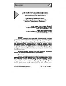
in which a project is planned hierarchically, is more appropriate. For this purpose, one can use a project work breakdown structure. A work breakdown structure (WBS) is a chart in which the work is iteratively split into smaller pieces. A lower level in the WBS corresponds to more detailed information. In this way sub-tasks can be divided and material and capacity requirements can be re…ned. In Figure 1.1, we show an example WBS.In general, a WBS

Project Work package

Work package

Activity Activity Activity Activity Activity

Work package Activity Activity Activity

Figure 1.1: Work breakdown structure. may have a variety of forms and there is no restriction to the number of levels. However, in order to limit administration and coordination e¤orts, the number of levels for planning and scheduling purposes should be as small as possible. In this thesis, we concentrate on three WBS levels, corresponding to projects, work packages and activities. In order to deal with uncertainty, Platje [56, 57] proposes that planning at separate levels should be tackled in a di¤erent fashion. Starting with an empty WBS, more detail is added in the course of the project. In the order acceptance stage, the work packages are de…ned. For each work package rough estimates of capacity requirements are made and critical items are identi…ed. These data are used as input for a rough-cut capacity plan. During the engineering and process planning stage, work packages are subdivided into various activities. Only after this information becomes available, an activity schedule can be generated. Platje makes a clear distinction between rough-cut capacity planning and activity scheduling, because entities and constraints are di¤erent. This view is clearly underlying our work as well. At the rough-cut capacity planning level, we do not actually consider workers and machines,

1.6 Project Management Theory - A Quantitative Approach

13

but computations are based on aggregate data. In Chapter 5, we will discuss the di¤erences between the two levels in more detail.

1.6

Project Management Theory - A Quantitative Approach

The quantitative trend in project management and scheduling theory focuses on quantitative analysis and decision making based on mathematical models and optimization techniques. The most popular quantitative tools for project management are network techniques such as the critical path method. In the last decades, also resource-constrained project scheduling problems receive increasing attention in literature. Other problems covered in the literature include time-cost scheduling and network models with discounted cash ‡ows. Techniques to solve the problems are based on operations research, such as linear programming and scheduling. In this thesis, we try to identify important elements that are lacking in these problems, and propose solution methods that are partly based on existing methods.

1.6.1

Project Network Techniques

Several techniques have been developed to assist management in planning and controlling projects. Most of these techniques are based on a graphical representation of the project network. Two alternative ways of representing a network by a graph occur in literature: the activity-on-arc model (AOA) and the activity-on-node (AON) model. We will demonstrate both models by a simple example, the data of which are represented in Table 1.1. We say that Ai is a predecessor of activity Aj , if activity Aj can only start after Ai is completed. Alternatively, one may say that activity Aj is a successor of Ai . The set of predecessors of activity Aj is depicted by Pj . Figure 1.2 demonstrates an AON representation of the project network.The nodes represent the activities and the arcs represent the precedence relations. The numbers above or under the nodes are the activity durations. Let E be the set of all arcs, such that hAi ; Aj i 2 E means that Ai is a predecessor of Aj . A dummy start node and dummy end node, with zero duration, can be added if preferred. Node

14

Introduction Activity (Aj ) A1 A2 A3 A4 A5 A6

Duration (pj ) 2 3 1 4 2 1

Predecessors (Pj ) ¡ ¡ ¡ A1 ; A2 A2 ; A3 A4

Table 1.1: Example project data.

A0

A1

A6

A2

A4

A3

A5

A7

Figure 1.2: Sample AON network. A0 is a dummy start node which has a directed arc to all nodes corresponding to activities that have no predecessors. Likewise, arcs are added beginning in all nodes referring to activities that have no successor and ending in the dummy end node A7 . In general, when we have N activities, the dummy end node is AN+1 . An AOA representation of the example project is given in Figure 1.3.Here, the arcs represent the activities, while the nodes represent events (the result of starting/completing at least one activity). Dummy arcs, represented by dotted arrows, must be used if activities do not have the same successors. For instance A4 is a successor of activity A2 , but not of activity A3 : Therefore, dummy arc hE3 ; E5 i is added. Although there is no fundamental di¤erence between the AOA-model and the AON-model, we prefer AON networks, because they are easier constructed. Constructing an AOA project network is even referred to as ‘something of an art’ (Evans and Minieka [25]). This technique has lost much interest with

1.6 Project Management Theory - A Quantitative Approach

A1

E1

A2

E2

A4

E4

A6

15

E6

A5

E3

E5

A3

Figure 1.3: Sample AOA network. the increasing popularity of computer applications. Another advantage of the AON-model is that new constraints, like minimum time lags between activities, can conveniently be added. Convention prescribes several rules for the construction of AON project networks. We mention the most important ones, to which we adhere in this thesis: 1. The network structure should be consistent. It would, for instance, be illogical that activity A2 is a predecessor of A3 , A3 a predecessor of A4, and A4 a predecessor of A2 : In other words: the network should not contain any directed cycle. 2. Activities should be numbered in such a way that an activity has a number that is always greater than the number of a predecessor. This can easily be accomplished by an event numbering procedure: give an activity that has no predecessor the …rst number, then repeat giving the next number to an activity whose predecessors are numbered (such an activity exists if there are no cycles) until all activities are numbered. 3. The network should not contain redundant arcs. This means that if there exists, for instance, an arc hA2 ; A3 i and an arc hA3 ; A4 i, then there should be no arc hA2 ; A4 i : We will now describe some critical path scheduling techniques that are based on the network representation methods described above. They can be divided in time-based techniques and time-cost trade-o¤ methods (cf. Chase

16

Introduction

and Aquilano [14]). The two best-known time-based techniques, which have found a broad application in project management practice, are the program evaluation and review technique (PERT) and the critical path method (CPM). The basic goal of both PERT and CPM, both developed in the late 1950s, is to …nd the critical path(s) of a project. A critical path is made up of activities whose delay would always result in a delay of the total project. The original di¤erences between the two techniques were that PERT used the AOA model and three estimations of activity durations, namely an optimistic, pessimistic and most likely estimate, whilst CPM used the AON model and only the most likely estimate. These di¤erences re‡ect the origin of the methods: PERT was developed under sponsorship of the US Navy as to support management of the Polaris missile/submarine project, a very complex project, characterized by much uncertainty. CPM, on the other hand, was developed by DuPont to support the scheduling of fairly routine plant maintenance projects. Nowadays, often a mixture of both methods is used. Therefore, the di¤erence between CPM and PERT has become blurred. For convenience, we will only use the term CPM from now on. We now describe the CPM in case of a single time estimate. As we remarked, the CPM aims at …nding the critical path(s) of a project network. The length of a critical path gives the minimum duration of the project if all activities would start immediately after their predecessors. By de…nition, there ex® ® ists a path from Ai to Aj in the graph if there are arcs A[1] ; A[2] ; A[2] ; A[3] ; ® ® : : : ; A[¸¡2] ; A[¸¡1] ; A[¸¡1] ; A[¸] such that A[1] = Ai and A[¸] = Aj . We assign to each node Aj a weight of pj , namely the duration of Aj and to each arc a weight of zero. Let the weight of a path from Ai to Aj be the total weight of all nodes and arcs on that path, excluding the weight of Ai and Aj . A longest path between Ai an Aj is a path between these two nodes with a maximum weight. Given these de…nitions, a critical path in the project network is simply the longest path from A0 to AN+1 . Since there can be more than one longest path in a graph, there can also be more than one critical path in a project network. For longest path determination, a reversed version of Dijkstra’s Algorithm is mostly used (see, e.g., [25]). This procedure computes for each activity Aj

1.6 Project Management Theory - A Quantitative Approach

17

its earliest start time and its latest …nish time. The earliest start time ESTj is the earliest possible time Aj can start if all preceding activities are started directly after the completion of their predecessors. The latest …nish time LF Tj is the latest possible time to …nish Aj , without delaying the project. These values are computed as follows: Algorithm 1.1 Longest path algorithm. 1. 2. 3. 4. 5. 6.

Let EST0 à 0; FOR j = 1 TO N + 1 DO ESTj à maxi2Pj (ESTi + pi ) ; LF TN +1 à ESTN+1 ; FOR j = N DOWNTO 0 DO LF Tj à minfijAj 2Pi g (LF Ti ¡ pi ) :

The slack of each activity Aj is now de…ned as LF Tj ¡ ESTj ¡ pj . Essentially, the slack of an activity Aj is a quantitative measure that indicates how much an activity can be delayed, without delaying the completion of the whole project. A critical path is a path of activities between A0 and AN+1 that are critical, i.e. have a zero slack. In Table 1.2, it becomes clear that the critical path is made up of activities A2 ; A4 ; and A6 : The length of the critical path is ESTN+1 = 8.

1.6.2

The Resource-Constrained Project Scheduling Problem

In CPM and PERT, a critical path is based on activity durations and precedence relations. These techniques ignore capacity requirements of activities. Thus, they assume that in…nite capacity is available. Of course, this is a highly unrealistic assumption, since in practice activities must be performed by resources such as people and machines. Most of these resources have a limited capacity, at least in the short term. We will illustrate the e¤ect of resource constraints by adapting the example project of the previous section (see Table 1.1). Activity durations and precedence relations are the same, but

18

Introduction Activity (Aj ) A0 A1 A2 A3 A4 A5 A6 A7

ESTj 0 0 0 0 3 3 7 8

LF Tj 0 3 3 6 7 8 8 8

Slack 0 1 0 5 0 3 0 0

Table 1.2: Results of CPM. we assume that we have one resource with four resource units (e.g., workers with a certain skill) available to perform the project. For the execution of each activity, a number of units is required. Table 1.3 displays the resource requirements of each activity. If we ignore that the available capacity is limited Activity (Aj ) A1 A2 A3 A4 A5 A6

Duration (pj ) 2 3 1 4 2 1

Units required (qj1 ) 3 1 2 2 3 3

Table 1.3: Activity duration and capacity requirements. to four resource units and schedule each activity at its earliest start time, we obtain the schedule presented in Figure 1.4.It is clear that this schedule cannot be realized with the current availability level. Moreover, there is no schedule that completes this project in eight days with a capacity of four resource units. This can only be done if at least one extra resource unit will be added. When capacity constraints are given, the critical path method gives a lower bound to the project duration, but there is a high probability that this duration cannot be actualized. The resource-constrained project scheduling problem (RCPSP)

1.6 Project Management Theory - A Quantitative Approach

19

A3 4

A5 A1

2

A2 0

A6

A4

2

4

6

8

10

Figure 1.4: Capacity constraints ignored.

4 A1

2

A3

A2 0

2

A6

A4 4

6

8

A5 10

Figure 1.5: Resource-constrained project schedule. aims to …nd a project schedule with minimum duration, taking into account precedence relations and capacity constraints. Figure 1.5 shows an optimal schedule for the example instance.The general RCPSP is not bounded to one resource but it considers multiple resources. Unlike the critical path problem, the RCPSP is, in general, very hard to solve. In Chapter 3, we discuss the RCPSP in more detail and present some procedures to solve it. Generally speaking, one could say that the quantitative approach in project management literature focuses on describing and solving isolated, often theoretical problems. Many situations that occur in (semi-)project-driven organizations are not covered (see Chapter 4). Another striking observation is

20

Introduction

that, to the best of our knowledge, no distinction is made between di¤erent levels of capacity planning. Literature presents no useful techniques to deal with the combination of limited capacity and structural uncertainty in an effective manner and multi-project rough-cut capacity planning is not explicitly dealt with. In this thesis, we provide a new coherent framework to do so.

1.7

Project Management Software

We discuss four categories of production planning systems that are used by many production organizations: MRP-based systems, …nite capacity scheduling systems, and project management information systems. The …rst category represents enterprise resource planning (ERP) packages based on the MRP philosophy. Useful as ERP-systems may be for many information processing tasks in an organization, they provide insu¢cient support in resource constrained multi-project planning. One of the major problems with MRP is that it uses constant lead times as input for the planning and that it assumes in…nite capacity. However, with limited capacity, lead times are a result of resource loading. Thus, lead times should be output of the planning, not input. Even MRP II does not provide a good solution to this problem (see, e.g., Hopp and Spearman [35]). Moreover, MRP was never developed for the environments we are discussing in this thesis. In general, project-driven companies are typically engineer-to-order and make-to-order companies. The MRP philosophy, on the other hand, was intended for make-to-stock environments. Finite capacity scheduling systems make up the second category. These systems are mainly developed for shop ‡oor scheduling. Most of these systems employ priority-rule based scheduling rules, while some are based on sophisticated scheduling algorithms (see, e.g., Schutten [63]). They do, however, not support resource-constrained project scheduling, in which multiple resource units are required for an activity (see Section 1.6.2). Moreover, they do not support top-down capacity planning. The third category consists of project management information systems (PMISs), of which many commercial variants are available. Although intended

1.8 Project Management in Practice

21

for practical project management, they do not o¤er the required insight nor the ability to make high quality decisions. Many PMISs were only developed for single projects, or they can deal with multiple projects via awkward consolidation procedures only. Existing PMISs can only take into account capacity requirements at the activity level. This means that the top-down planning, described in Section 1.5.2, is not possible. Another shortcoming of generally available PMISs is that their resource constrained scheduling possibilities are insu¢cient. Some of the packages have …nite resource scheduling or resource leveling options, but they are based on simple single-pass priority-rule based heuristics and therefore often result in inferior schedules. Moreover, these algorithms are very basic and do not reckon with practical extensions such as multiple execution modes for activities, changing capacity pro…les and spatial resources (see Chapter 4). Since capacity is only accounted for at the activity level, no computational support is available for planning at a higher capacity level for due date quotation or subcontracting/hiring decisions. It would be unfair to blame only software developers for these shortcomings in available information systems. Many of the problems mentioned above are just not covered in project management and scheduling theory, or they are dealt with only fragmentized. This thesis is an attempt to specify the most important functional requirements of an automated planning system for (semi-)project driven organizations. For this purpose, we introduce extensions to existing scheduling theory and describe a prototype decision support system in which these functional requirements are implemented.

1.8

Project Management in Practice

Today, there exist only few areas in which project management has no application. Whether it is in marketing or production, in pro…t or non-pro…t organizations, at work or at home, projects are found everywhere. In many of these cases, no complicated management or scheduling techniques are required, since part of the project objectives are rather ‡exible or trade-o¤s are

22

Introduction

easy to make. Sometimes, for instance, the time required to complete the project is much less important than the outcome. In such situations, it is not pro…table to use sophisticated techniques for a project’s completion time estimation or putting much e¤ort in the construction of a feasible project schedule. However, one may think of project-based environments where management is much more complicated and considerable amounts of money are involved. Quoting tight, yet reliable due dates at a lowest possible cost and realizing them may be of vital importance in many cases. In this section, we brie‡y describe some real-life project management environments, in order to detect the major problems that management faces in these situations and to stress again the shortcomings of project management software. We will start with some results found by a survey reported in literature, in order to determine some general characteristics of projects in di¤erent industries. Next, we will brie‡y describe the cases of the Netherlands Navy Dockyard where projects form a crucial part of the primary process.

1.8.1

Surveys of Projects in Diverse Industries

Icmeli-Tukel and Rom [36] performed a study on the characteristics of projects in various industries. From their survey, they conclude, among other things, that 45% of the projects have less than 100 activities, and that labor hours are regarded as the resources most critical to project success. From this fact, they conclude that, in general, e¢cient exact algorithms should be preferred to heuristic methods. We do not share this conclusion, since the majority of projects (55%) consists of 100 activities or more, and the same survey also reveals that only 7% of the projects are implemented as single projects, whereas the majority of projects (60%) was implemented in parallel with at least …ve other projects. In 95% of the cases, man hours were shared among parallel projects. Qualitatively good schedules can only be achieved if an algorithm simultaneously considers all projects sharing common resources. Since the majority of cases cover at least 200 activities, heuristic solutions seem more appropriate. This is the approach we will take in this thesis. Another result was that for most project networks (75%) the average number of immediate predecessors is between 2 and 5 and that for 60% of the

1.8 Project Management in Practice

23

projects this density is equal for di¤erent stadia of the project, thus resulting in a centered network. The life span of the projects range from less than 2 months to more than 5 years and 71% of the projects are completed within two years. The approximate value of projects ranges from less than 10,000 US$ to more than 10 million US$, with the most common value (25%) in the US$1-US$5 million range. Exceeding projects’ due dates practically always results in a negative e¤ect of some kind. The survey indicates that loss of credibility (or goodwill) was the most experienced penalty (67%), followed by monetary penalties (46%) and loss of a customer (26%). Still, 54% of the respondents state that project deadlines are often not met. This may partly be caused by the fact that deadlines are often imposed exogenously (49%) and delays are sometimes due to contractors (51% indicate that more than 10% of the delays is due to contractors). It is remarkable however, that software packages are used for estimating project completion times in only 20% of the cases. Unfortunately, the survey does not specify how often …nite capacity scheduling and resource leveling functionalities were used in these cases. The criteria that were used to measure projects’ success were: quality (77%), client satisfaction (74%), time (73%), and cost (68%). Factors that are regarded as most important to the project’s success are: su¢cient resources (78%), top management support (73%), and the project manager’s performance (60%). Although some questions still remain unanswered, the results of this survey justify a sophisticated approach for better utilization of resources and improved due date performance.

1.8.2

Project-Based Management at the Royal Netherlands Navy Dockyard

The research in this thesis was mainly inspired by the Royal Netherlands Navy (RNN) Dockyard, located in Den Helder, The Netherlands. In this section, we will give an indication of the major problems this company is facing. In Chapter 7, we describe the RNN Dockyard in more detail and report some test results on a prototype decision support system we developed in cooperation

24

Introduction

with this dockyard. The one customer of the RNN Dockyard is the Royal Netherlands Navy (RNN). The dockyard is, among other things, responsible for the maintenance, overhaul, and modi…cation of the ‡eet as well as shore facilities of the Netherlands Navy. As we discussed in Section 1.1, project management is suitable in low-volume production environments with diverse routings and multiple resources. These characteristics apply to a signi…cant part of the order portfolio of the dockyard. Therefore, the RNN Dockyard may be classi…ed as a semi-project-driven organization. The main characteristics of the RNN Dockyard are that projects are always initiated by the customer and that multiple projects are always overlapping and thus compete for shared resources. The most bounding resources are labor, special heavy equipment, and spatial resources, such as a dry dock. The dockyard strives for shorter lead times and a better due date performance, but has a hard time in realizing this because of complexity and uncertainty in the planning process. Existing software packages do not o¤er the required support in taking the most important decisions, such as: what due date should be quoted to the customer? When and how much should capacity be expanded by working overtime, hiring or subcontracting. Which activities are critical? What are the consequences of a rush order, or a major disturbance in the planning? How do we prioritize projects and subsequent activities correctly, without running into trouble later on? A clear hierarchical framework for capacity planning is lacking and existing information systems do not o¤er the required support in the important management decisions described above. The RNN Dockyard is not the only company that is confronted with these problems. We have come across a variety of companies that face similar problems, in particular engineer-to-order and make-to-order companies where products or services require multiple resources and activity networks are complex. At one other company, the Peters Shipyard, located in Kampen, The Netherlands, our prototype decision support system was also tested (cf. Wijdeveld [73]).

1.9 A Decision Support System for Multi-Project Management

1.9

25

A Decision Support System for ResourceConstrained Multi-Project Management

From the preceding sections, we may conclude that project management theory does not provide su¢cient support for management of (semi-)project-driven organizations. Although some ideas have been suggested about a hierarchical approach to capacity planning, a profound description of the problems and accompanying information requirements at each level are not given. Project scheduling theory focuses on theoretical problems that ignore some important elementary factors that occur in many real-life situations. In our research, the goal was to …ll the gap between theory and practice by constructing a hierarchical framework for resource-constrained multi-project management, modeling the problems that occur at di¤erent levels and developing fast algorithms that give good quality solutions to these problems. Above all, the research should address the important decisions that must be made in a resource-constrained multi-project environment, the information that is required for these decisions, and propose how this information can be presented to the decision maker in a simple and convenient way. In brief, the main objective of the research presented in this thesis is: The design of a decision support system (DSS) to assist management of resource-constrained (semi-)project-driven organizations in making planning and scheduling decisions. This system must be based on a top-down approach in order to reckon with the lack of detailed information in early project stages. Furthermore, Operations Research techniques will be employed that take into account important constraints that occur in practical situations. This DSS should support the management of (semi-)project-driven organizations in several tasks, such as order acceptance, priority setting, capacity management, resource scheduling, and performance evaluation with a primary focus on due date performance. The algorithms and functionalities proposed in this thesis must be implemented in a fully interactive prototype in order to validate the design to practical situations.

26

1.10

Introduction

Overview of the Thesis

The remainder of this thesis is organized as follows. In Chapter 2, we discuss the organizational context in which the DSS should function and we present a framework for hierarchical planning in (semi-)project-driven organizations. Chapter 3 describes the standard resource-constrained project scheduling problem (RCPSP) and gives an overview of existing solution procedures to solve this problem. The standard RCPSP is, however, a theoretical problem that ignores several important constraints that occur in (semi-)project-driven organizations. In Chapter 4, we present the most important extensions we came across in practice. Moreover, we present a heuristic to solve the extended RCPSP, based on the Adaptive Search Method of Kolisch and Drexl [45] and present computational results. This heuristic, that can be used for scheduling activities, requires relatively detailed input data, which are often not available in the order acceptance stage of a project. Chapter 5 introduces the MultiProject Rough-Cut Capacity Planning Problem (RCCP) that corresponds to the next higher planning level. We present heuristics for both the resource driven RCCP and the time driven RCCP and conclude the chapter with computational results. In Chapter 6, we give an outline of the major tasks of the DSS and show an architecture representing the major functions and components of the prototype DSS. Chapter 7 reports on the development and implementation of the prototype DSS at the Royal Netherlands Navy Dockyard as well as the organization wide reengineering project that gave rise to the DSS. Finally, we end this thesis with some conclusions and recommendations for further research in Chapter 8.

27

Chapter 2

A Framework for Hierarchical Planning in (Semi-)Project-Driven Organizations 2.1

Introduction

Before designing the decision support system for resource-constrained multiproject management, we will …rst consider the organizational context for which it is intended. For this purpose, we start by describing coordination mechanisms that make up an organization and show how some of these mechanisms can be e¤ective in (semi-)project-driven organizations. Next, we propose a framework for hierarchical planning in (semi-)project-driven organizations and show the resulting decisions and actions in each project stage. Section 2.6 concludes the chapter. This chapter is inspired by and partly based on De Waard [20]. For more details on the organizational aspects of large semi-project-driven organizations, we refer to his work.

2.2

Coordination Mechanisms for Complex Organizations

If a group of people wants to cooperate in performing a certain task, this task should be broken down in various sub-tasks and these sub-tasks should

28

A Framework for Hierarchical Planning

be linked. The structure of an organization is thus determined by two key concepts: division of labor and coordination. Adam Smith [65] showed how productivity can be improved dramatically by dividing a task into many subtasks and thus realizing job specialization. This e¤ect is limited however, since too much job specialization may have a negative e¤ect on a worker’s motivation. Anyway, increasing division of labor means that more coordination is required. Mintzberg [50] distinguishes …ve mechanisms by which coordination between sub-tasks can be achieved: ² Mutual adjustment. The simplest way of coordination is informal communication by executors of the sub-task. Mutual adjustment is naturally used in very simple organizations, such as two hairdressers who run a barber’s shop jointly. Paradoxically, it is also used in the most complex organizations, since it is often supposed to be the only mechanism that works in very di¢cult situations. ² Standardization of work processes. An alternative way to achieve coordination is by specifying the contents of the work that has to be done. Work standards can be very narrow, such as a recipe in a cookbook, or leave some autonomy by specifying boundaries only. ² Standardization of outputs. Often it is not necessary to tell someone how he should perform a certain task. Merely specifying the results of the work can be enough. This way of coordination ‘brings the point of decisions to the point of action’ by setting, for instance, performance targets or dimension tolerances. Other names for this mechanism are targeting or goal setting. ² Standardization of skills. Another form of coordination is standardization of skills and knowledge. This can be achieved by specifying the kind of training or education that is required. ² Direct supervision. If the number of people working together increases, mutual adjustment would take too much time. The coordination mechanisms of standardization were by de…nition intended for standard

2.2 Coordination Mechanisms for Complex Organizations

29

situations. They are not adequate in case exceptions occur, e.g., when a new task has to be performed or a speci…ed output cannot be met. In case of such unanticipated events, a decision should be made that considers all sub-tasks that are involved. Thus, one individual takes responsibility for the work of others by issuing instructions and monitoring their work. In this way, coordination is achieved by creating a hierarchy with managerial roles. Galbraith [26] states that the structure of an organization is e¤ective only if it is tailored to the uncertainty of its tasks. He de…nes uncertainty as ‘the di¤erence between the amount of information required to perform the task and the amount of information already possessed by the organization’. The volume of information depends on the diversity of the outputs, the number of di¤erent input resources required, and the performance level aimed for. The greater the uncertainty of a task, the more information has to be processed between participants in order to achieve a given performance level. It is not only the amount of uncertainty, but also the timing of uncertainty that in‡uences coordination. The later information becomes available, the more complex coordination will be. If much of the task is known prior to performing it, a reliable schedule can be made, although this may require quite some information processing. However, if the task is not well understood, then more information becomes available during the execution of the task, leading to changes in resource allocations, schedules, and priorities. Mintzberg’s coordination mechanisms only work e¤ectively to a certain extent. If organizations are too large for coordination by mutual adjustment, a hierarchy is required to deal with uncertainty. Information must be collected and decisions must be made to cope with unanticipated events that a¤ect various sub-tasks. A problem with hierarchical structures, however, is that each channel has a limited capacity for information handling. If there is too much task uncertainty, a great number of exceptions may cause an overload in the hierarchy, causing substantial delays in communication and decision making. More decision authority may be delegated downward the hierarchy by goal setting (standardization of outputs) and profesionalization (standardization of skills), but since sub-tasks are usually linked to other sub-tasks, this may

30

A Framework for Hierarchical Planning

lead to decisions that are only optimal from a local point of view. If the amount of information required for coordination of sub-tasks exceeds the capacity of an organization’s structure, then the organization must take actions to either reduce the need for information or increase the information processing capacity of its hierarchy. Galbraith proposes four design strategies to prevent hierarchies from overloading. We describe how these strategies can be employed in (semi-)project-driven organizations: ² Creation of slack. The number of exceptions that occur as a result of not meeting output targets can be reduced by simply lowering these targets. This may result in longer lead times, increasing work in process levels, under-utilized labor and machine capacity, or lowering quality standards. In each case a cost is paid by either the organization or the customer who gets less value for money or must wait longer. However, the lower the performance targets, the lower the probability that they will not be met. Thus, the creation of slack reduces the need for vertical information processing in the hierarchy. It is not necessarily wrong to create slack, because it may reduces the complexity of coordination signi…cantly. However, the cost of slack resources may reach unacceptable proportions. Moreover, organizations often do not realize that this slack occurs. We think that in (semi-)project-driven organizations some slack may be built into a schedule to reduce the number of exceptions to the original schedule. However, slack must be used in a controlled way. This means that it may be added in one project stage only, that it must be quanti…ed and made visible to management and that it must be kept small by employing smart planning methods. ² Creation of self-contained activities. In a functional structure, work orders are usually designed in such a way that they can be performed by one expertise group. For this reason, work orders are relatively small and much coordination is required among them. With a minimal use of slack, this will result in an overload of the hierarchy. A way to relieve the hierarchy is by de…ning larger tasks that can be executed by a multi-disciplinary team, namely self-contained activities. Work coordination within such an activity must be based on mutual adjustment

2.2 Coordination Mechanisms for Complex Organizations

31

between team members, thus reducing the need for coordination by direct supervision. The activities have to be designed such that they form a coherent work cluster, e.g., based on systems or rooms. This is necessary to minimize interference between activities. On the other hand, activities may not be too large, otherwise coordination based on mutual adjustment will become impossible and monitoring progress will be too hard for management. A positive e¤ect of self-contained activities will be the reduction of division of labor. Depending on the way teams are put together, people will perform more di¤erent tasks and have more control over their work, thus causing job enlargement and job enrichment. This may result in motivated and more ‡exible (multi-skilled) workers. There are many ways in which multi-disciplinary teams may be formed. Decision variables, including size, homogeneity, and life-span of a team, have a major impact on resource utilization, ‡exibility, and worker motivation. ² Creation of lateral relations. While the two previous described strategies aim at reducing the need for information processing, there are also two strategies that can increase the information handling capacity of a hierarchy. One of these strategies is the utilization of lateral linkages or liaison devices (cf. Mintzberg [50]). This means that managers from di¤erent organizational units solve common problems at their own level, instead of referring them upward in the hierarchy. Two liaison devices that can be of use in (semi-)project-driven organizations are the matrix structure and the standing committee. The matrix structure, which we brie‡y discussed in Section 1.5.1, avoids choosing one prevailing basis for grouping. Instead, it chooses two bases for structuring the organization, often projects and functional departments. A standing committee is a group of people that meets regularly to discuss questions of common interest and has a permanent character. It often exists at middle echelons of organizations. In project-driven organizations, a standing committee can be an e¤ective instrument for coordination among parallel projects. Platje and Seidel [58] propose such a standing committee and call it the portfolio management team. This team consists of project managers and

32

A Framework for Hierarchical Planning managers of functional divisions. In the next section, we will elaborate on the matrix structure and the portfolio management team. ² Investment in vertical information systems. Another strategy that can increase an organization’s capacity to process information and make decisions is the use of (vertical) information systems. Contemporary information and communication technology o¤ers huge potential to facilitate exception communication, data collection, decision making, and issuing new targets or schedules. Not only can information systems speed up the decision and communication processes, but in many cases also the quality of decisions can be improved by using decision support systems employing fast and powerful algorithms. The goal of this thesis is to design a decision support system that assists the portfolio management team in taking coordination decisions, in particular planning and scheduling. Other systems that can increase information processing capacity and support coordination are a shop ‡oor control system for the management of functional divisions and a database with estimations of capacity requirements and durations for standard activities, in order to accelerate process planning. In Chapter 6, we will describe these systems and their relation to the decision support system in more detail.

In the remainder of this thesis, we assume that the creation of self-contained activities, the matrix structure and the portfolio management team are e¤ective coordination strategies for (semi-)project-driven organizations with much uncertainty. For this reason, we concentrate on organizations whose structures are based upon these strategies.

2.3

The Matrix Structure and the Portfolio Management Team

In many (semi-)project-driven organizations, the organizational structure is a combination of a purely function-based and a pure project organization. Such a matrix structures is an attempt to combine the advantages of both. However, with this structure, the principle of unity of command is sacri…ced. This

2.3 The Matrix Structure and the Portfolio Management Team

33

means that an individual may have di¤erent superiors: a functional manager and one or more project managers. In order to avoid too much ambiguity, it can be useful to distinguish three areas of direct supervision, namely, hierarchical, functional and operational (Van Aken [71]). Hierarchical supervision involves all aspects of salary, training, and the career path of the subordinate. Functional supervision is concerned with how tasks should be performed, while operational supervision relates to which tasks should be performed and when. In cases of potential ambiguity, it can be useful to formalize the roles of various members of the organizations by responsibility charting. Using this technique, responsibility for decisions can be assigned to positions in the organization. Matrix organizations either have a permanent or a shifting structure. A shifting matrix structure, is an organization were interdependencies, units, and people shift on a regular basis. Such a structure is most adequate where output frequently changes. Although the coordination in a shifting matrix structure is more complex, it o¤ers more ‡exibility and a higher utilization of resources. In a shifting matrix structure, projects implemented in parallel are likely to interfere with each other, since they compete for shared resource. In case of semi-project-driven organizations, there are also ‘common’ orders, i.e., orders that are not carried out through projects. Since several projects and common orders are competing for the same resources, it is important that the right priorities are assigned to them. Also, reliable due dates must be quoted for new work. Furthermore, when serious disruptions in a schedule occur, right decisions must be made concerning the delay of certain activities or the use of extra resources. These decisions a¤ect all divisions of the organization. Thus, it is impossible for one person to oversee all the consequences. A portfolio management team can be an e¤ective vehicle to facilitate coordination in such a complex organization. This team consists of project managers, product managers, and managers of functional divisions (see Figure 2.1), representing implemented projects, common orders and organizational resources. Basically, the function of the portfolio management team is to match the supply and demand of capacity. The portfolio management team regulates and formalizes the communication between managers that must take place in order to coordinate the work and …nd agreement on topics of con‡icting interest. The team

34

A Framework for Hierarchical Planning

Portfolio Manager

Resource Manager 1

Resource Manager 2

Resource Manager 3

Project Manager 1 Project Manager 2 Project Manager 3 Project Manager 4 Project Manager 5 Product Manager 1 Product Manager 2

Figure 2.1: Portfolio management team. meets frequently, e.g., fortnightly, and makes decisions on the basis of mutual adjustment. A portfolio manager must be present to facilitate the discussion and to solve deadlocks. Decisions that are made at the portfolio management level are often complex: it is di¢cult to design good feasible schedules, taking into account all important constraints. It is also di¢cult to estimate consequences of changes in the schedule of one project to, e.g., the completion times of other projects. In order to improve the quality and speed of decision making, we propose a decision support system for the portfolio management team. This system must employ smart algorithms that deliver good quality solutions in little time. Since not all constraints and objectives are quanti…able, the decision support system must be able to represent di¤erent scenarios in order to support what-if analyses. Schedules and consequences of decisions must be shown by convenient graphical outputs, in which several tools support the analysis of (potential) problems. In the next section, we present a framework for hierarchical planning in (semi-)project-driven organizations. This framework makes clear what kind

2.4 A Framework for Hierarchical Planning

35

of decisions the portfolio management team should take. Therefore, this hierarchical framework is a basis for designing the decision support system.

2.4

A Framework for Hierarchical Planning

In order to break down planning into more manageable parts, hierarchical planning frameworks have been proposed for several environments. Most of these hierarchical production planning (HPP) models distinguish at least three decision levels, corresponding to strategic, tactical, and operational decisions. At each level, the constraints are set for subsequent levels. This means that going down the hierarchy reduces the decision space and results in more structured problems. In most multi-project environments, it makes no sense to plan all work at one level, since collecting all the required information would, if possible at all, take too much time. Furthermore, much information would be inaccurate, since uncertainty plays an important role. Working with aggregate data for long-term, high-level decisions is more appropriate. After all, time and capacity estimates of a set of activities tend to be more accurate than estimates of each individual activity. Generally, more information becomes available when time goes by, thus the longer the period on which decisions must be taken, the more uncertainty in the information will play a role. Hopp and Spearman [35] state that ‘problems at di¤erent levels of the organization require di¤erent levels of detail, modelling assumptions, and planning frequency’ and that ‘planning and analysis tools must be consistent across levels.’ It is therefore remarkable that project scheduling theory hardly concentrates on problems at multiple levels. We propose four levels for planning: 1. Strategic resource planning; 2. Rough-cut capacity planning; 3. Resource-constrained project scheduling; 4. Detailed scheduling.

36

A Framework for Hierarchical Planning

Strategic resource planning

Strategic

Tactical

Rough-cut process planning

Rough-cut capacity planning

Tactical/ operational

Engineering & process planning

Resource-constrained project scheduling

Operational

Detailed scheduling

Figure 2.2: Hierarchical planning framework. These levels make up a hierarchical planning framework for (semi-)projectdriven organizations displayed in Figure 2.2. Each level uses its own input data, planning horizon (length of time span for which decisions are made) and review interval. The objective of strategic resource planning is to determine the organization’s global resource capacity levels. At this level, strategic decisions are made with regard to space, sta¢ng levels, layouts, number of machines and other critical resources. A strategic resource plan should be preceded by setting corporate goals, and performing an external and internal analysis of the organization (see, e.g., Hill and Jones [34]). Other input data may be market research reports, agreements with major customers, and management vision with regard to strategic issues, such as the maximum amount of subcontracting and the acceptable level of underutilization, in line with the corporate mission. The planning horizon of such a plan may vary from one to several years and the review interval should depend on the dynamics of the organization’s environment. At the rough-cut capacity planning (RCCP) level decisions are made about due dates and milestones of projects, overtime work levels, subcontracting, and so on. The RCCP should be used during the bidding and order accep-

2.4 A Framework for Hierarchical Planning

37

tance phase of a new project. Two approaches to the RCCP problem can be distinguished: resource driven and time driven planning (see Möhring [51]). With resource driven planning, the availability of each resource is constrained, and the aim is to meet due dates as much as possible. On the other hand, with time driven planning, time limits on the projects are given, and the aim is to minimize the use of non-regular capacity, such as overtime work. In Chapter 5, we discuss both RCCP problems more extensively. In practice, a combination of the two methods may be used. In order to generate input for the RCCP, some kind of rough-cut process planning has to take place (see Figure 2.2). Based on customer speci…cations, this rough-cut process planning should result in a network of work packages with rough estimates of resource requirements (e.g., in man-hours) and minimum durations. The minimum durations are a result of technical constraints, such as available working space and expected precedence relations between activities at a lower level. This network, together with project networks already available and estimations of future resource availabilities, is input for the RCCP. In the case of time driven planning, deadlines should be part of the input. The planning horizon of the RCCP procedure should be half a year or more, depending on expected project durations. The next level corresponds to the resource-constrained project scheduling (RCPS). After a project is accepted, more detailed information about resource and material requirements becomes available from engineering and process planning. On the basis of this information, a more detailed activity network can be drawn. The work packages of the RCCP level are broken down into smaller activities with constant duration and resource rates (e.g., number of men required from a certain resource group). In addition, precedence relations between activities are speci…ed. An activity must be performed by one multi-disciplinary team. Together with detailed resource availability pro…les determined at the RCCP-level, these data are input for the RCPS. The planning horizon of the RCPS procedure may vary from several weeks to several months. The RCPS should be updated whenever new facts are known, for example when process planning results in a new cluster of activity data or when a major disturbance on the work ‡oor occurs. A more elaborate description

38

A Framework for Hierarchical Planning

of the RCPS problem and its extensions, is given in Chapter 3 and Chapter 4. The RCPS determines when activities are performed by certain resource groups, but the schedule does not necessarily indicate which persons or machines of that group are assigned to each activity. For this purpose, detailed scheduling (or manpower scheduling or shop ‡oor scheduling) should be used. The resulting schedule speci…es which persons (by name) or which machines will work on a speci…c activity at a certain time. Thus, a detailed schedule assigns a multi-disciplinary team to each activity. The planning horizon of the detailed scheduling procedure may vary from one week to several weeks. It should be updated fortnightly, every week, or more often, depending on changes in the RCPS and on the situation on the shop ‡oor. The preceding description of the decision levels indicates which information is passed to subsequent levels, such as resource capacity levels and due dates. This information, which often imposes constraints on lower levels, ensures downward compatibility of the framework. In order to ensure upward compatibility, feedback loops are integrated in the framework (see Figure 2.2). Each time a major disturbance in production occurs, the detailed schedule should be updated. If this results in a violation of project deadlines or other milestones, a revised RCPS is needed. If resource requirements for some activities are drastically underestimated or major delays occur, it may be necessary to update even the RCCP in order to improve the order acceptance and quotation process. The importance of these feedback loops increases if the degree of repetitiveness of activities is low: if an organization has never performed a certain task before, it is often di¢cult to estimate its duration and resource requirements accurately.

2.5

Coordination at Each Project Stage

In this section, we show the impact of the hierarchical framework on the actions to be taken at each project stage. These actions should facilitate an e¢cient project implementation and a high due date performance. In order to prevent the organizational hierarchy from a coordination overload, we integrate this framework with a shifting matrix structure, self-contained activities, and a

2.5 Coordination at Each Project Stage

39

portfolio management team. In Chapter 6, we show how the decision support system may assist the portfolio management team in some of the project stages. The description of the project life cycle stages, based on Section 1.4, focuses on relatively large projects. In case of small projects, some phases may be skipped or shortened.

2.5.1

Order Acceptance

The order acceptance phase corresponds to the RCCP level in the hierarchical framework. In this phase, the customer informs a sales representative about the desired end-results in the form of functional speci…cations. Based on these descriptions, the organization must quote a price estimation and a delivery date. In order to make reliable, yet competitive estimations, a rough-cut capacity plan must be developed. This means that a network of work packages with rough estimates of required capacity and minimum durations must be designed (rough-cut process planning). This network must cover all the work of the order, including preliminary tasks such as engineering and process planning. In many cases, one or more projects with at least some similarities have been performed in the past, hence historical data of these projects may be used to get more accurate estimations. If critical items (i.e., items with a long delivery lead time) are required, start-milestones must be de…ned, indicating that some work packages cannot start before these items are available. The resulting work package network must be planned such that the resulting lead time is minimized, taking into account available resources, work already accepted, milestones, precedence constraints and possible reservations for expected work. Based on this plan, a due date can be quoted to the customer. If the customer does not agree with this date, a plan must be made in which a minimum amount of extra resources is employed such that a due date speci…ed by the customer is met. If the customer and the sales representative come to an agreement, the order is accepted and a contract is signed. In certain cases, it may be necessary to discuss several options in the portfolio management meeting, e.g., in order to reset priorities among orders.

40

2.5.2

A Framework for Hierarchical Planning

Engineering and Process Planning

Process planning implies the translation of functional requirements of the customer into a network of activities. Functional requirements only state the desired end-result (‘what’), while the process planner speci…es which resources and methods may be employed to realize these end-results (‘how’). Process planning should yield the required input for the scheduling phase. These are for each activity: a description of work to be done, its duration, resource requirements, precedence relations, and materials required. Often an activity can be executed in several di¤erent modes, requiring di¤erent duration/resource combinations. If this is the case, the modes should be speci…ed. It is important to note that activities are not given a start or completion time yet, nor is a mode assigned to an activity. No schedule is generated in this phase, only input for the scheduling phase is generated. In complex environments, people sometimes have the tendency to specify activity start and completion times and accompanying modes during the process planning phase. However, this may result in schedules with a poor performance, or even infeasibilities with regard to resource and precedence constraints. In process planning, only ‘real’ constraints should be speci…ed to give the scheduler as much freedom as possible. Even in engineer-to-order environments, a signi…cant amount of work that must be done is often identical or similar to previously performed activities. For this kind of work, process planning may be accelerated by using a database of standard activities. Filling this database and keeping it up-to-date often is a huge job, but it may cut down process planning time signi…cantly and thereby reducing total lead times as well! Moreover, it is a great opportunity to critically look to the way work must be carried out and possibly redesign work methods, thus increasing e¢ciency and speed. Work that was not performed before usually requires engineering or designing activities. A sound rough-cut capacity plan includes time for these activities as well: in many companies, the engineering department is a critical resource. If necessary, special documentation, such as drawings, quality speci…cations and safety regulations must be provided during this phase. Note that in the engineering and process planning stage, a focus on time

2.5 Coordination at Each Project Stage

41

is important in two ways. In the …rst place, engineering and process planning takes time and consumes resources. Therefore, these tasks should be included in the rough-cut capacity plan and monitored, just as production tasks. Secondly, process plans induce constraints for the scheduling phase. Activity durations and precedence constraints determine the minimum project duration. In addition, some resource selections may result in the overloading of certain resources, thus increasing project duration. Therefore, the organization must pay severe attention to e¢cient work methods and materials and equipment selected.

2.5.3

Material and Resource Scheduling

Scheduling in this phase corresponds to the RCPS in the hierarchical framework. Input for the scheduling phase are the activity network, including capacity and material requirements, designed at the process planning phase, activity networks of all other implemented projects, and resource availability pro…les. In the order acceptance phase, planning was based on rough estimates. During process planning, more accurate and speci…c data has become available. Moreover, as a result of the planning horizon, resource capacity levels can usually be adapted at the RCCP level, whilst they are practically given at the RCPS level. Most activities require several skills from di¤erent functional units, i.e., they require a multi-functional team. Therefore, we have a resource-constrained multi-resource scheduling problem. The aim of the scheduling phase is to determine a start and completion time for each activity and to select an execution mode in which it will be performed. There may exist di¤erences between the schedule and the rough-cut capacity planning because of possible estimation errors and the fact that other constraints become visible at this level. If possible, activities from all accepted orders should be scheduled integrally, because this may result in schedules with a higher due date performance. For a generated schedule, it should be veri…ed whether all required materials will be available at the start of activities involved, taking into account stock levels and purchasing lead times. If this is not the case, the schedule must be adopted. If the generated schedule results in late orders, the portfolio man-

42

A Framework for Hierarchical Planning

agement decides what action must be taken, such as temporarily expanding resource capacity or subcontracting certain activities. Next to due date performance, robustness is an important criterion of a schedule. A schedule is robust if a minor change in activity duration does not create a need for rescheduling (cf. Schutten [63]). In an organization with much uncertainty, non-robust schedules will either result in a nervous system, where frequent rescheduling is required, or in a poor average performance. Robustness can be obtained by building some slack into a schedule. However, since slack generally has a negative impact on performance, it must be minimal and it may only be included at this phase.

2.5.4

Project Execution

In the scheduling phase, the portfolio management team must ensure that the amount of all resources available is su¢cient to complete all activities in time. The schedule generally does not specify by which persons or machines an activity must be performed. Therefore, at the execution phase, activities must be allocated to multi-functional teams. The organization may choose to work with permanent teams as much as possible to support team spirit among participants. However, this restricts ‡exibility considerably and the assignment of activities to teams may be a complex problem. Alternatively, a compromise may be found such that teams have a long life-span and team members can be transferred between teams on a temporary basis. Once teams have been assigned to an activity and material plus documentation availabilities are checked, the activity can be dispatched to the shop ‡oor and the actual execution can start. During activity execution, teams must have as much freedom as possible with regard to the coordination of the work. Based on the schedule, an internal due date should be speci…ed for the activity, taking into account precedence relations and other activities requiring the same resources. This internal due date represents the priority of the activity and shows team members when delays are likely to cause problems with respect to order due dates. As soon as team members expect that an internal due date cannot be met, they must warn their project manager. If the problem is not too serious, he

2.5 Coordination at Each Project Stage

43

may prevent a project delay by shifting resources between activities of his project or take other actions that fall within his authority and budget. However, if the project manager anticipates a serious delay that may even a¤ect other projects, he must inform the portfolio management team. They must decide what actions to take, such as expanding capacity or shifting resources between projects. For each implemented activity, an estimation of activity progress must be made periodically, once a week, say. Based on this information, the project manager can monitor total project progress, until the project is completed. The result of the execution phase should be a product or service that meets customer requirements and organizational targets with regard to quality, time, and budget.

2.5.5

Evaluation & Service

When all project activities are completed, the results should be evaluated by the customer and the project team. If the customer is not satis…ed with the end-result, decisions must be made about corrective actions. An internal evaluation must contain an analysis of work methods and performance in the areas of quality, time, and resource employment to gain valuable insight. This insight must be used to update drawings, documentation, standards, etc. Service can o¤er a competitive advantage to companies. Some authors even suggest that service (in particular postpurchase service) is the approach by which companies will di¤erentiate themselves in the near future (cf. Chase and Aquilano [14]). Therefore, a concrete aftersales service plan must be available and resources must be allocated to it. We presented the phases in a project life cycle as strictly discernible from each other. In practice, however, there will be some overlap and feedback between phases. For instance, the process planning of large projects may be done in several stages, where each stage covers a certain part of the project. When this part is scheduled, a next part can be planned. Sometimes, performing all phases completely will consume too much time. In case of rush orders, crisis orders and small orders, some stages may coincide or may be eliminated.

44

2.6

A Framework for Hierarchical Planning

Conclusions

In this chapter, we discussed some e¤ective coordination strategies including self-contained activities, a shifting matrix structure and a portfolio management team. Based on these strategies, we proposed a hierarchical planning framework for (semi-)project-driven organizations. This framework forms the foundation on which the remainder of this thesis is based. In the next two chapters, we discuss the resource-constrained project scheduling problem, corresponding to the third level of the hierarchy. Subsequently, in Chapter 5, we discuss the rough-cut capacity planning problem that arises at the second level of the planning hierarchy.

45

Chapter 3

Resource-Constrained Project Scheduling 3.1

Introduction

Parker [52] de…nes scheduling as the allocation of resources, over time, to tasks or activities. Traditionally, scheduling theory has been concerned with optimization problems, particularly problems of allocation and sequencing of tasks, subject to certain constraints. Two kinds of constraints that are usually found in scheduling problems are limited resource capacity and technological constraints on the order in which tasks can be performed (Baker [4]). One area of scheduling, in which rapid progress regarding models and methods has been made, is the area of resource-constrained project scheduling. The resource-constrained project scheduling problem (RCPSP) concerns scheduling activities of one project subject to …nish-start precedence relations. During execution, each activity requires a constant amount of resources simultaneously and the resource capacity is limited. In this chapter, we will …rst discuss the standard RCPSP in more detail. Next, we describe a classi…cation scheme for project scheduling problems and give a brief overview of recent developments in project scheduling. In Section 3.6, we focus on priority-rulebased procedures for the RCPSP. We end this chapter with some conclusions in Section 3.7.

46

3.2

Resource-Constrained Project Scheduling

The Standard RCPSP

In the standard resource-constrained project scheduling problem, we consider a project consisting of N activities A1 ; A2 ; : : : ; AN . For the execution of these activities, there are K resources R1 ; R2 ; : : : ; RK available. A resource usually represents a group of workers with the same specialized skill or a group of identical machines. Each resource Rk (k = 1; : : : ; K) has a constant period availability of Qk units (read men or machines) in each time period, and is available from time 0 onwards. Each activity Aj (j = 1; : : : ; N) requires qjk · Qk units of each resource Rk for a positive uninterrupted duration of pj time periods. Pj denotes the set of direct predecessors of activity Aj . This means that each activity in Pj must be completed before Aj can start. Without loss of generality, we assume that pj ; qjk ; and Qk are non-negative integral numbers for j = 1; : : : ; N and k = 1; : : : ; K: A schedule ¾ speci…es for each activity Aj a completion time Cj (¾). Activities cannot be preempted by other activities, hence Aj starts at Cj (¾) ¡ pj . A schedule is feasible if both the capacity and the precedence constraints are met. Resource constraints are met if, at any time, for each resource the sum of resource requirements over all activities that are in process do not exceed the resource availability. Formally: X qjk · Qk k = 1; : : : ; K, t 2 N; (3.1) Aj 2Xt (¾)

where Xt (¾) is the set of activities that are in progress at time t in schedule ¾, thus: Xt (¾) = fAj jCj (¾) ¡ pj · t < Cj (¾)g : The precedence constraints are met if:

Ch (¾) · Cj (¾) ¡ pj

Ah 2 Pj , j = 1; : : : ; N:

(3.2)

In the standard RCPSP, the objective is to …nd a feasible schedule in which the total time to complete all activities, Cmax (¾), is minimized, where Cmax (¾) = maxj=1;::: ;N Cj (¾): Cmax (¾) is called the makespan of schedule ¾.

3.3 A Classi…cation Scheme

3.3

47

A Classi…cation Scheme

Besides the standard RCPSP, a great variety of project scheduling problems exists. Objectives, as well as activities and resources may take many di¤erent forms. For this reason, a classi…cation scheme is helpful in presenting and discussing project scheduling problems. We follow the three-…eld notation ®j¯j°; as proposed by Herroelen et al. [33], which is an adaptation of the standard machine scheduling notation by Graham et al. [27]. In this classi…cation, a project scheduling problem is identi…ed by resource characteristics, activity characteristics, and a performance measure. The …rst …eld, ®, describes the resource characteristics of a problem. It contains at most three elements ®1 ; ®2 ; and ®3 . The parameter ®1 2 f±; 1; mg indicates the number of resources, where ± is the empty symbol which is not depicted. If ®1 = ±, then no resources are considered in the scheduling problem. The parameter ®2 2 f±; 1; T; 1T; vg indicates which speci…c resource types are used. If ®2 = ±, then no speci…cation of the resource types is given. We use 1 or T to denote that we have renewable or nonrenewable resources respectively. Renewable resources are constrained on a period basis only. That is, each renewable resource is available with a given capacity for every single period (e.g., manpower, machines, tools, and equipment). Nonrenewable resources, however, have a limited availability for the entire project duration (e.g., money, energy, or raw materials). There is no limit on the usage within a single period. If ®2 = 1T , we have both renewable and nonrenewable resources. This includes doubly-constrained resources, which are limited on a period basis as well as on a project basis. If ®2 = v, then we have partially nonrenewable resources. For this type of resource, the nonrenewable availability is de…ned for speci…c time intervals (subsets of periods). Parameter ®3 2 f±; vag speci…es whether renewable resources are available in constant amounts (®3 = ±) or in variable amounts over time (®3 = va). The second …eld, ¯, is reserved for activity characteristics. It contains at most eight elements ¯ 1 ; ¯ 2 ; : : : ; ¯ 8 , of which we will discuss some. Parameter ¯ 1 indicates the possibility of activity preemption. If ¯ 1 = ±, then activities may not be split, while ¯ 1 = pmtn indicates that activities may be interrupted by other activities and resumed at a later time. The second parameter

48

Resource-Constrained Project Scheduling

¯ 2 2 f±; cpm; min; gpr; probg describes the precedence constraints. We use ¯ 2 = ± to denote that activities are not subject to precedence constraints. ¯ 2 = cpm speci…es that strict …nish-start precedence constraints, with zero time lag, exist between activities, as in the basic CPM/PERT model (see Section 1.6.1). If ¯ 2 = min, then the activities are subject to precedence constraints of the type start-start, …nish-start, start-…nish and …nish-…nish with minimal time lags. The classi…cation scheme does not provide a notation for the case where we have solely …nish-start relations with minimum time lags. We will use ¯ 2 = minf s to represent this case. Parameter ¯ 2 = gpr indicates that activities are subject to generalized precedence relations, which can specify both minimum and maximum time lags between activities. The parameter ¯ 3 2 f±; rj g 1 indicates whether project activities have release dates. A release date (or ready time) of an activity is the point in time from which the activity is available for execution. In other words, an activity cannot start before its release date. If all release dates are zero, then ¯ 3 = ±, whereas ¯ 3 = rj if release dates di¤er per activity. The duration of activities is represented by ¯ 4 2 f±; cont; pj = pg. If ¯ 4 = ±, activities have arbitrary integer durations, while ¯ 4 = cont indicates that activities have arbitrary continuous durations. ¯ 4 = (pj = p) is used if all activities have a duration equal to p units. Parameter ¯ 7 2 f±; mu; idg describes the number of possible execution modes for activities. An execution mode speci…es the duration and resource requirements of an activity. The standard RCPSP assumes a single execution mode for each activity, while some problems assume that there can be time/resource, resource/resource, and time/cost trade-o¤s resulting in several possible execution modes for activities. By ¯ 7 = ±, we specify that all activities must be executed in a single execution mode, while ¯ 7 = mu indicates that activities have multiple prespeci…ed execution modes. If ¯ 7 = id, then activities are subject to mode identity constraints. In this case each activity belongs to a subset of activities which must all be executed in one mode. Finally, the third …eld ° speci…es the performance measure, that is the criterion by which schedules are evaluated. In general, two categories of prob1

The original classi…cation scheme uses ½j for release dates and dj for durations. We deviate from this notation for consistency with general scheduling literature.

3.3 A Classi…cation Scheme

49

lems can be distinguished (see also Möhring [51]): resource driven project scheduling and time driven project scheduling. With resource driven project scheduling, constraints on the available capacity of each resource are given. In this category, we …nd the standard RCPSP. Resource driven project scheduling problems often have a regular performance measure, i.e., a measure that can only increase if at least one of the activity completion times increases, and the scheduling objective is to minimize that measure (cf. Baker [4]). Among regular performance measures, we …nd minimization of the makespan (° = Cmax ) and minimization of the maximum lateness over all activities (° = Lmax ). For time driven project scheduling, on the other hand, limits on project duration are given. We mention the resource leveling problem and the resource availability cost problem. Resource leveling aims at minimizing the periodby-period variations in resource loading by shifting tasks within their slack allowances (cf. Meredith and Mantel [49]). The traditional resource leveling problem attempts to achieve this by considering unlimited resource availabilities and taking the start (or …nish) times of activities as the decision variables (see, e.g., Burgess and Killebrew [12] and Woodworth and Willie [75]). The objective is then to minimize the sum of squares of total resource usage durP ing each time period, over all resource types (° = sq:dev:). The resource availability problem (° = av) tries to minimize the necessary constant resource capacity levels, given a deadline for the project (cf. Demeulemeester [21]). Besides time driven and resource driven problems, other categories of project scheduling problems exist. Among these are problems with …nancial performance measures, such as the maximization of the net present value (° = npv). A project scheduling problem may also have a combination of various objective functions. It is therefore not always possible to uniquely assign it to one category. In the standard RCPSP, as described in Section 3.2, we have a constant number of nonrenewable resources and activities are subject to …nish-start precedence constraints with zero time lag. Release dates of all activities are zero, and activities must be executed in a single mode. The objective is to minimize the makespan. With the three-…eld classi…cation scheme, we can denote the standard RCPSP as m; 1jcpmjCmax .

50

Resource-Constrained Project Scheduling

The m; 1jcpmjCmax is an N P-hard problem, i.e., it belongs to the class of problems for which no polynomial optimization algorithm has been found, in spite of many intensive research e¤orts. For this reason, one must use enumerative algorithms to …nd optimal solutions for instances of the m; 1jcpmjCmax problem. However, this may, especially for large instances, require computation times that are unacceptably large. Hence, it is justi…ed to use approximation algorithms that …nd good, but not necessarily optimal, solutions in reasonable times.

3.4

Lower Bounds

For a minimization problem, it may be helpful to know a value that is certainly not larger than the optimal objective function value of the problem. Such a value is called a lower bound on the optimal solution of that problem. Of course, the closer such a lower bound is to the optimal objective function value, the more interesting it is. Lower bounds are useful when searching for a good solution to the problem. When evaluating a solution, the deviation of the lower bound gives an indication of the quality of that solution. When a solution is found with an objective value equal to a lower bound, one knows that it is an optimal solution, thus the searching can be stopped. Important characteristics of a lower bound are its quality and the computation time required to compute it. Obviously, the computational complexity of a lower bound becomes more decisive, if it is used frequently in a procedure. For the RCPSP several lower bounds are reported in literature. In this subsection, we describe three lower bounds: the general precedence bound, the general resource bound, and a more sophisticated lower bound called LBcomp . The general precedence bound LBprec is de…ned as: LBprec = max ESTj + pj = ESTN +1 ; j=1;::: ;N

(3.3)

in which ESTj is the earliest start time of activity Aj as de…ned in Section 1.6.1. In fact, LBprec is the length of the critical path that can be calculated via longest path calculation and it costs O(N 2 ) time to compute it.

3.4 Lower Bounds The general resource bound LBres is de…ned as: ' & PN p q j jk j=1 : LBres = max k=1;::: ;K Qk

51

(3.4)

Here, dye is the smallest integer value that is greater than or equal to y. Lower bound LBres is the maximum over all resources of the required capacity divided by the available capacity in each period. Since the makespan is always an integer value, we can round o¤ to the next higher integer value in case the calculated lower bound is fractional. It costs O (NK) time to compute this bound. De Boer et al. [19] present a lower bound for the multi-processor task problem with precedence constraints and release and due dates. This lower bound, which is an extension to the third lower bound in Demeulemeester and Herroelen [23], takes both precedence and resource constraints into consideration. We will describe an adaptation of the lower bound, called LBcomp , that serves as a lower bound to the optimal value of the standard RCPSP. In order to compute LBcomp , we determine for each activity Aj its companions Cj , i.e., the set of activities that can be scheduled in parallel with Aj , without violating precedence and resource constraints. Thus, © ª Cj = Ah jAh 2 = P¹j [ Aj , Aj 2 = P¹h , qjk + qhk · Qk for k = 1; : : : ; K ; (3.5)

where P¹j is the set of all direct and indirect predecessors of Aj . Performing activity Aj and its companions takes at least pj time units. During this pj time units there are (Qk ¡ qjk ) pj resource time units available on each resource Rk for the execution of other activities. If the companions Cj have a total work content on a resource Rk that is more than this amount, then the execution of Aj and its companions will require at least ' &P Ah 2Cj qhk ph ¡ (Qk ¡ qjk ) pj (3.6) pj + Qk

time units. Lower bound LBcomp is based on this observation. To compute it, we make a list L of all activities in the order of non-decreasing number of companions jCj j. The activity index is used as a tie breaker. Next, we perform the following procedure:

52

Resource-Constrained Project Scheduling Algorithm 3.1 Computation of LBcomp . 1. 2. 3. 4. 5. 6.

LBcomp = 0, Wk = 0 for k = 1; : : : ; K; WHILE list L not empty DO BEGIN Let Aj be the next activity in L; LBcomp à LB pj ; n comp + P o Wk à max 0; Wk + Ah 2Cj \L qhk ph ¡ (Qk ¡ qjk ) pj

for k = 1; : : : ; K; 7. Remove Aj and all activities in Cj from L; 8. END; l m k 9. LBcomp à LBcomp + maxk=1;::: ;K W Qk :

A variation to LBcomp is to sort L in order of non-decreasing companion P P work content, i.e., K k=1 Ah 2Cj qhk ph before starting the procedure.

3.5

Literature Review

In this section, we give a brief overview of existing literature on resourceconstrained project scheduling. Figure 3.1 gives an overview of the di¤erent types of solution procedures for the RCPSP one can …nd in literature. Solution techniques that have been proposed to solve the RCPSP can be divided in optimal procedures and heuristics. Optimal procedures, i.e., algorithms that yield optimal solutions, are based on either integer linear programming or enumeration techniques such as dynamic programming or branch-and-bound. Integer linear programming approaches are, among others, presented by Pritsker et al. [60], Patterson and Huber [53], and Patterson and Roth [54]. Dynamic programming approaches are proposed by Carruthers and Battersby [13] and Petrovic [55]. However, the general conclusion can be drawn that both integer linear programming and dynamic programming approaches are only suitable for small instances of the RCPSP.

3.5 Literature Review

53 Standard RCPSP

Optimal procedures

Heuristic procedures

Zero-one programming

Truncated branch-and-bound

Branch-and-bound

Disjunctive-arcs

Dynamic programming

Local search Priority-rule-based scheduling

Single pass Multi-pass

Multi-priority rule Sampling

Figure 3.1: Solution procedures for the RCPSP. The most successful optimal algorithms currently available are those based on branch-and-bound techniques, i.e., a curtailed enumeration approach in which sets of unpromising solutions are not examined. We mention the algorithms of Stinson [67] and Stinson et al. [68] and the algorithm presented by Demeulemeester and Herroelen [22] that was improved in Demeulemeester and Herroelen [23]. The latter is the fastest optimal procedure at this moment. It is a depth-…rst branch-and-bound procedure that generates a tree in which each node corresponds to a partial schedule. The partial schedules are only considered at points in time that coincide with a completion time of at least

54

Resource-Constrained Project Scheduling

one activity (decision points) and must satisfy both precedence and resource constraints. Starting at time zero, the partial schedules are built up by adding (possibly empty) subsets of activities at each decision point until a complete schedule is generated. New branches are added if a resource con‡ict occurs. Each branch is identi…ed by a delaying alternative, i.e., a set of activities that, if delayed, resolves this resource con‡ict. During branching only minimal delaying sets (delaying sets that do not contain other delaying sets) have to be considered. Backtracking occurs when a complete schedule has been found. In that case a yet unexplored delaying alternative is chosen from the previous level in the search tree. When the procedure returns to the root of the search tree, the currently best schedule is an optimal schedule. Unfortunately, even the best exact algorithms currently available require too much computation time to make them applicable for problems of realistic size. Therefore, a variety of heuristics has been developed in order to …nd good, not necessarily optimal, solutions, requiring less computation time. A logical way to reduce the computation time is to truncate the branchand-bound procedure prematurely. This approach is proposed by AlvarezValdes and Tamarit [2] and by Demeulemeester and Herroelen [23], who both impose a time limit on a branch-and-bound procedure. In the RCPSP, certain sets of activities cannot be in process at the same time due to resource constraints. Disjunctive-arc-based heuristics use this observation by adding additional arcs to the precedence graph, such that the earliest start schedule is feasible with regard to both precedence and resource constraints. Heuristic solution methods based on this idea were proposed by Sha¤er et al. [64], Alvarez-Valdes and Tamarit [2] and Bell and Han [8]. Sampson and Weiss [62] present a heuristic procedure based on local search. This procedure can be used for the standard RCPSP, but both the objective function and the feasibility constraints can be changed. In brief, the procedure represents a schedule by an integer array containing for each activity its shift from its early start time, i.e., the di¤erence between its start time and the maximum …nish time of its predecessors. Note that non-negative shifts for all activities result in a precedence-feasible, but not necessary resource-feasible schedule. Resource infeasibilities are penalized by the objective function. After

3.6 Priority-Rule-Based Scheduling

55

initializing all activity shifts to zero, the heuristic searches through all positive integral shifts for the …rst activity that do not increase the objective function more than a speci…ed amount. It then selects the one that results in the best objective function. This search is repeated several times for all activities, until a speci…ed number of iterations is performed. The result of the procedure is a schedule with the best objective function value found. In case of the RCPSP, the schedule is resource-feasible if an appropriate combination of iterations and penalization of capacity violation is chosen. Boctor [11] proposes simulated annealing procedures for both the single mode RCPSP and the multi-mode RCPSP with only renewable resources (m; 1jcpmjCmax and m; 1jcpm; mujCmax ). In the next section, we describe priority-rule-based scheduling. For a more extensive overview of exact and heuristic procedures, we refer to Davis [15, 16] and Demeulemeester and Herroelen [32].

3.6

Priority-Rule-Based Scheduling

In this section, we discuss priority-rule-based scheduling procedures for the m; 1jcpmjCmax problem. The way these procedures work is determined by two factors: the schedule generation scheme and the priority rule. We will discuss these factors in the following subsections. If priority-rule-based scheduling procedures are extended with a random device, we get sampling procedures, which are discussed in Section 3.6.4.

3.6.1

Schedule Generation Schemes

A schedule generation scheme is a mechanism by which a schedule is constructed. In project scheduling, two schedule generation schemes are generally distinguished: the serial scheme and the parallel scheme. Both schemes construct a schedule by repeatedly extending a partial schedule until a complete schedule is obtained. At each stage, the scheme considers all activities that are available for scheduling and selects the one with the highest priority, according to the employed priority rule. Many priority rules are available, some of which we will discuss in Section 3.6.3.

56

Resource-Constrained Project Scheduling

In the serial method, proposed by Kelley [38], the number of stages is exactly equal to the total number N of activities to be scheduled. At each stage n = 1; : : : ; N, we have three disjoint subsets of activities: the completed set, the decision set, and the remaining set. The completed set consists of activities that have already been scheduled, and thus are in the partial schedule. The decision set contains activities that are not yet scheduled and whose predecessors are in the completed set. All other activities constitute the remaining set. Starting with an empty schedule, the serial method selects an activity from the decision set (in this stage: all activities that have no predecessors) with the highest priority value. This activity is scheduled at its earliest possible start time, in this case at time zero, and is moved from the decision set to the completed set. At each following stage, activities whose predecessors have been scheduled join the decision set, from which the activity with the highest priority value is selected. This activity is then scheduled at its earliest possible start time, i.e., the earliest time at which all its predecessors are …nished, and at which su¢cient capacity is left for its processing. This step is repeated until all activities have been scheduled. Since we schedule one activity at each stage, the procedure …nishes after exactly N stages. Kelley also presented another scheduling scheme, which he called the parallel method. However, Brooks (cf. Bedworth and Bailey [6]) proposed a variant on this scheme, which is more popular. We will describe Brooks’ algorithm, and refer to it as the parallel method. The parallel method has, unlike the serial method, at most N stages at which either none, one, or more activities are scheduled. Each stage n is identi…ed by a partial schedule, a schedule time tn and four, instead of three, disjoint subsets of activities. The completed set is now the set of activities which are scheduled and completed at tn . Activities that have already been scheduled, but are not completed at tn are in the active set. The decision set contains all unscheduled activities that could be scheduled at tn . This means that an activity is part of the decision set if enough free capacity is left to let it start at tn and all its predecessors are in the completed set. Note that the decision set may be empty. The remaining set contains all other activities, i.e., all unscheduled activities that are not available for

3.6 Priority-Rule-Based Scheduling

57

scheduling at time tn . At each stage, the following steps are taken: First, the schedule time is set to the earliest completion time over all activities in the active set of the previous stage (t1 is set to 0). Then, all activities with a completion time equal to tn are removed from the active set and placed into the completed set. Activities in the remaining set may become available for scheduling since all their predecessors may be completed or more capacity may come available at time tn . If this is the case, they have to be placed in the decision set. Next, an activity with the highest priority value, according to the priority rule, is scheduled to start at time tn ; and hence moved from the decision set to the active set. This last step is repeated until the decision set is empty. Note that after scheduling an activity, it may be necessary to remove activities from the decision set, because they are no longer schedulable at tn with regard to the resource constraints. Then, the procedure continues with the next stage corresponding to tn+1 : the …rst completion time of an activity in the active set. The procedure …nishes when all activities are scheduled.

3.6.2

Schedule Types

For most scheduling problems, an in…nite number of feasible schedules exists, because any amount of idle time can be inserted between two adjacent tasks. However, this kind of idle time will not improve the objective function in case of a regular performance measure. Apparently, if we attempt to …nd an optimal schedule we only have to consider certain types of schedules. Baker [4] presents a schedule classi…cation for the job shop scheduling problem. The standard job shop scheduling problem is a special case of the m; 1jcpmjCmax problem in which each resource Rk has a period availability of Qk = 1. Based on this classi…cation, Kolisch [42] introduces a more general schedule classi…cation, adequate for project scheduling. This classi…cation speci…es three types of schedules: semi-active schedules, active schedules, and non-delay schedules. In order to de…ne these types of schedules, Kolisch …rst introduces some de…nitions: ² In general, a left-shift of activity Aj (j = 1; : : : ; N) is an operation on a feasible schedule ¾, resulting in a feasible schedule ¾0 such that Cj (¾0 ) < Cj (¾) and Ci (¾0 ) = Ci (¾) for i = 1; : : : ; N, i 6= j;

58

Resource-Constrained Project Scheduling ² A one-period left-shift of activity Aj (j = 1; : : : ; N) is a left-shift of activity Aj such that Cj (¾0 ) = Cj (¾) ¡ 1; ² A local left-shift of activity Aj (j = 1; : : : ; N) is obtained by successively applying one-period left-shifts of activity Aj ; ² A global left-shift of activity Aj (j = 1; : : : ; N) is a left-shift of activity Aj , that cannot be obtained by a local left-shift;

Note that if a local left-shift is performed, each intermediate schedule is always feasible. On the other hand, a global left-shift cannot be obtained by performing a series of local left-shifts since at least one of the intermediate schedules would be infeasible with regard to the resource constraints. Based on these de…nitions of di¤erent kinds of left-shifts, three types of schedules can be de…ned: ² A schedule ¾ is semi-active if it is a feasible schedule in which none of the scheduled activities Aj (j = 1; : : : ; N) can be locally left-shifted. The reason for this is that either there is at least one resource for which the remaining capacity at Cj (¾) ¡ pj ¡ 1 is less than the capacity Aj requires from this resource or at least one predecessor of Aj is not …nished at Cj (¾) ¡ pj ¡ 1; ² An active schedule is a schedule in which no activity can be locally or globally left-shifted; ² Sometimes, if preemption would be allowed in an active schedule, a global left-shift would be possible. If, however, such a left-shift is not possible, the schedule is called a non-delay schedule. In other words: if a schedule for a m; 1jcpmjCmax problem is active, and it would still be active for the corresponding m; 1jpmtn; cpmjCmax problem, it is a non-delay schedule. Intuitively, one may say that a schedule is not a non-delay schedule if there is at least one period at which a resource can start executing an activity, taking into account capacity and precedence constraints, but does not.

3.6 Priority-Rule-Based Scheduling

3

59

A2 A3

A1

1 0

2

4

A4 6

8

Figure 3.2: Optimal schedule for example instance. Non-delay schedules are a subset of the set of active schedules, which in turn are a subset of the set of semi-active schedules. In case of a regular objective function, the set of non-delay schedules may not contain an optimal schedule. We will illustrate this by a simple example instance of the m; 1jcpmjCmax problem, with four activities and one resource. The resource has a constant availability of three units in each period. The activity data are presented in Table 3.1. Figure 3.2 shows the optimal schedule of the example Aj A1 A2 A3 A4

pj 2 4 1 3

qj1 2 1 3 2

Pj ¡ ¡ A1 A3

Table 3.1: Example instance. instance with a makespan of 7.By enumeration, we can easily see that this is the only optimal schedule for this instance. In order to check whether this schedule is a non-delay schedule, we have to relax the non-preemption constraint. By allowing preemption, activity A2 may be globally left-shifted such that it would start at time 0 and …nish at time 5 (see Figure 3.3). Thus, the active optimal schedule from Figure 3.2 is not a non-delay schedule for the original instance. Figure 3.4 shows the best non-delay schedule for the problem instance.The schedule is obtained by assigning a completion time of 4 to activity A2 , which increases the completion times of A3 and A4 and leads to a makespan of 8. Since the best non-delay schedule is not an optimal schedule,

60

Resource-Constrained Project Scheduling

3

A2

A2 A3

A1

1 0

2

A4 4

6

8

Figure 3.3: Schedule for preemptive case.

3

A2 A1

1 0

A3 2

A4 4

6

8

Figure 3.4: Best non-delay schedule. this example instance demonstrates that the set of non-delay schedules does not necessarily contain an optimal schedule. Kolisch [42] shows that a schedule generated with the serial scheduling scheme belongs to the set of active schedules, while a schedule generated with the parallel scheme belongs to the set of non-delay schedules. Thus, the parallel scheduling scheme has the important drawback that it searches in a solution space which may not contain the optimal solution. On the other hand, the parallel scheduling scheme outperforms the serial scheme for single pass procedures for the standard RCPSP (cf. Kolisch [43]).

3.6.3

Priority Rules

When a schedule generation scheme is applied, we have to use a priority rule to select an activity from the decision set (see Section 3.6.1). A priority rule (or scheduling rule or dispatching rule) uses an, often simple, function to give a priority value to each activity in the decision set. An activity with the highest priority value is selected to be scheduled next. In general, priority rules require little computation time, are intuitive, robust, and easy to implement.

3.6 Priority-Rule-Based Scheduling

61

In literature, a great number of priority rules for the m; 1jcpmjCmax problem are proposed. The majority of these rules originate from job shop scheduling (see Haupt [30] for an overview of priority rules for job shop scheduling). In this section, we describe some of today’s most popular and best performing priority rules. For a more extensive overview of priority rules for the RCPSP, we refer to Alvarez and Tamarit [2]. A priority rule assigns a priority value to each activity Aj in the decision set via a priority function v (j) and chooses the activity with the maximum value2 from the decision set. In case of a tie, the activity with the lowest index is chosen. Priority rules can be divided into di¤erent groups, according to several criteria. Kolisch [44] mentions four criteria: In the …rst place, priority rules can be network-based, time-based, resource-based, or a combination of these. Secondly, priority rules can be divided in dynamic and static rules. A dynamic rule returns a priority value for an activity that depends on the stage it is performed in, while a static rule returns a value, regardless of the stage the activity is scheduled in. Another distinction is based on the amount of information used for calculating the priority value. Rules that require relatively little data, usually only of the activity under consideration, are called local (or myopic), while rules that employ more information (not only based on characteristics of a single activity) are called global. Finally, a distinction can be made between priority rules that are based on a certain lower bound, and those that are not. In the sequel, we will give some examples of di¤erent priority rules, and indicate how they can be classi…ed. One of the most well-known priority rules is the shortest processing time (SPT) rule. It gives the highest priority to the activity with the shortest duration. The priority function of the SPT priority rule is: v (j) = ¡pj :

(3.7)

The SPT rule is a time-based, static, local priority rule, that is not based on a lower bound. 2

Sometimes a distinction is made between the priority function and the way the extremum is chosen (minimum or maximum), but we always choose an activity with the highest priority. The way the extremum is chosen is thus determined by the sign in the priority function.

62

Resource-Constrained Project Scheduling

The next priority rule, called the latest …nish time (LFT) rule, uses the longest-path calculations in the precedence network (see Section 1.6.1). The latest …nish time LF Tj is the latest time activity Aj may …nish without increasing the makespan, according to the critical path. The priority function of the LFT rule is: v (j) = ¡LF Tj :

(3.8)

This rule is both network- and time-based, static, global and based on the general precedence bound LBprec over all (direct and indirect) successors of activity Aj , as de…ned in (3:3). Another priority rule, which is resource-based, is the greatest resource demand (GRD) priority rule. The priority function of the GRD rule is: v (j) = pj

K X

qjk :

(3.9)

k=1

The GRD priority rule is static, local, and not based on a lower bound. An e¤ective priority rule for the standard RCPSP is the minimum slack (MSLK) rule. This rule is dynamic since it depends on the partial schedule. The MSLK rule has the following priority function: ¡ ¢ v (j) = ¡ LSTj ¡ ESTj¤ (¾part ) ; (3.10)

where LSTj is the latest start time of activity Aj , according to the precedence network, and ESTj¤ (¾part ) is the dynamic earliest start time of Aj ; given the partial schedule ¾part , taking into account resource and precedence constraints. The next priority rule, called the resource scheduling method (RSM) rule, is only applicable to the parallel scheduling scheme. This rule computes, for each pair of activities Ai and Aj in the decision set, how much activity Ai will be delayed with regard to its latest start time LSTi , if it is scheduled after Aj . Let APn be the set of all activity pairs in the decision set at stage n of the parallel scheduling scheme. Thus, APn = f(Ai ; Aj ) jAi ; Aj 2 Dn ; i 6= jg ; where Dn is the decision set at stage n. Further, let tn be the schedule time at stage n. The priority function of the RSM rule is now: v (j) = max f0; max ftn + pj ¡ LSTi j (Ai ; Aj ) 2 APn gg

(3.11)

3.6 Priority-Rule-Based Scheduling

63

The RSM priority rule, is a network- and time-based, dynamic, global rule, that is based on a lower bound. A major drawback of the RSM rule is that it assumes that for each pair of activities, one activity can only start after the other one is completed. However, often both activities may start at the same time or may at least have some overlap in time. For this reason, Kolisch [44] introduces three more sophisticated priority rules. We will describe the one that performs best for benchmark RCPSP instances, namely the worst case slack (WCS) priority rule. This rule was employed by Kolisch in his adaptive search procedure which we will describe in Section 3.6.4. The WCS priority rule can only be used in combination with the parallel schedule generation scheme. In order to explain the WCS priority rule, some sets have to be introduced. APn , the set of activity pairs in the decision set at stage n, can be divided into three disjoint sets: generally forbidden pairs (GF Pn ), temporarily forbidden pairs (T F Pn ) and currently schedulable pairs (CSPn ). The set of generally forbidden pairs is the set of activity pairs in APn that can never be scheduled at the same time, due to resource constraints. Thus, GF Pn = f(Ai ; Aj ) j (Ai ; Aj ) 2 APn ; 9k : qjk + qik > Qk g :

(3.12)

The set of temporarily forbidden pairs is the set of activity pairs that, in general, can be scheduled together, but at the schedule time tn cannot, due to limited remaining capacity. Formally: 8 9 < = X T F Pn = (Ai ; Aj ) 2 APn nGF Pn ; 9k : qjk + qik > Qk ¡ qhk ; (3.13) : ; Ah 2An

in which An is the active set at stage n. The remaining set is the set of currently schedulable pairs. This set contains all activity pairs that can be scheduled simultaneously at the current schedule time. Thus, CSPn = f(Ai ; Aj ) j (Ai ; Aj ) 2 APn ; 8k : qjk + qik · Q¤kn g ;

where Q¤kn = Qk ¡

P

Ah 2An qhk .

(3.14)

Let E(j;i) be the earliest time Ai can start, if

64

Resource-Constrained Project Scheduling

activity Aj is started at schedule time tn . 8 > < tn +©pj ; ª E(j;i) = min tn + pj ; ¦(i;j) ; > : tn ;

Now, E(j;i) can be de…ned as: if (Ai ; Aj ) 2 GF Pn if (Ai ; Aj ) 2 T F Pn if (Ai ; Aj ) 2 CSPn

:

(3.15)

Here, ¦(i;j) is the earliest time that a temporarily forbidden activity pair (Ai ; Aj ) can be scheduled simultaneously, de…ned as: 9 8 = < X (3.16) ¦(i;j) = max min Qk ¡ qhk ¸ qik + qjk ; ; k=1;::: ;K ¿ ¸tn : fAh 2An jCh (¾ n )>¿ g

where ¾n is the partial schedule at stage n. Note that ¦(i;j) = ¦(j;i) for all (Ai ; Aj ) 2 APn : The WCS priority rule is based on the worst case slack of each activity in the decision set. The worst case slack of activity Aj is the slack in case Aj would not be scheduled now, but after an activity Ai ; for which E(i;j) is maximal. The activity with the smallest worst case slack is given the highest priority. The priority function of the WCS priority rule is: µ ¶ v (j) = ¡ LSTj ¡ max E(i;j) : (3.17) fAi j(Ai ;Aj )2APn g

Note that in case of absence of resource constraints, the WCS priority rule, is equal to the MSLK priority rule. In general, the WCS priority rule performs better than the more classical rules (LFT, MSLK, MTS, etc.) for the standard RCPSP. However, if resource constraints are tight, other rules, such as the LFT priority rule may perform better (cf. Kolisch [44]).

3.6.4

Sampling Procedures

As a rule, single pass heuristics that apply only one priority rule combined with one schedule generation scheme, require very little computation time. However, the performance of such heuristics for the RCPSP is moderate: depending on instance characteristics, the maximum deviation from an optimal solution can be more than 22% for the best priority rules to more than 41% for

3.6 Priority-Rule-Based Scheduling

65

others (see, e.g., Kolisch [44]). Therefore, it is reasonable to develop heuristics that are based on multiple passes. Such repetitive but non-exhaustive procedures, often called multi-pass priority-rule-based heuristics, can be divided into multi-priority rule procedures and sampling procedures (cf. Baker [4]). Multi-priority rule procedures, make use of one scheduling scheme and various priority rules. When performing z passes, one can generate z schedules, all based on a di¤erent priority rule and keep the best schedule found (see, e.g, Boctor [10]). Another approach is to use one priority rule as a basis and slightly alter it after each pass (e.g., Ulusoy and Özdamar [70]). Sampling procedures, on the other hand, use one scheduling scheme and at most one priority rule. With single-pass procedures, at each stage of the schedule generation, an activity with the highest priority is chosen to be scheduled next. In the case of sampling procedures, the selection of the activity from the decision set is in‡uenced by a random device. In this way, di¤erent schedules are obtained after multiple passes and the best one is kept. The simplest form of sampling, called random sampling, uses no priority rule, but assigns to each activity in the decision set the same probability of being selected. Thus the (n) probability ´ j to choose activity Aj 2 Dn in stage n of the scheduling scheme is: 1 (n) : (3.18) ´j = jDn j

A more elegant form of sampling combines the random device with a priority rule. This approach is known as biased random sampling. Baker [4] introduces the following way of using biased random sampling. At each stage of the schedule generation, activities are sorted in order of non-increasing priority, according to a pre-speci…ed priority rule. Then, the j-th activity A[j] in the list has a probability of (n)

(n)

´[j] = C1 ®j1

(3.19)

P (n) (n) to be selected. Here, C1 is a normalizing constant such that A[i] 2Dn ´ [i] = ³P ´¡1 (n) i 1, thus, C1 = ® : The parameter ®1 (0 < ®1 · 1) controls the A[i] 2Dn 1 amount of bias, such that ®1 = 1 corresponds to random sampling, whereas smaller ®1 ’s result in a larger dominance of the deterministic priority rule.

66

Resource-Constrained Project Scheduling

A disadvantage of Baker’s probability mapping is that it does not take into account the relative di¤erence in priority values of activities in the list. For this reason, Drexl [24] introduced parameterized regret-based random sampling. This mapping is based on the regret wj of each activity Aj 2 Dn , de…ned as the di¤erence of its priority value and the lowest priority value of an activity in the decision set (the worst consequence): wj = v (j) ¡ min v (i) : Ai 2Dn

(3.20)

The probability that Aj 2 Dn is selected is now: (n)

´j (n)

Here, C2

(n)

= C2 (wj + 1)®2 :

(3.21)

is a normalizing constant such that (n)

C2

1 ®2 Ai 2Dn (wi + 1)

=P

(3.22)

and ®2 (®2 ¸ 0) is a parameter determining the measure of bias: ®2 = 1 corresponds to deterministic activity selection, while ®2 = 0 is identical to (n) random sampling. Incrementing the regret value with 1 ensures that ´ j > 0 for each activity in the decision set. Hence, each activity can be chosen to be scheduled next. Kolisch and Drexl [45] implemented a parameterized regretbased random sampling heuristic where they employ the LFT priority rule in combination with the serial method as well as the WCS rule in combination with the parallel method. They show that the selection of ® should depend on the sample size Z. For Z = 1, i.e., for a single pass, deterministic scheduling (®2 = 1) on average results in the best schedules. One may roughly say that with an increasing number of passes, the sampling must be more biased (decreasing ®2 ). Another observation they make is that for small sample sizes the parallel scheduling scheme in combination with the WCS rule is superior to the serial scheme in combination with the LFT rule. However, since the parallel method searches in a solution space which may not contain the optimal solution (see Section 3.6.2), the serial scheduling scheme, in general, yields better solutions for larger samples. A third …nding that Kolisch and Drexl report is that instance characteristics may in‡uence which scheduling scheme

3.7 Conclusions

67

is better. They show that the resource factor should determine the choice for a scheduling scheme. The resource factor RF is de…ned as the average portion of resources used per activity, thus: ( K N 1; if qjk > 0 1 1 XX xjk ; with xjk= : (3.23) RF = NK 0; otherwise j=1 k=1 Consequently, they propose a heuristic based on a multi-pass parameterized regret-based sampling procedure, where the selection of both the scheduling scheme and the bias-parameter depends on the sample size Z and the resource factor RF . They call this method an Adaptive Search procedure. This is the procedure on which we base our heuristic for the resource-constrained project scheduling with practical extensions as introduced in the next chapter.

3.7

Conclusions

In this Chapter, we gave a formal description of the standard resource-constrained project scheduling problem. Furthermore, we gave a brief overview of several solution techniques that have been proposed in literature to solve this problem. Since the problem is, in general, hard to solve, optimal procedures are only appropriate for relatively small instances. In this thesis, we concentrate on practical situations in which many activities have to be scheduled (typically more than 200) in a short time. Hence, optimal procedures do not qualify for our decision support system. On the other hand, single pass priority-rule based heuristics may generate schedules that are of a poor quality. The adaptive search method of Kolisch and Drexl [45] o¤ers a useful alternative that generates relatively good schedules in little time. Moreover, it provides the user with a trade-o¤ between quality and computation time through the selection of di¤erent schedule parameter schemes. In the next chapter, we will present an algorithm, based on this adaptive search method, which takes into account various new constraints arising from practical situations.

68

Resource-Constrained Project Scheduling

69

Chapter 4

Practical Extensions to Resource-Constrained Project Scheduling 4.1

Introduction

The standard resource-constrained project scheduling problem is a theoretical problem in that it ignores several constraints that frequently occur in real-life situations. Some of these constraints can easily be incorporated since they do not make the problem essentially harder. However, we came across several other nasty constraints that require adaptations of both the model and the algorithm employed. The most important ones are the presence of release and due dates, time varying capacity pro…les, multiple execution modes, minimum time lags and spatial resources. Some constraints, like multiple execution modes and minimum time lags, have been the subject of research, while others, like spatial resources, have, to the best of our knowledge, not received attention so far. Moreover, we do not focus on single, isolated extensions, but we will simultaneously deal with a combination of several extensions that occur in practical situations. In this chapter, we …rst describe some important practical extensions to the standard RCPSP and show the implications to the model. Next, we show the adjustments to the schedule generation schemes necessary to deal with these new extensions and introduce a new heuristic, which is based on the adaptive

70

Practical Extensions to Resource-Constrained Project Scheduling

search method of Kolisch and Drexl [45]. To investigate the impact of di¤erent model extensions and to develop the right parameter adjustment scheme, a set of large test instances has been generated, and several computational results are reported. Finally, in Section 4.5, we end with some conclusions and recommendations for further research.

4.1.1

Multiple Projects and Release and Due dates

In the standard m; 1jcpmjCmax problem, only one project is considered. As we described in Section 1.8, many contemporary organizations deal with several projects in parallel that require shared resources. A multi-project problem can easily be transformed into a single-project problem. Suppose we deal with H projects, where each project Ph (h = 1; : : : ; H) contains Nh activities. We may convert this multi-project problem into a single-project problem by joining the P H projects into one new project. This new super project contains H h=1 Nh activities, while precedence relations between two activities belonging to different projects do not exist. We can represent this situation by an AON model, P where we have H h=1 Nh + 2 nodes: a node for every activity and dummy start and end nodes. Apart from existing precedence relations, arcs are added from the dummy start node to all activities that have no predecessors and from activities without successors to the dummy end node. Thus, the standard m; 1jcpmjCmax problem is not limited to a single project. However, it assumes that all projects are available for processing at the same time. This is seldom true in practical situations, where projects have di¤erent release dates. For instance at the Royal Netherlands Navy Dockyard, ships are available for planned maintenance at di¤erent times, due to (often international) sail and exercise schedules. Even within one project, activities may have di¤erent release dates, due to availability of certain materials or tools. Thus, in general, each activity Aj has a release date rj ¸ 0. We can model this situation by adding arcs from dummy start node A0 to each node Aj ; with weight rj 1 . Note that the de…nition of a critical path, given in Section 1.6.1 still makes sense: a critical path is a path from A0 to AN+1 with the 1

The graph should contain only non-redundant arcs. Thus, if there are, e.g., two arcs from Aj to Ah , then the arc with the lower weight must be removed :

4.1 Introduction

71

maximum weight over all its intermediate nodes and arcs. The earliest start time of an activity Aj is equal to the weight of a critical path from A0 to Aj . Another shortcoming of the m; 1jcpmjCmax problem is that it aims at minimizing the makespan of the (super) project. This means that completion times of individual activities or projects are irrelevant. This is a highly unrealistic situation. In practice, projects have di¤erent due dates and certain activities may also have a due date that is smaller than the project’s overall due date, due to agreements with the customer. At the Royal Netherlands Navy Dockyard, ship maintenance and modi…cation projects have di¤erent due dates, stemming from sail and exercise schedules. In addition, agreements are made about the completion of certain subsystems (milestones), e.g., to ensure the availability of certain facilities when part of the crew returns on board. Taking these facts into consideration, an objective function that measures the due date performance in one way or another seems to be more suitable. The lateness Lj (¾) of an activity Aj in schedule ¾, is the amount of time by which the completion time of Aj exceeds its due date dj , thus Lj (¾) = Cj (¾) ¡ dj . The tardiness Tj (¾) of an activity Aj in schedule ¾ is its lateness if it fails to meet its due date, or zero otherwise: Tj (¾) = max f0; Lj (¾)g. Regular performance measures based on activity lateness include (cf. Baker [4]): ² Mean tardiness: T¹ (¾) =

1 N

PN

j=1 Tj (¾);

² Maximum tardiness: Tmax (¾) = maxj=1;::: ;N Tj (¾); P ² Number of tardy activities: N j=1 º (Lj (¾)), where ( 1; if x > 0 ; v (x) = 0; otherwise ¹ (¾) = ² Mean lateness: L

1 N

PN

j=1 Lj (¾);

² Maximum lateness: Lmax (¾) = maxj=1;::: ;N Lj (¾): The reason that some performance measures are based on tardiness is that a positive lateness usually has an unfavorable e¤ect such as …nancial penalties or loss of a customer, while a negative lateness does not result in extra bene…ts.

72

Practical Extensions to Resource-Constrained Project Scheduling

However, lateness can be seen as a reverse measure of service: if an activity has a positive lateness, a poorer service than the customer requested is realized. Likewise, a negative lateness represents a better service than requested. From this point of view, a schedule with a negative lateness for one activity is better than a schedule with a zero lateness for this activity, assuming that the lateness of the remaining activities is the same. Furthermore, when an activity has a negative lateness in schedule, it means there is some slack. If, during the execution of the schedule, some delay occurs, the activity may still be completed in time. Although mean lateness measures the average conformity to due dates over all activities, it does not give information on the variance of the lateness. A schedule with zero lateness for all activities, results in the same mean lateness as a schedule where half of the activities is 10 days early, and half is 10 days late. It is obvious that the former schedule is preferred. The maximum lateness function, on the other hand, does give this information. It shows the worst lateness over all activities. In the remainder of this chapter, our primary focus will be on the maximum lateness performance measure. Without loss of generality, we assume that rj ¸ maxAi 2Pj (ri + pi ) and dj · minfAi jAj 2Pi g (di ¡ pi ) for each j = 1; : : : ; N:

4.1.2

Minimum Time Lags

In the standard problem m; 1jcpmjCmax ; we only have …nish-start precedence constraints between activities, with zero time lag. This means that an activity can start at any time after the completion of all its predecessors. In the previous paragraph, we added the constraint that an activity can start not earlier than its release date. However, in practical project scheduling, the decision maker often wants to be able to deal with minimum time lags between activities. These minimum time lags may result from technical constraints, such as dry times, or uncapacitated activities such as transportation times. The decision maker may also build in some super‡uous time between activities in order to obtain a more robust schedule. Belderok [7] shows how this can be done for a job shop problem. In the case of a …nish-start precedence constraint between two activities

4.1 Introduction

73

Ai and Aj , a minimum time lag of lij between these two activities indicates that Aj can start not earlier than lij time periods after the completion time of Ai : Thus in a schedule ¾ must hold: Cj (¾) ¡ pj ¸ Ci (¾) + lij for Ai 2 Pj , for j = 1; : : : ; N:

(4.1)

This minimum time lag can be modeled by giving arc hAi ; Aj i a weight lij . We assume that lij is a non-negative integer value. In Section 1.6.1, we stated that a network should not contain redundant arcs. With release dates and minimum time lags this is still the case. However, we have to give a more general de…nition of a redundant arc. A network has at least one redundant arc if there are two or more paths from Ai to Aj with the same weight.

4.1.3

Time Varying Capacity Pro…les

The m; 1jcpmjCmax problem assumes that each renewable resource Rk (k = 1; : : : ; K) has a constant availability of Qk units. In practice, however, these availabilities may vary as a result of absenteeism, training, maintenance and machine breakdowns. For this reason, it seems more appropriate to consider varying resource availabilities. We will use Qkt to represent the resource availability of resource Rk in period t, for t 2 N. The corresponding capacity constraints are then: X qjk · Qkt , for k = 1; : : : ; K ; and for t 2 N; (4.2) Xt (¾)

where Xt (¾) is the set of activities that are in progress at time t, thus: Xt (¾) = fAj jCj (¾) ¡ pj · t < Cj (¾)g :

(4.3)

Time varying capacity pro…les can also be used to …x a certain activity. If we want to ensure that activity Aj is scheduled in time interval [t¤ ; t¤ + pj ], we can schedule other activities Ai , i 6= j using an adapted resource availability ^ for each resource, such that pro…le Q kt ( Qkt ¡ qjk ; for t 2 [t¤ ; t¤ + pj ] ; ^ kt = : (4.4) Q Qkt , otherwise.

74

Practical Extensions to Resource-Constrained Project Scheduling

If Qkt = 0, we say that resource Rk is down at time t. We distinguish between preemptive and non-preemptive downtimes. If an activity requires a resource that has a non-preemptive downtime, it either must be scheduled totally before or totally after this downtime. On the other hand, if the activity requires a resource with a preemptive downtime, it may be started before this downtime, and be completed after this downtime, under the condition that before and after the preemptive downtime, su¢cient capacity is available to execute the activity. For example, suppose that activity Aj requires only resource Rk for its execution and there is a preemptive downtime taking up interval [t1 ; t2 i on Rk . If, in a schedule ¾ activity Aj starts on Sj (¾) such that t1 ¡ pj < Sj (¾) < t1 , then the completion time of Aj is Cj (¾) = Sj (¾) + pj + t2 ¡ t1 . Schedule ¾ is resource-feasible for activity Aj if, besides all other constraints, it holds that Qk¿ ¸ qjk for ¿ = Sj (¾) ; : : : ; t1 ¡1; t2 ; : : : ; Cj (¾)¡1. Although the heuristic we use is well suited to deal with both types of downtimes, we will only consider non-preemptive downtimes in our model in order to keep the formal notation convenient.

4.1.4

Multiple Execution Modes

The m; 1jcpmjCmax problem allows for each activity Aj only one duration pj with corresponding resource requirement qjk of each resource Rk (k = 1; : : : ; K). Many real-life activities, however, may be executed in one of several di¤erent execution modes. Often, the duration of an activity Aj can be shortened if the number of required resource units qjk is increased for at least one resource Rk . For example, maintenance of a certain system normally takes …ve days if performed by two specialized engineers, say. This activity can be crashed to a three days duration, if three specialized engineers carry out the maintenance. It can even be done in two days, by four specialized engineers. Putting more people on this activity does not reduce the duration any further, due to limited work space. Likewise, the activity cannot be executed by less than two people. In this way, a time/resource trade-o¤ must be made by choosing between the described execution modes (see …gure 4.1). In general, an activity Aj has Mj modes, where Mj is a positive, integral number. Executing Aj in mode m (m = 1; : : : ; Mj ) requires qjkm units from

75

# Engineers

4.1 Introduction

4 3 2 1 1

2

3

4

5 Duration

Figure 4.1: Time/resource trade-o¤. each resource Rk (k = 1; : : : ; K) and results in a duration of pjm time units. A mode m is called ine¢cient if there is at least one other mode n such that pjn · pjm and qjkn · qjkm for k = 1; : : : ; K. Obviously, it does not make sense to execute an activity in an ine¢cient mode. There is at least one other mode that yields a schedule that is at least as good in case of a regular performance measure. For this reason, we do not consider ine¢cient modes, resulting in a strictly decreasing time/resource trade-o¤ function. Such a function does not necessarily have to be linear: for example, in order to halve the duration of a certain activity, it may be necessary to more than double the number of people working on it. Furthermore, an activity does have a …nite number of modes, since durations and number of resource units required are integer values, there is always a minimum number of people required to perform the activity, and a maximum number above which the duration is not reduced. Sometimes, an activity has not only one set of standard resources by which it is normally performed, but also one or more alternative sets of resources that may execute the activity, mostly resulting in an increasing activity duration. This resource/resource trade-o¤ can also be expressed by multiple execution modes: another execution mode for the maintenance activity may be to perform it by three non-specialist engineers, in which case it will take six days to …nish the activity. In order to represent multiple execution modes in our model, we change

76

Practical Extensions to Resource-Constrained Project Scheduling

our notation in the following way: for m = 1; : : : ; Mj we de…ne ( 1, if activity Aj is scheduled in mode m in schedule ¾ xjm (¾) = : 0; otherwise (4.5) Each activity has to be scheduled in exactly one mode, thus: Mj X

xjm (¾) = 1 for j = 1; : : : ; N:

(4.6)

m=1

The precedence constraints can be written as:

Cj (¾) ¡

Mj X

m=1

xjm (¾) pjm ¸ Ci (¾) + lij for Ai 2 Pj , for j = 1; : : : ; N, (4.7)

and the resource constraints become: X

Mj X

Aj 2Xt (¾) m=1

xjm (¾) qjkm · Qkt , for k = 1; : : : ; K; and for t 2 N;

(4.8)

in which Xt (¾) is the set of activities that are in progress at time t, thus: 8 9 Mj < = X Xt (¾) = Aj jCj (¾) ¡ pjm xjm (¾) · t < Cj (¾) : (4.9) : ; m=1

Without loss of generality, we suppose that for each Aj holds that: min

pim + lij )

(4.10)

min

pim ¡ lij ):

(4.11)

rj ¸ max (ri +

m=1;::: ;Mi

dj · min (di ¡

m=1;::: ;Mi

Ai 2Pj

and that Ai 2Sj

For reasons of notation, we will use ¹j (¾) 2 f1; : : : ; Mj g to indicate the mode in which Aj is scheduled in schedule ¾, thus, xj¹j (¾) = 1. A schedule ¾ now speci…es for each activity Aj a completion time Cj (¾) and a mode ¹j (¾).

4.1 Introduction

4.1.5

77

Spatial resources

In resource-constrained project scheduling, basically two types of resources are distinguished: renewable and non-renewable resources. It does, however, not bring up the topic of what we will call spatial resources. The most important property of spatial resources is that a resource unit is not required by a single activity, such as with renewable resources, but by a group of activities, called a spatial resource activity group (or just activity group). The spatial resource unit is occupied from the …rst moment an activity from such a group starts until the last activity in the group …nishes. As long as other resources and precedence constraints permit, all activities in the same group can be scheduled simultaneously. However, if two activity groups require the same spatial resource unit, at most one group can be in process at a time. Examples of resources with these characteristics are dry docks in a ship yard, shop ‡oor space, rooms, pallets, etcetera. We assume that an activity group cannot be preempted by another activity group. This means that, once an activity from a group has started, all activities in the group must …rst be completed before an activity of another group, requiring this same resource unit can start. We also assume that spatial resources have a constant positive integral availability. To illustrate this, one may think of a certain workshop in which various assemblies are built. Depending on the size of the assemblies, several assemblies can be produced simultaneously, but space is limited. To deal with this situation, the workshop may be divided into ten virtual sectors of equal size, say. An assembly that requires six sectors can be produced simultaneously with an assembly that requires four sectors, but not with one that requires …ve sectors. In order to embed spatial resources in the RCPSP, we use the following notation. Let K s denote the number of spatial resources. Each spatial resource Rsk (k = 1; : : : ; K s ) has a constant period availability of Qsk units in each time period, and is available from time 0 onwards. In addition, we have G activity groups G1 ; G2 ; : : : ; GG and each group Gi requires uik resource units of resource Rsk during its execution. In schedule ¾, let tsi (¾) be the n start time of anoactivity

group Gi (i = 1; : : : ; G) such that tsi (¾) = minAj 2Gi Cj (¾) ¡ pj¹j (¾) . Simi-

78

Practical Extensions to Resource-Constrained Project Scheduling

larly, let the completion time tci (¾) of a group Gi be tci (¾) = maxAj 2Gi Cj (¾). A schedule ¾ is feasible if, besides the renewable resource and precedence constraints (4.8 and 4.7), also holds that X uik · Qsk , for k = 1; : : : ; K s ; and for t 2 N; (4.12) Gi 2Yt (¾)

in which Yt (¾) is the set of activity groups in progress at time t, thus: Yt (¾) = fGi jtsi (¾) · t < tci (¾)g :

(4.13)

Precedence relations between activity groups may exist and an activity group may have a release and a due date. However, we do not have to adapt our model to handle these extra constraints because they can be translated into constraints for the activities. For example, a precedence relation between group Gi and Gh , can be represented by precedence relations between each activity in Gi and each activity in Gh . Likewise, group release and due dates can be imposed by adapting the release and due dates of activities in the group. The classi…cation scheme for project scheduling from Section 3.3 provides for all extensions we proposed, except for spatial resources. It is the parameter ®2 that speci…es the resource types of the project scheduling problem. We will use the symbol S to represent spatial resources. Thus, ®2 = 1S means that we have both renewable and spatial resources. We can now denote the resourceconstrained project scheduling problem with all the practical extensions we discussed as m; 1S; vajminf s; rj ; mujLmax .

4.2

A New Heuristic

In this section, we present a heuristic for the m; 1S; vajminf s; rj ; mujLmax problem. This solution procedure is based on the adaptive search method (ASM) of Kolisch and Drexl [45]. We prefer the ASM because it adequately …ts into practical decision processes where good quality solutions have to be obtained in a relatively short time period. ASM also o¤ers the decision maker the opportunity to make a trade-o¤ between the computation time and solution quality, by choosing the most suitable parameters. Another advantage

4.2 A New Heuristic

79

of ASM, which should not be underestimated, is that it is relatively easy to incorporate additional constraints into the algorithm. This makes ASM even more suitable for use in computer-aided decision making.

4.2.1

Schedule Generation Schemes

The above presented extensions to the RCPSP require adaptations to the schedule generation schemes presented in Section 3.6.1. We will present new versions of the serial and parallel schedule generation schemes that are capable of dealing with release and due dates, minimum time lags, time varying capacity pro…les, multiple execution modes, and spatial resources. Before discussing the schedule generation schemes, we will make some assumptions about spatial resources. During the schedule generation process, each unit from a spatial resource can be in two stages: either it is claimed because an activity group that requires this unit is in progress, or it is available because this unit has not been required by any activity group so far or all activity groups that require this unit have been completely scheduled (i.e., all activities in these groups are …nished). In the latter case, the unit is available from the last completion time of an activity group scheduled to use that unit onwards. We de…ne akin (k = 1; : : : ; K s ; i = 1; : : : ; Qsk ) as the time at which unit i of spatial resource Rsk is available at stage n of the schedule generation scheme, or 1 when this unit is claimed. If no activity group has been scheduled on this unit so far, then akin = 0: If all groups scheduled on this unit have been completed, then akin is the maximum completion time of all activity groups scheduled on this unit. If the unit is claimed because an activity group has been partly scheduled (i.e., at least one but not all activities of the group have been scheduled), then akin = 1. Similar to the serial method for the standard RCPSP, the serial method we propose, has N stages. At each stage n = 1; : : : ; N we distinguish a completed set, a remaining set, and a decision set. The completed set contains all activities that have been scheduled at this stage. An activity Aj is added to the decision set if all its predecessors have been scheduled and if a total number of spatial resource units, required by all unstarted activity groups it belongs to, is not claimed. Let Un be the set of unscheduled activities at stage

80

Practical Extensions to Resource-Constrained Project Scheduling

n and let Enk be the number of spatial resource units of Rks that are not claimed at stage n, thus s

Enk =

Qk X

ykin in which ykin =

i=1

(

1 if akin < 1 : 0 otherwise

(4.14)

Let Sjn be the set of all unstarted activity groups to which Aj belongs, i.e., Sjn = fGi jAj 2 Gi ; Gi ½ Un g. An unscheduled activity Aj is added to the decision set if Pj \ Un = ; and X uik · Enk for k = 1; : : : ; K s : (4.15) Sjn

From the decision set, an activity with the highest priority value is chosen, say, activity Aj . Next, a mode ¹j (¾) is assigned to this activity according to a mode selection criterion. The chosen activity is scheduled in this mode at the earliest possible time t¤ , taking into account its release date, precedence relations with minimum time lags, and capacity on renewable and spatial resources. Thus, t¤ is the minimum t for which holds that:

t ¸ rj ; and

t ¸ max (Ci (¾) + lij ) ; and i2Pj ( X ¿ = t; : : : ; t + pj¹j (¾) , Q¿ k ¡ qik¹i (¾) ¸ qjk¹j (¾) for k = 1; : : : ; K, and Ai 2X¿ (¾) X uik · Enk for k = 1; : : : ; K s ; Sjn

where Xt (¾) is the set of activities that are in progress at time t: Activity Aj is added to the completed set, and the previous step is repeated until all activities have been scheduled. Since we schedule one activity at each stage, the procedure …nishes after exactly N stages. Just as with the original parallel method, the number of stages of the new parallel method is not known a priori. A stage is identi…ed by a schedule time at which either more capacity or an unscheduled activity becomes

4.2 A New Heuristic

81

available, thus, the completion of one or more activities, a rise in the capacity pro…le, or the dynamic earliest start time of an unscheduled activity whose predecessors have been scheduled. At each stage n, four disjoint subsets can be distinguished. The completed set is the set of scheduled activities that are completed at schedule time tn . The active set, contains all activities that are scheduled, but not completed at time tn . The decision set, is made up of all unscheduled activities that could be started at time tn in at least one execution mode, i.e. all activities Aj such that: rj · tn , and

Pj \ Un = ;, and

Ci (¾) + lij · tn for Ai 2 Pj , and

Qk¿

9 m = 1; : : : ; Mj such that ( X ¿ = tn ; : : : ; tn + pjm , ¡ qik¹i (¾) ¸ qjkm for k = 1; : : : ; K, and Ai 2X¿ (¾) X uik · Fnk for k = 1; : : : ; K s ; Sjn

where Un is the set of unscheduled activities, Xt (¾) is the set of activities in progress at time t, and Fnk is the number of spatial resource units of Rsk that are available from time tn onwards at schedule stage n. Thus, s

Fnk =

Qk X i=1

ykitn

with ykitn =

(

1; if akin · tn : 0; otherwise

(4.16)

The remaining set contains all other (unscheduled) activities. An activity with the highest priority value, according to an applied priority rule, is selected from the decision set and one feasible mode is chosen according to a mode selection criterion. This activity is started at tn and moved from the decision set into the active set. The previous step is repeated until the decision set is empty. Then we move to the next stage, identi…ed by the next event tn+1 corresponding to the …rst moment more capacity becomes available, or an unscheduled activity may start. The procedure is …nished if all activities have been scheduled.

82

4.2.2

Practical Extensions to Resource-Constrained Project Scheduling

Priority Rule and Mode Selection Criterion

The ASM heuristic of Kolisch and Drexl [45] employs the Latest Finish Time (LFT) priority rule in combination with the serial method as well as the Worst Case Slack (WCS) rule in combination with the parallel method (see Section 3.6.4). In our heuristic, we choose to employ the Earliest Due Date (EDD) priority rule for both the serial and the parallel method. The priority function of the EDD rule is v (j) = ¡dj . Note that this priority rule is identical to the LFT priority rule for the standard RCPSP. We select this priority rule because its performance is good, while the required computation time is little. Kolisch [44] shows that this priority rule performs well for the standard RCPSP. Moreover, it takes into account activity due dates which is in conformance with the maximum lateness performance measure. Since the EDD priority rule is static, priority values for each activity are only computed once, hence computation times are modest which makes this priority rule very suitable for a multi-pass heuristic. We think that the WCS rule is less suitable for the problem we concentrate on. Its computational time is likely to increase considerable in case of multiple modes, varying capacity pro…les, and a large number of activities. Furthermore, Kolisch [42] shows that the WCS rule is only slightly better than the LFT rule for the standard RCPSP. Since, in our case, the EDD rule will probably require only a fraction of the computation time required for the WCS rule, it can be performed more often than the WCS rule, given a certain time limit. A larger number of passes with the EDD rule may lead to better schedules than a few passes with the WCS rule. Moreover, in the ASM for the standard RCPSP, the LFT rule (with the serial method) outperforms the WCS rule (with the parallel method) for more than 5 scheduling passes and a resource factor that is not greater than 0:75. This is the parameters-area in which we are particularly interested. Besides a priority rule and a schedule generation scheme, we must also specify a mode selection criterion. A possible approach is to decompose the problem into two phases: a mode-assignment phase and a scheduling phase. A disadvantage of this approach is that local schedule information is not taken into account. We prefer to select an execution mode after an activity is se-

4.2 A New Heuristic

83

lected by means of a priority rule. Since the maximum lateness criterion is a regular performance measure, it is logical to employ the following mode selection criterion: a chosen activity is scheduled in a mode that results in the smallest completion time. In case of the parallel method, this means that from all modes in which an activity can be started at the schedule time, the mode with the minimum duration is selected. In case of the serial method, from all modes, the mode that results in the earliest completion time for an activity will be chosen. This does not have to be the minimum duration mode, since scheduling the activity in another mode may result in a smaller start time with possibly a smaller completion time.

4.2.3

Multi-Pass Sampling

Similar to the ASM heuristic, our heuristic is based on parameterized regretbased random sampling (see Section 3.6.4). The regret of an activity Aj is the di¤erence of its priority value and the lowest priority value over all activities in the decision set. In case of the EDD priority rule this would be wj = v (j) ¡ minAi 2Dn v (i) = maxAi 2Dn di ¡ dj . In addition, the probability mapping of Equation 3.21 (Section 3.6.4) is employed. The priority value of an activity solely depends on its due date. Once an activity group has started, there is no further incentive to …nish this group soon. In most cases, it is preferable to keep the occupation time span of an activity group (its completion time minus its start time) small, such that spatial resources become available soon. For this reason, we will multiply the regret of an activity with a factor ° ¸ 1 if an activity is part of an activity group that is in progress. Thus, (n)

´j

= gj (¾) C (n) (wj + 1)® ;

(4.17)

°; 1;

if Aj is part of group in progress otherwise

(4.18)

where gj (¾) =

(

and C (n) is a normalizing constant.

84

Practical Extensions to Resource-Constrained Project Scheduling

In a certain pass z, the schedule generation is aborted if the maximum lateness of the partial schedule is not smaller than the maximum lateness of the best schedule so far. In that case, the algorithm continues with pass z + 1.

4.3

Instance Generation

We generated 10 large instances in order to examine the e¤ect of di¤erent problem extensions and to perform a parametric analysis. These instances are based on characteristics of the total order portfolio at the Royal Netherlands Navy Dockyard. We do not intend to present a heuristic that is useful to only one single practical situation, but rather show how to tune the schedule parameters to improve the performance of the heuristic in a practical case. The instance characteristics were obtained by interviews with Dockyard personnel and historical data and are based on 25 weeks (125 working days) of work for the whole yard, which is about half a year. With rand [x1 ; x2 ] we mean a random integer number uniformly drawn from the interval [x1 ; x2 ]. The generated instances have ten renewable resources Rk (k = 1; : : : ; 10), with an average capacity Qk of rand [30; 70] units. Changes in the capacity pro…le, occur every rand [1; 16] days. Every time a ¤ £ change occurs, the capacity is rand 0:9Qk ; 1:1Qk from that moment on. Two spatial resources are available, both with a constant availability of one unit. We distinguish …ve di¤erent types of projects, varying from large projects to ‘projects’ made up of one single activity. Table 4.1 displays the characteristics of the di¤erent types of projects. Let Nh be the number of activities beType 1 2 3 4 5

# Projects 2 [3; 4] [3; 5] [10; 20] ¡

# Activities [150; 200] [30; 40] [20; 40] [8; 20] 1

# Activity groups [2; 3] 2 [1; 2] 0 0

ui1 1 0 1 0 0

ui2 0 1 0 0 0

Table 4.1: Project type characteristics. longing to project Ph . For each project, a network is generated with rand [2; 8]

4.3 Instance Generation

85

start activities and rand [2; 8] …nish activities, and a network complexity, i.e., the number of arcs divided by the number of nodes (including a dummy start and …nish node), of 1:5. For the network generation, we use the procedure of Kolisch et al. [46]. Ten percent of the precedence relations have a minimum time lag of rand [1; 5] working days, while all other precedence relations have a zero minimum time lag. Each activity in the network has rand [1; 3] modes and uses rand [1; 3] random renewable resources for its execution. The modes are determined using the same mode generation mechanism as Kolisch et al. [46]. To each mode a duration of rand [1; 10] working days is assigned. Resource requirements ¤ £ are either drawn from [1; 5] with a probability of 0:80 or from 0:5Qk ; 0:8Qk with a probability of 0:20. The mode generation mechanism ensures that an activity Aj has no ine¢cient modes, i.e. there exists no pair of modes m1 , m2 such that pjm1 · pjm2 and qjkm1 · qjkm2 for all k = 1; : : : ; K. The modes are labeled in order of non-decreasing duration. In order to approximate the real situation as much as possible, the release and due dates of all projects should not be equal. Rather, some of the projects will start today (at time 0), some have already been started in the past, and some will start some day in the future. To include this e¤ect, we draw a random release date for each project and remove part of the activities, if they fall outside the scheduling period, in this case [0; 125]. The length of the critical path CPh of project Ph is based on the minimum durations of the project activities pj1 (j = 1; : : : ; Nh ). Based on this critical path, an allowance ¤h for project Ph is determined: ¤h = 20 + rand [Round (1:1CPh ) ; Round (1:5CPh )] : Next, a release date rh for the project is drawn³ in the´following way: rh = rand [¡CPh + 5; 125 ¡ 5]. If rh < 0 h rh of the project activities with the smallest due dates are then Round ¡N CPh considered to be completed and thus removed from the instance. The project ´ ³ Nh (rh +CPh ¡125) release date is set to rh = 0. If rh > 125 ¡ CPh then Round CPh of the project activities with the largest release dates are removed, since they do not …t into the scheduling horizon. Next, for each project the due date is set to dh = min (rh + ¤h ; 125). Of the projects requiring a spatial resource (see Table 4.1), 15% of the

86

Practical Extensions to Resource-Constrained Project Scheduling

activities are allocated to an activity group that requires a spatial resource for its execution. An activity group consists of activities that belong to one project only. If more than one activity group within one project exists, the groups are designed such that precedence relations between groups are set and no cycles occur. This is a realistic situation, since at the Rough-Cut Capacity Planning level such relations should be set (see Section 2.4). For each project type, a number of projects is generated as represented in Table 4.1, except for the last type of ‘projects’, isolated activities. They are generated, until the total capacity required by all activities of all projects divided by the total capacity of renewable resources available in the time horizon [0; 125] is (approximately) equal to a given utilization level of 0:80. In this way, we generated 10 instances with a total number of activities varying from 589 to 672.

4.4

Computational Results

In order to investigate the e¤ect of the bias-parameter ® and the number of passes Z on the performance of the heuristic, we …rst concentrated on the single-mode case with no spatial resources. For this purpose, we used the 10 test instances and used only the …rst mode of each activity, namely the mode with the shortest duration. We tested the heuristic on di¤erent combinations of ® and Z and computed the average maximum lateness over the instances. In case of ® = 1, only activities with the highest priority values, thus the smallest due dates, are selected from the decision set. If more than one activity from the decision set has the maximum priority value, each of these activities is chosen with the same probability. Therefore, increasing the sample size with ® = 1, will usually improve the result, especially for large instances. The heuristic was coded in Delphi 3.0 C/S and run on a Pentium II with 233 MHz clockpulse running Windows NT 4.0. The results for the serial method are given in Table 4.2 and the results for the parallel method in Table 4.3. As we can see, the serial method outperforms the parallel method for all considered combinations on our instance set. This contradicts the results that Kolisch [42] …nds for standard m; 1jcpmjCmax in-

4.4 Computational Results ®nZ 1 400 300 200 100 50 10 9 8 7 6 5 4 3 2 1 0

1 38.50 39.30 39.20 39.80 39.10 41.20 40.60 41.70 41.20 41.80 40.90 40.80 43.30 45.20 51.40 69.30 92.40

2 37.50 38.30 38.60 38.20 38.00 39.70 39.60 39.70 40.20 39.50 38.10 39.40 41.70 42.00 47.40 63.50 85.30

5 36.30 36.60 36.40 37.30 36.70 36.40 37.10 37.30 37.60 38.10 37.50 37.30 38.60 40.90 44.20 57.20 78.20

87 10 36.20 36.40 36.00 36.30 36.00 35.90 35.90 35.60 36.00 36.60 36.20 35.60 38.00 39.20 43.60 56.40 77.20

50 35.50 35.50 35.10 35.00 33.90 33.70 33.10 33.40 33.70 33.90 34.00 34.00 34.50 35.80 39.80 51.20 71.00

100 35.20 34.70 34.80 34.70 33.50 33.50 32.50 32.80 32.20 33.20 33.10 33.60 33.70

1000 34.50 33.80 34.10 33.80 32.40 32.20 30.20 30.90 30.90 30.90 31.10 31.80 31.80

5000 34.10 33.60 33.50 32.90 31.50 30.80 29.40 30.00 30.10 30.00 30.10 29.60 30.10

Table 4.2: Average maximum lateness for the serial method. stances with 30 activities, where the parallel method in a deterministic singlepass algorithm produces better results for every priority rule. An explanation of this discrepancy may lay in the addition of release dates and capacity pro…les: the parallel method selects only activities that are available for scheduling at the schedule time. However, in certain cases it is better to schedule no activity at the schedule time, but wait until a more urgent activity can be scheduled at a later moment. Such an urgent activity may not be schedulable at the schedule time, because of its release date, or a lack of resource availability. Based on the ®=Z-analysis, we developed a procedure that adapts the bias parameter ® to the number of passes Z as shown in Table 4.4. Now that we have a bias-parameter scheme for the test instances, we can examine the multi-mode case. We use the 10 test-instances and allow each

88

Practical Extensions to Resource-Constrained Project Scheduling ®nZ 1 400 300 200 100 50 10 9 8 7 6 5 4

1 41.10 41.10 41.10 45.70 40.40 41.20 45.10 43.40 44.00 44.20 43.10 50.80 47.80

2 38.60 38.60 38.60 40.80 39.40 39.60 40.30 41.20 41.50 39.00 41.60 44.00 45.90

5 38.20 38.20 38.20 39.20 38.90 38.00 39.10 39.20 39.50 36.80 38.80 40.80 40.40

10 37.10 37.10 37.10 38.10 36.80 37.10 36.10 37.40 37.50 36.80 38.00 38.30 38.50

50 35.10 35.10 35.10 35.60 34.40 34.50 34.60 35.90 35.90 35.20 34.80 36.20 37.20

100 33.90 34.10 34.40 33.50 33.70 33.40 33.40 34.40 34.90 34.20 33.80 35.20 36.00

1000 32.20 32.20 32.20 32.70 32.60 32.50 31.70 32.10 31.60 31.70 31.30 33.00 32.80

5000 32.00 32.00 32.00 32.20 31.30 31.90 30.00 30.40 30.60 30.50 30.60 31.20 31.40

Table 4.3: Average maximum lateness for the parallel method. Z [1; 5] [6; 5000]

Scheme serial serial

® 1 10

Table 4.4: Adaptation of bias-paramater to sample number. activity to be scheduled in each mode, but, for the moment we ignore the spatial resources to focus on the e¤ect of multiple modes only. Table 4.5 displays the performance of the new adaptive search procedure for …ve di¤erent sample sizes, in terms of average Lmax , average number of late activities and computation time, using the parameter adjustments of Table 4.4. Based on this table, several conclusions can be drawn. In the …rst place, it is clear that using multi-pass sampling results in considerable better schedules than the single pass procedure, both in terms of average maximum lateness and average number of late activities. Further, we observe that using multiple modes reduces the average maximum lateness. This may seem obvious since allowing activities to be scheduled in one out of several modes enlarges the solution space. However, the time required to …nd a good schedule may in-

4.4 Computational Results Z 1 100 1000 5000

Av. Lmax 30.30 22.40 21.40 20.00

89 Av. # late activities 72.30 69.20 68.40 59.40

CPU-time (sec.) 0.05 7.64 74.19 363.23

Table 4.5: Performance for multi-mode instances without spatial resources. Zn° 1 100 1000 5000

1 34.10 25.30 24.30 23.00

2 33.20 25.00 23.70 22.40

3 33.80 25.40 23.50 22.30

4 34.00 25.50 23.60 22.60

Table 4.6: Average maximum lateness for di¤erent gamma values. crease substantially, which may result in a lower performance for heuristics that are limited in time or number of passes. In spite of this e¤ect, allowing for time/resource trade-o¤s in the instances improves the performance. Next, we want to investigate the impact of spatial resources and the e¤ect of the °-parameter. This parameter ampli…es the regret factor of an activity if it is part of an activity group that is in progress. For this purpose, we tested the same heuristic on the 10 test-instances, with multiple modes and spatial resources, for di¤erent °-values. The average Lmax for each combination is shown in Table 4.6. From this table, we see that ° should be set to 2 for sample sizes up to 100, while ° should be 3 for larger sample sizes. In this way, we have a parameter scheme that tunes ® and ° to the number of passes z, and thus a new adaptive search heuristic that is …ne-tuned to these ten instances of the m; 1S; vajminf s; rj ; mujLmax problem. Table 4.7 shows the …nal results in terms of average maximum lateness, average number of late activities and computation time for the instances, when employing this parameter scheme.

90

Practical Extensions to Resource-Constrained Project Scheduling Z

Scheme

®

°

Av. Lmax

# Late activities

1 100 1000 5000

serial serial serial serial

1 10 10 10

2 2 3 3

33.20 25.00 23.50 22.30

86.60 88.00 75.50 77.10

CPU-time (sec) 0.05 7.57 72.05 351.09

Table 4.7: Multiple modes and spatial resources.

4.5

Conclusions

We proposed a general procedure for the resource-constrained project scheduling problem with several important practical extensions. This procedure is based on a regret-based multi-pass sampling heuristic, in which we adapt the bias-parameters according to the sample size. We tested this heuristic on ten randomly generated instances, with characteristics of a practical case, and presented a parameter scheme that …ts this kind of problem. Although the instance set is small and represents only certain problem types, we may conclude that the heuristic o¤ers a good trade-o¤ between quality and computation time for the user. More research is required in order to determine the impact of certain problem characteristics on good bias-parameters. Nevertheless, the investigations so far show that, when the right parameters are selected, multiple random biased passes result in a signi…cantly better performance in terms of maximum lateness and number of late activities compared to priority rule based single-pass scheduling. Thus, this new adaptive search heuristic o¤ers a useful instrument for practical resource-constrained project scheduling to …nd feasible schedules for large instances with only modest computation times.

91

Chapter 5

Multi-Project Rough-Cut Capacity Planning 5.1

Introduction

In Section 2.4, we have presented a hierarchical framework for multi-project planning consisting of four levels: strategic resource planning, rough-cut capacity planning, resource-constrained project scheduling, and detailed scheduling. In the previous two chapters, we discussed the resource-constrained project scheduling level and presented a heuristic to solve the corresponding problem with practical constraints. This chapter, which is based on De Boer and Schutten [17], addresses the next higher level, namely rough-cut capacity planning (RCCP). In the literature, much attention has been paid to project scheduling problems at a rather detailed level. Typically, those problems consider a set of activities subject to precedence constraints. Each activity has a …xed duration and requires a constant number of resource units from one or more resources. The most well-known example is the resource-constrained project scheduling problem (RCPSP), as described in Chapter 3. This problem formulation is, however, not suitable for higher levels of planning for two reasons. In the …rst place the RCPSP assumes given resource levels. This is appropriate for operational planning (scheduling), since it is often hard to increase capacity at the short term. Hiring extra personnel is usually very hard in the short term and, as a rule, working in overtime is preserved for exceptional cases

92

Multi-Project Rough-Cut Capacity Planning

such as crisis situations. At the tactical planning level however, resource capacity levels often still can be adjusted. At this level, one wants to determine, among other things, how many additional workers to hire and how much work to subcontract. The second reason that the RCPSP formulation is not suitable for tactical planning is that essential information is simply not known far in advance. The RCPSP demands that, for each activity, a constant duration, the number of required resource units, and the precedence relations are given. Often, such information is not known at the early stages of the project life cycle. They are only available after a possible engineering and a detailed process planning phase. It is mainly this last reason that makes existing solution procedures unsuitable for RCCP. Although the resource leveling problem and the resource availability problem (cf. Section 3.3) do not assume that resource capacity levels are …xed, they do require rather detailed information at the activity level. In environments with much uncertainty, all this information is not known until more preparatory work is performed. This holds in particular for projects where the degree of repetitiveness is low, such as research and development, engineer-to-order, and maintenance projects. Still, when such organizations accept a new order, they want to be able to quote a tight, reliable due date against an acceptable yet realistic price. It is therefore crucial in this phase to have insight in the utilization of resources by both new and accepted orders. Even though information is not available at the activity level, organizations are usually well able to make rough estimates based on experience. These rough estimates concern time, resource requirements and precedence relations at a higher level of aggregation. For example, if corrective maintenance of a frigate engine room is requested, it is easier to estimate the total amount of man hours required from each resource group, than to create a detailed activity network for this system, with exact durations and number of men required for each activity. The relative forecasting error of the …rst estimation is smaller than the latter one’s. Moreover, errors at this level are likely to have less impact than errors in activity data. Obviously, the problem of multi-project RCCP is severely di¤erent from

5.1 Introduction Characteristic Modes Duration Capacity requirements per resource Preemption Resource rate

93 Activity Multiple Fixed for each mode Fixed number of units for each mode (e.g., 3 men) Not allowed Constant

Work package Not predetermined Minimum duration Total of res. time units (e.g., 120 man hrs.) Preempt-resume May vary during execution

Table 5.1: Work-packages and activities compared. the resource-constrained project scheduling problem. In order to make a clear distinction between the two levels of planning, we will use the term work package to indicate tasks at this level. A work package is a part of a project that will later be divided into various activities (see Section 1.5.2). Unlike activities, work packages do not have a constant duration and resource rate (i.e. number of resource units required in each period). Since, a work package is an aggregation of yet unknown activities, we assume that it can be preempted by other work packages and has a resource rate that may change during its execution. In practice, there is often a lower bound on the duration of a work package, due to technical and spatial constraints. The time interval in which a work package must be performed is often constrained by precedence relations and milestones resulting from external constraints (e.g., material availability), or set by the decision maker. To stress the di¤erence between activities and work packages, we summarize the characteristics of both in Table 5.1. At the RCCP level, we assume that the amount of regular capacity for each resource is given. Regular capacity is capacity that is normally available to the company, and must be distinguished from non-regular capacity which is a result of working overtime, hiring extra personnel, subcontracting, and so on. Employing non-regular capacity will result in an extra cost. Multi-project RCCP should be used during the bidding and order acceptance phase of a new project (see Section 2.5). Often, at this level, trade-o¤s must be made between lead time and due date performance on the one hand and hiring and subcontracting levels on the other hand. In order to sup-

94

Multi-Project Rough-Cut Capacity Planning

port the portfolio management team with these decisions, we distinguish two kind of problems: the resource driven RCCP and time driven RCCP. With resource driven RCCP, all work packages have due dates. The aim is now to minimize the maximum lateness over all work packages, without exceeding regular capacity constraints. For time driven RCCP, each work package is given a deadline (usually derived from the project deadline). The objective is to plan all work packages such that the total amount of non-regular capacity used in minimal, subject to deadline constraints. In this chapter, we propose heuristics to solve both problems, which serve as tools for the portfolio management team and will be incorporated in the decision support system. Which heuristic the user should employ depends on the type of decision problem he is facing. The resource driven problem corresponds to a situation in which a customer requests a due date quotation without specifying a strict deadline, while the organization wants to (or has to) ful…ll strict resource constraints. If, however, the customer speci…es a strict tight deadline and the organization has some resource ‡exibility, the portfolio management team faces an instance of the time driven RCCP problem. In practice, often a combination of the two problems will occur: the customer gives a preferred completion time, while the portfolio management team wants to minimize non-regular capacity costs. In such cases, heuristics for both problems can be run iteratively, adapting several constraints, until an adequate plan is generated. The plan of this chapter, which is based on De Boer and Schutten [17], is as follows. In the next section, we will formally describe the resource driven well as the time driven RCCP problem. Then, we introduce two heuristics to solve the time driven problem and describe how an adapted version of one of these heuristics can be used for the resource driven problem. In Section 5.4, we report computational results for the time driven heuristics. Subsequently, in Section 5.5, we present some important extensions to the time driven multiproject RCCP problem. We will end with conclusions in Section 5.6.

5.2 Problem De…nition

5.2

95

Problem De…nition

In this section, we present formulations of both the resource driven multiproject RCCP problem and the time driven multi-project RCCP. Both problems may occur at the tactical level of (semi-)project-driven organizations, which corresponds to quotation and order acceptance decisions.

5.2.1

The Resource Driven Rough-Cut Capacity Planning Problem

The resource driven multi-project RCCP problem can be formulated as follows1 . For the execution of N work packages J1 ; : : : ; JN , belonging to one or more projects, K resources R1 ; R2 ; : : : ; RK are available. We suppose a time horizon that is divided in T time buckets of one week, say, where T is large enough to process all work packages. Each resource Rk has Qkt hours capacity available in time-bucket t: Each work package Jj (j = 1; : : : ; N) requires a non-negative amount qjk of the capacity of resource Rk for its execution. In any time-bucket, at most a fraction p^1j of work package Jj can be executed, where p^j is the minimum duration of Jj , which is positive. Work package Jj has a release date rj and a due date dj , indicating that Jj cannot start before time-bucket rj and should be completed before time-bucket dj + 1. We assume that p^j , rj ; and dj are integral numbers and that work packages may be preempted by other work packages. In each time bucket t = 1; : : : ; T a proportion xjt of work package Jj is performed. This proportion may vary overt time, but in one time-bucket, it is equal for all resources. The set Pj denotes the direct predecessors of Jj . Each work package in Pj must be completed before Jj can start. Via a forward and backward preplanning phase we ensure that rj ¸ maxJh 2Pj (rh + pbh ) and dj · minfJh jJj 2Ph g (dh ¡ pbh ) for each j = 1; : : : ; N: A plan speci…es for each work package Jj the proportion that is executed in each time-bucket t. Such a plan is called feasible if all work on all work 1

The notation we use, will have some overlap with the notation used for resourceconstrained project scheduling in the previous chapters. However, no confusion arises since the problems are clearly seperated.

96

Multi-Project Rough-Cut Capacity Planning

packages is performed, taking into account release dates, precedence relations, and minimum durations. In other words: PT = 1; j = 1; : : : ; N; (1) t=rj xjt 1 xjt · p^j ; j = 1; : : : ; N; t = rj ; : : : ; T ; (2) Pt¡1 xjt = 0 if ¿ =r xh¿ < 1; t ¸ rj ; h

PN

j=1 xjt qjk

xjt xjt

· ¸ =

Jh 2 Pj ; j = 1; : : : ; N; Qkt ; k = 1; : : : ; K; t = 1; : : : ; T ; 0; j = 1; : : : ; N; t = rj ; : : : ; T ; 0; j = 1; : : : ; N; t = 1; : : : ; rj ¡ 1;

(3) (4) (5) (6)

Conditions (1) enforce that all work on each work package is done. Conditions (2) ensure that no more than pb1j of a work package is performed in each time-bucket. Conditions (3) represent the precedence relations, while Conditions (4) are the capacity constraints. Conditions (5) and (6) ensure that the variables are non-negative and that work packages are not started before their release dates. Note that xjt is in general non-integral. The objective is to …nd a feasible plan in which the maximum lateness over all work packages is minimal, i.e.: minimize

max (Cj ¡ dj ) :

j=1;::: ;N

(5.1)

Here, Cj is the completion time resulting from a plan, de…ned as:

Cj = max ftjt ¸ rj ; xjt > 0g :

(5.2)

For convenience, we also introduce for each work package Jj a start time Sj de…ned as: Sj = min ftjt ¸ rj ; xjt > 0g :

5.2.2

(5.3)

The Time Driven Rough-Cut Capacity Planning Problem

The time driven multi-project RCCP problem di¤ers from the resource driven problem in three aspects. The …rst di¤erence is that each work package Jj

5.2 Problem De…nition

97

(j = 1; : : : ; N) has a deadline dj instead of a due date dj . A due date represents a target completion time: deviation from this completion time is usually penalized in the objective function, whereas a deadline speci…es a constraint: a plan is only feasible if all work package are completed by their deadlines. Thus, in the time driven RCCP problem, each work package Jj must be performed in a time window, bounded by a release date rj and a deadline dj . We assume that 1 · rj · rj + p^j ¡ 1 · dj · T and p^j , rj ; and dj are integral numbers. The second di¤erence with the resource driven problem is that resource constraints are soft, i.e., even if capacity required on a resource in a timebucket exceeds the amount of regular capacity available in that time-bucket, the plan is still feasible. This means that in a generated plan, non-regular capacity may be employed by working overtime, hiring extra personnel or outsourcing part of the work. We assume that there is no limit to the amount of non-regular capacity available2 . The third di¤erence between the two problems is the objective function. The resource driven RCCP problem is to …nd a feasible plan in which the maximum lateness over all work packages is minimal. With the time driven RCCP problem, the objective is to …nd a feasible plan in which the total amount of non-regular capacity used is minimal. Formally, the time driven RCCP problem is to:

minimize

T X K X t=1 k=1

2

8 9 N < X = max 0; qjk xjt ¡ Qkt : ;

(5.4)

j=1

This assumption may lead to unwanted results in some cases. However, one should realize that an algorithm that solves the time driven RCCP problem may be used in an iterative way, possibly in combination with an algorithm for the resource driven RCCP. If an unacceptable amount of non-regular capacity on one resource is resulting from the …rst heuristic, the decision maker may alter capacity levels on other resources, or run the resource driven algorithm with adapted resource levels. In this way, he may perform a what-if analysis until he obtains an acceptable plan. Alternatively, Section 5.5.1 describes an extension to one of the heuristics that explicitly deals with non-regular capacity limitations.

98

Multi-Project Rough-Cut Capacity Planning

such that: Pd¹j

t=rj

xjt xjt xjt xjt

xjt

= ·

= ¸ =

1; j = 1; : : : ; N; 1 p^j ; j = 1; : : : ; N; t = rj ; : : : ; dj ; P 0 if t¡1 ¿ =r xh¿ < 1; t = rj ; : : : ; dj ;

(1) (2)

h

Jh 2 Pj ; j = 1; : : : ; N; 0; j = 1; : : : ; N; t = rj ; : : : ; dj ; 0; j = 1; : : : ; N; t = 1; : : : ; rj ¡ 1; dj + 1; : : : ; T:

(3) (4) (5)

Here, Conditions (1) enforce that all work on each work package is done within its time window. Conditions (2) ensure that no more than pb1j of a work package is performed in each time-bucket. Conditions (3) represent the precedence relations. Conditions (4) and (5) are the non-negativity constraints of the variables and ensure that no work package is executed outside its time window. In the next section, we present two types of heuristics to solve the time driven RCCP problem. We will brie‡y describe how the …rst of these heuristics can be adapted to solve the resource driven problem, but, in the remainder of this chapter, we concentrate on the time driven RCCP problem.

5.3

Heuristic Algorithms

We present two heuristics to solve the time driven RCCP problem. The …rst heuristic, called ICPA, schedules work package by work package and locally adjusts non-regular capacity if necessary. The second heuristic is based on a linear programming (LP) model. Since precedence relations cannot be incorporated in the LP model, violations of these precedence constraints are repaired iteratively.

5.3.1

The ICPA Heuristic

In this subsection, we present the ICPA (incremental capacity planning algorithm). After sorting the work packages in order of non-decreasing deadlines, the ICPA heuristic plans each work package in at most two phases. In the …rst

5.3 Heuristic Algorithms

99

phase, a maximum part of the work package is planned in its time window, without using non-regular capacity for this work package. If the work package is not planned totally, capacity is increased in the second phase such that the remaining part of the work package …ts in its time window. We now describe the algorithm in more detail and then present a simple example to illustrate it. Algorithm 5.1 Incremental Capacity Planning Algorithm. 1. Let Ukt be the amount of non-regular capacity required in time-bucket t on resource k. Initialize these variables to zero (Ukt = 0, for all k = 1; : : : ; K and t = 1; : : : ; T ). Let xjt = 0, for j = 1; : : : ; N; and t = 1; : : : ; T ; 2. Rearrange the work packages in order of non-decreasing deadlines (d1 · d2 · : : : · dN¡1 · dN ); 3. Take the …rst of all unplanned work packages Jj and let it start as soon as possible, taking into account its release date and the completion time of predecessors that are already planned. This means that Jj cannot start © ª earlier than its earliest start time ESj = max rj ; maxJh 2Pj Ch + 1 ; Plan work package Jj , taking into account the capacity availability on each resource and its minimum duration. Formally described:

4. let t = ESj ; 5. REPEAT xjt à min

8 dj or the work package Jj has been completed, i.e., Pt¡1 ¿ =ESj xj¿ = 1. If Jj has been completed, then go to Step 11. If Pdj ¿ =ESj xj¿ < 1, i.e., work package Jj is not completely planned in its time window, we increase the non-regular capacity locally in such a way that Jj will be …nished in time. This is done as follows:

100

Multi-Project Rough-Cut Capacity Planning

7. If the work package would be planned evenly across its time window, 1 in each time-bucket of this interval a fraction » j = d ¡ES would be j j +1 planned. Starting at the earliest start time of Jj , we plan this fraction » j ; unless a greater fraction has already been planned in this time bucket. Note that » j · p^1j ; thus assuring that no more than the maximum allowed fraction will be planned. We repeat this for the next time bucket, until the complete work package has been planned. Formally described: 8. Let ¸j be the part of Jj that still has to be planned after the …rst phase, Pd namely ¸j = 1 ¡ ¿ j=ESj xj¿ and let t = ESj ;

9. REPEAT 0

xjt Ã

Ukt à ¸j à xjt à tÃ

¢ª © ¡ max nxjt ; min » j ; ¸j + xjt ; o P 0 max 0; i6=j xit qik + xjt qjk ¡ Qkt , k = 1; : : : ; K; 0

¸j ¡ xjt + xjt ; x0jt t + 1;

10. UNTIL work package Jj has been totally planned, i.e., ¸j = 0; 11. Go to step 3 until all work packages have been planned. Ordering the work packages in Step 2 costs O(N log N) time, while in Steps 3 to 6 for each work package we have to update the earliest start time by reviewing all predecessors (O(N 2 ) time) and review at most K resources in at most all time-buckets (O(NKT ) time). Note that each work package is planned in at most two phases. Therefore, the ICPA algorithm will run in O(N 2 + NKT ) time. Alternatively to planning the work packages in order of non-decreasing deadlines (EDD), they may be planned in order of non-decreasing slack (MSlk). We de…ne the slack fj of work package Jj as fj = d¹j ¡ p^j ¡ rj + 1: If we do not use the EDD order of planning work packages, we have to update dj for all work packages after each iteration, such that 8 9 < = ¡ ¢ d¹h ¡ p^h ; min Sh ¡ 1 ; (5.5) d¹j à min d¹j ; min : fJ jJj 2P g ; fhjJj 2Ph ;h2Z g h

h

5.3 Heuristic Algorithms Jj J1 J2 J3 J4

101 pbj 2 3 1 3

qj1 60 90 60 60

qj2 120 120 120 150

Pj ¡ J1 J1 J2 ; J3

rj 1 3 3 6

dj 2 5 5 8

Table 5.2: Example instance. in which Z is the set of planned work packages. Likewise, we update the release dates for all work packages, such that ½ ¾ rj à max rj ; max (rh + p^h ) ; max Ch + 1 : (5.6) fJh 2Pj g

5.3.2

fJh 2Pj ;h2Zg

Example

Table 5.2 shows the data of an example instance with 4 work packages and 2 resources. The planning horizon is 8 weeks: all work packages should be completed at the end of week 8. The resources have a constant regular capacity availability of respectively Q1t = 40 and Q2t = 60 for t = 1; : : : ; 8. From the precedence relations and minimum durations, we can derive release and due dates for all work packages, also shown in Table 5.2. We start the algorithm by setting the non-regular capacity to zero in all time-buckets (U1t = 0 and U2t = 0 for t = 1; : : : ; 8 ). Since the work package set is already in order of non-decreasing deadlines, we can start to plan work package J1 . This work package can start in week 1. First, we plan J1 as early as possible, without using non-regular capacity. Since resource 2 is the most restrictive resource, we can perform x11 = 12 in week one (see Figure 5.1).Similarly, in week 2 we can perform x12 = 12 on J1 . This means that J1 is completed in week 2, before its deadline, so we can continue with the next work package. The release date of work package J2 is week 3. Since its predecessor, J1 , is completed before this week, week 3 is the earliest start time of J2 . The minimum duration of J2 is 3 weeks, therefore we can perform at most 13 of J2 in each week. Performing x23 = x24 = x25 = 13 in weeks 3, 4, and 5, completes the work package in time, within the regular available capacity.

Multi-Project Rough-Cut Capacity Planning

Resource 1

102

60 50 40

surplus J3 J2 J1

30 20 10 0

Resource 2

1

2

3

4

5

6

7

8

80 70 60 surplus J3 J2 J1

50 40 30 20 10 0 1

2

3

4

5

6

7

8

Figure 5.1: ICPA example after planning J1 , J2 , and J3 : We continue with work package J3 , which also can start no earlier than week 3. The left-over regular capacity in weeks 3, 4, and 5 is limited, therefore we can plan at most x33 = x34 = x35 = 16 in these weeks. Consequently, half of the work package is not planned in its time window. Therefore we increase the capacity locally by adding non-regular capacity in such a way that J3 can be planned in its time window. If we want the work package to be planned evenly over its time interval, we would have to plan x3 = 13 in each week. In order to obtain this, we will have to increase the non-regular capacity in weeks 3, 4, and 5 to 10 on resource 1, and to 20 on resource 2. Planning the remaining part of J3 in these weeks results in x33 = x34 = x35 = 13 : Finally, we plan work package J4 . This work package is a successor of work packages J2 and J3 and can therefore start not earlier than week 6. In the remaining weeks, we can perform x46 = x47 = x48 = 13 : This results in a feasible plan (see …gure 5.2) and …nishes the algorithm. The total amount of non-regular capacity used is 90:

Resource 1

5.3 Heuristic Algorithms

103

60 50 surplus J4 J3 J2 J1

40 30 20 10 0

Resource 2

1

2

3

4

5

6

7

8

80 70 60

surplus J4 J3 J2 J1

50 40 30 20 10 0 1

2

3

4

5

6

7

8

Figure 5.2: Complete ICPA plan.

5.3.3

The ICPA Adapted to the Resource Driven Problem

We will now describe how the ICPA can easily be adapted to solve the resource constrained RCCP problem. Since no non-regular capacity may be employed, the variable Ukt are not used. Moreover, the iteration loop in which nonregular capacity is incremented until the work package meets its deadline may be removed. The resulting procedure is: Algorithm 5.2 ICPA for Resource Driven Problem. 1. Let xjt = 0, for j = 1; : : : ; N; and t = 1; : : : ; T ; 2. Rearrange the work packages in order of non-decreasing deadlines (d1 · d2 · : : : · dN¡1 · dN );

3. Take the …rst of all unplanned work packages Jj and let it start as soon as possible, taking into account its release date and the completion time

104

Multi-Project Rough-Cut Capacity Planning of predecessors that are already planned. This means that Jj cannot © ª start earlier than ESj = max rj ; maxJh 2Pj Ch + 1 ;

We plan work package Jj taking into account the capacity availability on each resource and its minimum duration. Formally described: 4. let t = ESj ; 5. REPEAT xjt à min

8 0 : ½jh = (5.8) D : 1 ; otherwise 2 Here, D = line:

PK ³PCj k=1

t=Sj Ukt +

´ U t=Sh kt . For Jj we can derive a new dead-

PCh

© ¡ ¡ ¢¢ ª dj à min rj + max pbj ; Round ¢jh ½jh ¡ 1; dh ¡ pbh

(5.9)

Here, Round(y) is the integer number that is nearest to y. In case two integer numbers are both nearest to y, the larger one is chosen. The new release date

106

Multi-Project Rough-Cut Capacity Planning

for Jh is rh à dj + 1: Next, we solve the LP-problem with this new deadline and release date, and see if there is another broken precedence relation. If so, we restore this one, and so on. We repeat this procedure until all precedence relations are obeyed. Note that the number of times we have to solve the LP-problem will never be more than the number of precedence relations. It is evident that there are many other possible ways to restore a broken precedence relation. We suggest three types of ratios to narrow the time windows of two work packages Jj and Jh : ² NRC. The …rst type of ratio is based on the amount of non-regular capacity used in both intervals [Sj ; Cj ] and [Sh ; Ch ], as de…ned above in (5:8); ² WC. Another type is based on the total work contents of both work P packages. Thus, ½jh =

PK

K k=1 qjk

k=1

(qjk +qhk )

;

² TWC. The last type, derived from the second type, is based on the total work contents of work package Jj (Jh ), including the work content of all direct and indirect ³predecessors ´(successors) of Jj (Jh ). Formally: ½jh =

PK ³ k=1

PK

P qjk + i2P¹ qik ´ P ³j ´, P qik + K ¹ g qik k=1 qhk + fijh2P i

k=1

P qjk + i2P¹

j

in which P¹j is the set

of direct and indirect predecessors of Jj , i.e., all work packages that must be completed before Jj can start.

5.4 5.4.1

Computational Results Instance Generation

In order to test the speed and quality of the proposed heuristics, we generated 45 test sets containing 10 instances each. Each set is characterized by the parameters N (the number of work packages); K (the number of resources); P N

fj

; in and Á (the average slack). The average slack is de…ned as Á = j=1 N ¹ which the slack fj of work package Jj is fj = dj ¡ p^j ¡ rj + 1: We varied the parameters as displayed in Table 5.3. For each combination of parameters, we generated 10 instances, resulting in 450 instances.

5.4 Computational Results N K Á

107 10 3 2

20 10 5

50 20 10

15

20

Table 5.3: Parameter levels. Network Generation For the network generation, we used the network construction procedure developed by Kolisch et al. [46]. Given is a set of N work packages J1 ; : : : ; JN : The …rst step of this procedure determines the start work packages, i.e., work packages that have no predecessors, and …nish work packages, i.e., work packages that have no successors . In Step 2, one predecessor is randomly assigned to each non-start work package, beginning with the lowest indexed non-start work package. Then, in Step 3, similar to the previous step, one successor is assigned to each non-…nish work package that has no successor yet. A precedence relation between Jh and Jj may only be added if Jh is not already a (direct or indirect) predecessor of Jj . In the last step, non-redundant predecessors are added until a given average number of arcs per node is reached. For all instances we generated, the number of start work packages, as well as the number of …nish work packages is set equal to 3. The average number of predecessors per node (i.e., the network complexity) is 2. Time Window Generation The minimum processing time p^j for each work package Jj is an integer number drawn randomly from the interval [1; 5] : Recall that the slack fj of work package Jj was de…ned as fj = d¹j ¡ p^j ¡ rj + 1: The instances are generated in such a way that 0 · fj · 2Á for j = 1; : : : ; N. In order to ensure both this maximum slack and the average slack Á, we use the following procedure. In Step 1, we set the release dates of all start work packages to 1, and ensure that rj ¸ maxJh 2Pj (rh + pbh ) for all other work packages. This can be done via longest path calculations. Subsequently, we set the deadlines of all …nish work packages to maxj=1;::: ;N rj + p^j ¡1; and ensure that dj · minfJh jJj 2Ph g (dh ¡ pbh ) for all other work packages. Next, in Step 2, we randomly reset rj and d¹j ;

108

Multi-Project Rough-Cut Capacity Planning

for all work packages Jj with fj > 2Á, such that fj · 2Á, and the new time window is contained in the old one. In Step 3, we increase the deadline of a random …nish work package that has a ‡oat smaller than 2Á by one; while the average ‡oat is smaller than Á. Finally, in Step 4, while the average ‡oat is larger than Á, we increment the release date of a random work package that has a positive ‡oat with one. During Step 3 to Step 4, release dates and deadlines should continuously be updated via longest path calculations. Capacity Demand and Availability Generation The available capacity Qkt on each resource k, in each week t is drawn randomly from [0; 20] : Each work package Jj requires a random set of resources for its execution, one, and at most …ve resources. From the · µ containing at least¶¸ interval 1; 0:8 2

PK

PT k=1 t=1 Qkt minfK;5g+1 N¢ 2

¡1

, the requirements qjk of these resources

are randomly drawn . The capacities qjk required from resources not used by this work package are set to 0. This generation mechanism results in a resource loading of about 80%.

5.4.2

Computational Results

We coded both the ICPA and the LP-based heuristic in Delphi 3.0 C/S combined with the Cplex Linear Optimizer 4.0.9, and implemented it under Windows NT 4.0 on a Pentium II - 233 MHz personal computer. For the ICPA heuristic, we tested both the EDD and the MSlk order. For the LP-based heuristic, we tested the three mentioned ratios: NRC, WC and TWC. Finally, we tested a combination of ICPA and LP: The start times 0 0 Sj of all work packages, resulting from ICPA, are given as input (rj = Sj for jn = 1; : : : ; N), and the deadlines of all work packages are set to d¹j à o 0 min d¹j ; minfJ jJ 2P g S ¡ 1 . Then, the LP-problem with these time winh

j

h

h

dows is solved. We tested this combination of heuristics with both the EDD order (CEDD) and the MSlk order (CMSlk). Note that this combination of heuristics should always result in a solution that is as least as good as the solution generated by ICPA alone.

5.4 Computational Results

aver. dev (%) max. dev (%) aver. ct (m:ss) max. ct (m:ss) # times best

EDD 12.79 30.94 0:00 0:01 1

109 CEDD 10.94 30.89 0:00 0:01 78

MSlk 12.78 37.37 0:00 0:01 0

CMSlk 10.67 34.38 0:00 0:01 119

NRC 10.37 26.55 0:21 3:20 56

WC 9.64 28.52 0:20 3:13 164

TWC 10.60 29.20 0:19 2:57 76

Table 5.4: Performance of each combination. Table 5.4 shows the performance of each combination in terms of percentage deviation from the lower bound (dev.) and computation time (ct), in which PT PK PK PT t=1 k=1 Ukt + k=1 t=1 Qkt ¡ LB ; (5.10) dev = LB

representing the deviation of total capacity used from the lower bound on total capacity required LB, as a percentage of this lower bound. To determine lower bound LB; we use the result of the LP-problem, in which all precedence constraints are relaxed, plus the sum of all regular capacity available. From this table, we conclude that the ICPA heuristic is much faster, but performs worse in terms of deviation from the lower bound LB. For the ICPA it is clear that planning work packages in order of nondecreasing deadlines (EDD) results in approximately the same average deviation from LB as planning them in order of non-decreasing slack (MSlk). However, EDD performs better in terms of the maximum deviation. The combination of ICPA and LP gives an improvement in both average and maximum deviations. This is not very surprising: with the same time windows for all work packages, LP will always give a solution that is at least as good as ICPA. On average, running LP after ICPA, decreases the deviation with 1.98%, while it requires less than one second extra computation time. For the LP-based heuristic, the ratio based on the work content of both work packages (WC) performs best on average. However, the maximum deviation is the lowest for the ratio based on non-regular capacity (NRC). Yet, the type of ratio does not have much impact on average and maximum computation times.

110

Multi-Project Rough-Cut Capacity Planning

Á perc. of relations violated (%)

2 27.3

5 48.8

10 60.9

15 67.5

20 71.5

Table 5.5: Average percentage of precedence relations violated.

5.5 Extensions of the Models Á NRC WC TWC

111 2 3 3 3

5 9 9 8

10 18 18 16

15 31 31 28

20 41 41 37

Table 5.6: Average computation time (in seconds) for average slack (Á). As the average slack increases, the time windows of work packages become larger. This increases the probability that precedence relations are broken, and thus makes the problem harder. From Table 5.5 we conclude that the results come up to expectations: If we solve the LP-problem without precedence constraints, the average percentage of precedence relations broken is larger if the average ‡oat increases. From Table 5.6, one can infer that for each ratio used, the average computation time of the LP-based heuristic increases if the average slack increases. This is what we expected, since not only the number of iterations, and thus the number of times an LP-problem has to be solved, increases, but also the LP-problems become larger, since the number of variables is directly linked to the size of the time windows. The computation time of the ICPA heuristic is, however, not dependent on the average ‡oat. This means that the ICPA becomes more interesting if the average ‡oat is larger.

5.5

Extensions of the Models

In this section, we present two extensions to the time driven multi-project RCCP that may be very useful in real-life situations: cost di¤erentiation and capacity smoothing.

5.5.1

Cost Di¤erentiation and Capacity Constraints

In most real life situations, there are several ways to increase capacity of a certain resource. Each type of capacity extension has its own cost per time unit and its own constraints. The cheapest way to increase capacity on a certain department, for example, can be working in overtime, but there is

112

Multi-Project Rough-Cut Capacity Planning

a legal and physical limit to the number of hours each employee can work in overtime. If more capacity is required, the organization may hire extra personnel. In general, the cost per time unit will be more than that for working in overtime. Also, the number of temporarily hired employees is limited by, e.g., the organization’s ability to absorb extra personnel and the work space available. If still more capacity is required, one may subcontract certain part of the work. In general, this is the most expensive way to increase capacity. Both the length and the cost of each interval depend on the type of resource. These aspects can simply be brought into the LP-model by introducing new variables for di¤erent types of capacity and giving each type of variable a di¤erent cost in the objective function. The limits of each type of capacity can be imposed by introducing new constraints. Thus, if it is, for instance, impossible to employ non-regular capacity on a certain resource, this limitation can simply be enforced by adding new constraints to the LP-model. In this way, the LP-based heuristic can easily be extended for several kinds of cost di¤erentiations and limitations. The ICPA heuristic is less suitable for this kind of extensions.

5.5.2

Capacity Smoothing

In general, organizations not only want to minimize non-regular capacity used; they also want to avoid peaks in the capacity usage. If, for example, employees have to work 10 hours of overtime in two weeks. They may prefer to work 5 in each week, rather than 10 in one week, and 0 in the other. Both the ICPA and the LP-based heuristic can be extended with a smoothing functionality. For this purpose, we …rst run one of the heuristics described previously. Next, the time windows of each work package are …xed to the start and completion time. Finally we solve a quadratic programming problem, which is similar to the LP-problem. Only, the objective function then will be minimize

T X K X t=1 k=1

2 Ukt ;

(5.11)

5.6 Conclusions

113

and an extra condition will be added: T X K X t=1 k=1

b Ukt · U

(5.12)

b is the sum of all non-regular capacity obtained with the heuristic. where U

5.6

Conclusions

In this chapter, we discussed the second level in the hierarchical framework for multi-project planning, which we call multi-project rough-cut capacity planning. Although this problem has hardly been a topic of research in literature, it can be crucial in organizations where several projects compete for shared resources and where only rough estimates of capacity requirements are available for new (potential) projects. We introduced a formal description of both the resource driven and the time driven multi-project RCCP problem and proposed two heuristics for the latter. The …rst, ICPA, is a single-pass heuristic that increases capacity if a work package cannot be processed in the time window left. The second heuristic iteratively solves an LP-problem and restores violated precedence relations by adjusting time windows. Our computational results show that the ICPA heuristic is very fast. For all instances, it gives a solution within 1 second of computation time. Planning work packages in order of non-decreasing deadlines yields slightly better results than planning them in order of non-decreasing slack. It is worthwhile to solve the LP-problem that results from ICPA, since it improves the quality of the solution without increasing the computation time signi…cantly. In this way, we get results that are on average 10.81% above our lower bound on total capacity required. The LP-based heuristic gives in general better results than ICPA, but requires more computation time. The best results are obtained when time windows setting is based on the work contents of work packages involved. This takes on average 20 seconds and results in 9.64% average deviation from the lower bound for the complete test set. The computation time depends on the average slack of all work packages. The larger this average slack becomes,

114

Multi-Project Rough-Cut Capacity Planning

the more time is needed to solve the problem. We tested both the ICPA and the LP-based heuristic on test sets with an average slack ranging from 2 to 20. In this range, the LP-based heuristic outperformed the ICPA in quality, within an acceptable computation time. It can be expected, however, that the LP-based heuristic becomes unsuitable for problems with much larger average slack: the number of variables, and the computation time becomes very large. Some useful extensions to the time driven multi-project RCCP are suggested. Di¤erent costs and bounds for di¤erent types of capacity enlargements can easily be included in the LP-based heuristic, making the algorithm suitable for many real-life situations. With both heuristics it is possible to smooth the non-regular capacity required, by solving a quadratic programming problem resulting from one of the heuristics. Comparing the ICPA with the LP-based heuristic, in general, we can conclude that the ICPA is much faster, but the LP-based heuristic gives better solutions and has more extension possibilities.

115

Chapter 6

A Prototype Decision Support System for Multi-Project Management 6.1

Introduction

In Chapter 2, we discussed several coordination mechanisms that can be effective in (semi)-project-driven organizations. We showed that one way to improve coordination of projects and common orders among di¤erent resources is the introduction of a portfolio management team. The aim of this thesis is to design a decision support system (DSS) that assists the portfolio management team in its tasks. Such a system, in general, serves two purposes. In the …rst place, it helps in quickly reaching good quality plans and schedules, subject to a set of operational constraints as well as soft restrictions (i.e., preferences). In the second place, it facilitates the communication process among decision makers by visualizing proposals and quickly working out the impact of decisions. On the other hand, we emphasize that such a system can never act as an autonomous automatic decision maker, due to its limited ability to model all possible occurring events, as well as many ‘soft’ constraints that can be taken into account by human decision makers. In this chapter, we discuss a fully interactive prototype DSS aimed to ful…ll the above purposes. This prototype DSS employs the optimization techniques

116

A Prototype Decision Support System for Multi-Project Management

presented in Chapters 4 and 5. The plan of this chapter is as follows. We start by discussing some general aspects of DSSs. Next, we outline the system’s setting by describing the major tasks of the portfolio management team, its environment and the development process of the system. In Section 6.6, we discuss the major components and functions of the prototype decision support system. We end this chapter with some conclusions in Section 6.7. Although the DSS we describe in this chapter was designed for supporting the portfolio management team, it may also be e¤ective in (semi-)projectdriven organizations that do not have such a team, but, for instance, one corporate planner who is responsible for all planning tasks.

6.2

Decision Support Systems

Authors of diverse backgrounds have di¤erent opinions about the concept and purpose of a DSS. A very broad de…nition that covers all types of DSSs is given by Mallach [48]. He de…nes a DSS as ‘an information system whose primary purpose is to provide knowledge workers with information on which to base informed decisions’. In general, DSSs are used to support, not to replace people. DSSs are used for problems that have at least some unstructured elements, i.e., there exists no well-de…ned decision making procedure such that the decision could completely be delegated to a computer program. Furthermore, the objective in using a DSS is to improve the e¤ectiveness of decision making rather than its e¢ciency. Some elements that are available in most DSSs are (cf. Sprague [61]): ² A database containing data that serve as input to the decision process; ² A model base in which one or more models are stored. Depending on the type of DSS, the model base can be a computer representation, showing the impact of certain decisions, or algorithms that generate or select a certain plan; ² A software shell, including a database management system, a model base management system, and a dialog generation management system (or user interface).

6.2 Decision Support Systems DSS Type Suggestion systems Optimization systems Represent. models Accounting models Analysis info systems Data analysis systems File drawer systems

117

Characteristics Suggest an ‘optimal’ solution/expert system Generate an ‘optimal’ solution given a set of constraints Estimate consequences, re‡ect uncertainty Calculate consequences, no uncertainty Access to series of databases and small models Have data analysis capabilities Immediate structured access to data items

Table 6.1: DSS Hierarchy. In Section 6.6, we present a model of our prototype DSS that includes these three elements. Alter [1] proposes a DSS hierarchy in which seven levels can be distinguished. Table 6.1 presents the seven DSS categories. At the bottom of the hierarchy are systems that solely provide data to the decision maker. These systems serve as an assistant to the decision maker and are most e¤ective in less structured situations. At the top of the hierarchy, we have DSSs that generate a solution, that is the best of several alternatives1 , and present it to the user. These systems function as an adviser and are best suited for more structured problems. Another distinction between DSSs is based on the number of people they support. A DSS that is used by one person only is called an individual DSS. Often a DSS is used by various people within an organization that make the same type of decisions but they make these decisions individually. This type of DSS is called a multi-individual DSS . Finally, group DSSs are designed to support decisions that are made by a group as a whole. As such, the structure and usage of a group DSS should re‡ect the group dynamics of the decision process. 1

Alter speci…es this solution as ‘optimal’, which is not necessarily the case. For large instances of N P-hard problems (see Section 3.3) it would be undoable to …nd and guarantee optimal solutions. In such cases, the system must provide good quality approximations that can be generated in reasonable times.

118

A Prototype Decision Support System for Multi-Project Management

6.3

Decision Support Tasks

In Section 2.2, we discussed the introduction of a portfolio management team, representing both functional departments (capacity suppliers) and projects plus possibly common orders (capacity consumers). The portfolio management team must coordinate all work of the organization at the rough-cut capacity planning (RCCP) and resource-constrained project scheduling (RCPS) level (see Figure 2.2). This coordination includes the following tasks: ² Order acceptance. Before a new contract is signed, the portfolio management team must make sure that the terms are attractive to both the customer and the organization and that they are realizable. Due date quoting and price …xing requires a good understanding of the customers’ priorities and the consequences for the organization in terms of capacities and critical items. In short, the portfolio management team should utilize a RCCP procedure that takes these factors into account. ² Priority setting. If management does not set priorities among activities, employees actually performing the activities will. This may lead to myopic decisions that deteriorate the overall performance. A common way to set priorities among activities is to use numbers corresponding to a priority level. For example, ‘0’ corresponds to ‘lowest priority’, ‘1’ to ‘low priority’, ‘2’ to ‘medium priority’, etcetera. Another categorization distinguishes ‘emergency’ activities, ‘planned’ activities and ‘…llwork’ (see, e.g., Bertrand and Keizers [40]). In general, a categorization should be dynamic, i.e., activity priorities should be revised regularly, possibly resulting in a transfer to a higher priority class. Furthermore, such a classi…cation only indicates the priority of an activity relative to other activities. We prefer prioritizing by means of internal activity due dates. An internal due date is an intended completion time that is assigned to a task for purely internal use. It should be distinguished from a customer due date that is settled with the customer. Internal activity due dates should be derived from internal project due dates, based on a longest path calculation (see Section 1.6.12 ). This internal project due 2

The internal due date of an activity Aj is equal to its latest …nish time LF Tj , where

6.3 Decision Support Tasks

119

date is normally set to the customer project due date minus a certain slack factor. If the portfolio management team wants to give a project a higher priority for some reason, they can simply decrease the internal project due date. With this approach, activity priorities are time-based. Therefore, they do not have to be revised regularly. Moreover, the internal activity due date is an absolute priority value: it gives di¤erent members of the organization direct information about when this activity should be ready and ensures that objectives are consistent among di¤erent planning levels. ² Capacity management. Most organizations cannot a¤ord a low capacity utilization in the long term. This means that ‡uctuations in capacity requirements must, at least partly, be compensated by temporal capacity enlargements. The portfolio management team must decide which type of non-regular capacity to use (e.g., outsourcing, working overtime, or hiring temporal personnel) and when to use it. At all time, the cost of employing non-regular capacity should be kept minimal by smoothing capacity requirements as much as possible. ² Material and capacity scheduling. Another important task of the portfolio management team is to construct feasible schedules, i.e., to allocate resources to activities over time, and to determine the mode in which they should be performed. This scheduling is a di¢cult task, because many constraints such as material availabilities, capacity constraints, and precedence relations should be taken into account. The main focus of the portfolio management team should be on (internal) due date performance. Further objectives can be short lead times, robustness, and satisfying certain preferences of customers or employees. ² Crisis management. Two types of crises may appear: internal crises and external crises. An internal crisis is a result of major errors in work estimations. Since uncertainty is inherent to the environment we observe (see Section 2.2), chances of errors in estimations of durations and capacity and material requirements are considerable. In order to reduce LF Tj is initialized to the internal project due date before running the longest path procedure.

120

A Prototype Decision Support System for Multi-Project Management the number of exceptions to the original schedule, some slack may be included in a schedule. Obviously, the organization should make a trade-o¤ between the number of exceptions and the loss of performance caused by this slack. Still, situations may arise that cannot be compensated for by this slack and have a major impact on the rest of the schedule. Examples of such cases include the breakdown of a critical machine, a wrong diagnosis resulting in erroneously planned maintenance tasks, and the late delivery of a critical item. In such situations, rescheduling may be required in order to minimize the negative e¤ect on due date performance. An external crisis is the result of a customer’s request. Examples of such requests include a rush order or unplanned extensions to an implemented project. In all cases, the portfolio management team must quickly asses the possible impact of a crisis and decide how to respond to it. Sometimes, the negative impact of a crisis can be partly transferred to a customer. For instance, when a customer wants to place a rush order, he can be given the choice to delay other orders that were already placed by him.

² Performance evaluation. In order to learn from past failures and to improve future decisions, the portfolio management team must evaluate its decisions regularly. Whenever possible and necessary, the team should initiate corrective actions to …x problems. The DSS we propose supports the portfolio management team in all of these tasks. Therefore, it assists in RCCP and RCPS (see Section 2.4). For both levels, the DSS must: ² Provide easy access to input data. The team must be able to retrieve, view, and adapt necessary data in a convenient way. ² Improve communication between members of the portfolio management team. Proposed changes and their results should be presented to the group by means of convenient views. ² Assist the portfolio management team by suggesting a schedule that is feasible with regard to the constraints imposed by the team. The

6.4 Information Architecture

121

generation of the schedule should not consume ‘too much time’ and still be of ‘su¢cient quality’. Obviously, these requirements are relative and depend on the situation at hand. Therefore, the team must be able to choose between a number of algorithms or parameter schemes. ² O¤er support in diagnosing a proposed schedule. In this way, the team will be able to evaluate the quality of a schedule and identify (potential) bottlenecks. The proposed DSS can be classi…ed as a suggestion system since it uses optimization algorithms to generate feasible plans and schedules and presents these plans and schedules to the users. The aim of the DSS is to assist and advise the portfolio management team in its decision making tasks. It is however not a group DSS in the pure form. We believe that representing the dynamics of the group decision process explicitly in the system will not improve the e¢ciency of the decision making process. The portfolio manager should be responsible for the decision making and negotiation process, while the DSS is used to quickly solve hard scheduling problems and show the e¤ect of proposed changes. In order to accelerate this process, the DSS should not be operated by the portfolio manager himself, but by a facilitator who serves as an interface between the group and the DSS. This facilitator should be familiar with the characteristics and functionalities of the system. He should implement proposed changes in the DSS and thus work out several scenarios. The graphical output of the DSS should be projected on a large screen or on individual monitors such that each group member can study it. In this way, the DSS serves not only as an adviser, but also as a means of communication between the group members. At the end of the decision process, the various scenarios that were constructed can be compared with each other and serve as a basis for the selection of an ultimate scenario.

6.4

Information Architecture

The DSS is not a system that stands by itself. In order to function well, it should interact with other systems. Figure 6.1 shows the ideal environment

122

A Prototype Decision Support System for Multi-Project Management

Standards database

Local database

Process planning module

Decision support system

Shop floor module: -detailed scheduling -monitoring/control

Corporate information system

Corporate database

Figure 6.1: The environment of the DSS. of the DSS. Obviously, the actual environment of the DSS will depend on the organization’s available information architecture and the willingness of management to invest in new software and hardware. For instance, the structure of a corporate database may not be suitable to store project data adequately. In such a case, management may decide to have the corporate database adapted or a special project database may be developed with the right interfaces to the existing corporate database. The …rst alternative is preferred from the point of view of data consistency, while the second alternative may require lower investment. Most (semi-)project-driven organizations require the processing and storing of substantial amounts of organizational data. A corporate information system usually o¤ers several functions such as transaction processing, process control, o¢ce automation, and management report generation. These functions may o¤er support in accounting, inventory management, personnel management, purchasing, etc. In general, there are several advantages to control all related organizational data by one centralized database management system (DBMS), instead of separate systems. In the …rst place, a centralized

6.4 Information Architecture

123

DBMS reduces data redundancy, since it is no longer necessary to store the same data at several places. In addition, data inconsistency can be avoided, since the data are shared. Furthermore, it is easier to preserve data integrity, since only one corporate database has to be submitted to integrity tests. The data required by the DSS are a relatively small subset of the organizational data in the corporate database. A substantial part of the input data must be generated by process planning. A process planning module should facilitate fast and convenient process planning that is consistent among di¤erent projects. For this purpose, a standards database is essential. This database should contain capacity and material requirements for recurring tasks or ‘standard tasks’, from which new tasks can be derived. The process planning modules should support input generation for both RCCP and RCPS (see Figure 2.2). The rough-cut process planning must result in a work package network, specifying precedence relations, milestones, and release and due dates. For each work package, the network should contain resource requirements (in resource hours), a minimum duration, material requirements, and a contents description. In addition, work package groups may be created, that require certain spatial resources. Besides rough-cut process planning, the process planning module should also support the construction of an activity network. This network stems from the work package network. However, it contains more tasks and more detailed information. For each activity, the network speci…es material requirements, a description, and one or more execution modes. Optionally, a time window, consisting of a release and a due date, may be speci…ed for an activity. Data for each activity execution mode include its description, the duration, and the number of resource units needed from each required resource. In order to accelerate process planning, the standards database should contain template networks, i.e., activity or work package networks containing most information for certain types of projects. These networks can be used as a starting-point for a new project. Process planners may copy such a network and adapt it to …t the new situation. These templates are especially useful in situations where similar projects are performed repeatedly. The only objective of the standards database is to o¤er support for process planning. The data are not directly

124

A Prototype Decision Support System for Multi-Project Management

needed for other organizational functions, nor is there a direct relationship to corporate data. For this purpose, the standards database is drawn as a separate database. We realize that …lling the standards database with accurate and reliable data demands a huge e¤ort from the organization. In order to spread the risk and the time invested, one may choose to …ll this database gradually. However, management should not underestimate the potential value of high quality standards. In Section 7.5, we brie‡y discuss how a standards database may be structured for a large maintenance organization. The output of the process planning module, i.e., work package and activity networks with resource and material requirements, etc., is stored in the corporate database, via the corporate information system. Together with resource capacity pro…les and monitoring data, these networks serve as input for the decision support system and should be uploaded whenever required. During one session, the portfolio management team may make several planning decisions. Ultimately, these decisions should result in start and completion times, make or buy decisions, execution mode selections, and possibly adapted networks (e.g., a project due date may be expedited). In order to ensure that materials are available before the actual execution of activities, these data should be checked to item availabilities in the corporate database. If, for whatever reason, an item is not available in time, the schedule should be adapted. The resulting planning data should be stored in the corporate database. In general, the portfolio management team will not come to a schedule at once. In order to take balanced decisions, the team must have the ability to create and compare di¤erent scenarios (see Section 6.6.1). These data may be stored in a local database, since they are not directly relevant for other organizational functions or users. The last module displayed is the shop ‡oor module. This module o¤ers support in detailed scheduling, dispatching, and monitoring and control. In order to perform these functions correctly, the shop ‡oor module must have direct access to the corporate database. Monitoring data, such as the percentage complete for each activity, should be stored in the corporate database to serve as management information as well as input data for the DSS.

6.5 The DSS Development Process

6.5

125

The DSS Development Process

In general, three di¤erent approaches to develop information systems are distinguished. These are: ² The system development life cycle (SDLC) approach. This traditional method prescribes a formal series of steps that have to be followed in a sequential way. The advantage of this approach is that it formalizes each step of the development process and thus facilitates coordination and communication among di¤erent parties. A major disadvantage of the SDLC approach, however, is that it is very rigid. Changes to user requirements require a complete restart of the development cycle. Moreover, it is sometimes di¢cult, if not impossible, for users to specify exactly what they need in a system. In general, the SDLC approach is more appropriate for transaction processing systems, and less for DSS development (cf. Mallach [48]). ² The prototyping approach. In this approach, the system analysts quickly develop a system that works (or appears to work) approximately the way the eventual system will work. This prototype is not a complete developed information system in that some functions, like error checking, help screens, access to a real database, and little-used options may be lacking. The system analysts try to involve (potential) users with the development of the prototype as much as possible. They must have the opportunity to experiment with the system and give feedback, probably resulting in an adapted version of the prototype. Sometimes, the single purpose of the prototype is to develop the functional speci…cations of the eventual system. In this case, called throwaway prototyping, a total new system is developed. In other cases, the prototype is used as a starting-point from which the …nal system evolves. This approach is called evolutionary prototyping or rapid application development (cf. Sprague and Carlson [39]). The major advantages of prototyping are that it improves the communication between users and developers and that it introduces much ‡ex-

126

A Prototype Decision Support System for Multi-Project Management ibility and feedback in the development process. Therefore, the …nal system is more likely to meet user needs. ² The end-user development approach. With this approach, the end-user develops an information system himself. The introduction of spreadsheet applications and fourth generation programming languages, has been a stimulus for some decision makers to do so. An advantage is that the end-user knows every aspect of the decision process and is in control of the whole development process. The other side of the coin is that this approach is only adequate in certain situations. In the …rst place, many professionals are not trained in system development. They lack both the knowledge and the discipline to develop an information system in an appropriate way. Furthermore, certain information systems require powerful algorithms and tailor-made graphical views which cannot be realized by simple-to-use programming languages. Finally, system development may keep end-users from their primary duty. Thus, the end-user may become a very expensive programmer.

Within the framework of this thesis, in particular for the Royal Netherlands Navy Dockyard case, we selected the prototyping approach. The reason was that we wanted to involve potential users in an early stage, while enduser development was not an option. Chapter 7 describes the context of the development process in more detail. The DSS we describe in this chapter is a generic fully interactive prototype developed in Delphi 3.0 C/S. It runs on a personal computer under Windows NT 4.0, Windows 95, or higher.

6.6

Functions and Components of the DSS

Now that we have discussed the tasks and the context of the DSS, we will concentrate on its major functions and components. These are represented in Figure 6.2. In this …gure, the arcs represent data or command ‡ows. In the next sub-sections, we will brie‡y discuss each of the major functions of the DSS displayed in the …gure.

6.6 Functions and Components of the DSS

Corporate database

127

Local database

DSS Database management / scenario management Data manipulation

Schedule edit toolbox

Plan & schedule generation

Graphical use interface

Analysis/ evaluation tools

Model base

Report generation

Facilitator

Portfolio management team

Figure 6.2: Functional architecture of the DSS.

6.6.1

Database and Scenario Management

All data that serve as initial planning input for the DSS are stored in the corporate database. These data consist of project data and resource data. Project data 3 include information about work packages and activities such as the contents description, release and due dates, capacity and materials requirements, related documentation, (minimal) duration left, precedence relations, percentage complete, and minimum time lags. Resource data represent the expected amount of capacity available in the near future. For each renewable and spatial resource, a capacity pro…le is stored in the database, indicating the 3

In a semi-project driven organization, project management is not appropriate for all orders. Some orders are relatively small and require a small number of resources (see Section 2.2). We assume that such common orders are grouped into clusters and label them as ’projects’. Although such clusters are not projects by de…nition, it is convenient to classify them as such for information purposes. The data structure of such a cluster is identical to that of a project, though there will be no (technical) precedence relations within a cluster.

128

A Prototype Decision Support System for Multi-Project Management

number of resource units available in each period. In addition, the database holds a company calendar specifying working and non-working times. In Section 2.2, we showed how the creation of slack may be used to lower the number of exceptions and thus to prevent an overload of the organizational hierarchy. We already indicated how slack may be incorporated in project data such as project due dates and minimum time lags (see, e.g., Section 6.3). In addition, slack may be incorporated in resource data. In this way, the organization creates some planning ‡exibility that may be used to reduce the impact of minor disturbances and relatively small rush orders4 . A straightforward method to create slack in resource data is to reduce the available capacity of each resource by using a slack factor. Thus, Net available capacity = (1 ¡ slack factor) £ rated capacity. Here, rated capacity is the maximum usable capacity. Of course, the slack factor should depend on the planning horizon. For instance, at RCCP level, 20% of the capacity may be allotted to rush orders and minor disturbances, while at RCPS level, this may be only 10%. The exact size of the slack factor must be deliberately set because of its impact on the overall performance. It may be based on historical data and may di¤er among resources. An appropriate way to e¤ectuate this slack in the resource data is by adding extra downtime in the resource calendar. Figure 6.3 shows a simple data model revealing the most important relationships among project and resource data entities in the DSS. This diagram shows, for instance, that each project contains zero or more activity groups, whereas an activity group is part of exact one project. An activity group, in turn, contains zero or more activities, while an activity is part of zero or more activity groups. All planning input for the DSS make up a scenario (cf. Woerlee [74]). A common way to obtain a new scenario is to copy an initial problem instance and to edit one or more elements. For example, the portfolio management team may adapt a project due date to re‡ect a di¤erent priority setting among 4

In general, it will be impossible to head o¤ the e¤ect of major internal and external crises. Such situations require thorough replanning and thus will have an impact on an existing schedule.

6.6 Functions and Components of the DSS

129

Milestone

Project

WP relation

Capacity profile

Space resource Activity group

Work-package

Resource

Activity

Activity mode

Act. relation

Milestone

Capacity profile

Comp. calendar

Stnd. week day

Exceptional day

Figure 6.3: Entity/relationship diagram. projects or the team may introduce overtime hours in a certain week in order to evaluate the e¤ect on due date performance. By generating various scenarios, the portfolio management team is able to perform a so-called what-if analysis, i.e., the e¤ects of various decisions can be evaluated and weighed against each other. For this purpose, the DSS must support the storage and retrieval of various scenarios in a local database.

6.6.2

Graphical User Interface and Report Generation

The software component that takes care of interaction between the user and the DSS is known as the user interface. Since the user interface performs most of the communication between the user and the system, it is extremely important for successful implementation. Bennet [9] divides the system-user communication in action language and presentation language. He de…nes an action language as the set of actions a user should perform in order to make the system clear what it has to do. A representation language, on the other hand, is the information that the system shows to the user. Woerlee [74]

130

A Prototype Decision Support System for Multi-Project Management

presents some guidelines for the design of a DSS interface. He states that the representation language should make the DSS attractive to use, suggest actions to the user, avoid visual overload, and show that the system is working. The requirements of the action language are: simplicity, freedom, consistency, and minimum user e¤ort. Our prototype DSS has a graphical user interface (GUI), i.e., graphics are used for both the action language and the representation language. The advantage of a GUI is that it facilitates intuitive interaction. For instance, an activity is displayed as a rectangle. When the user clicks on an activity, he gets detailed information about this activity. The DSS has only three main windows: the network view, the RCCP view, and the RCPS view. These windows, which can directly be accessed via the main menu, give the user a global overview of major planning and scheduling input and output data. If the user wants more detailed information, he can zoom in on a subsection of a window, or he can click on the displayed object to get more information. In addition, the user can use several coloring options to focus on one aspect. The DSS also supports some report generation functions. In this way, the user can get a hard copy from certain windows or get a list of detailed information (see also Section 6.6.6).

6.6.3

Data Manipulation

Supporting process planning is not a primary task of the DSS. However, the portfolio management team should be able to adapt all input data and add new entities. Moreover, the DSS o¤ers some basic process planning functions for test purposes. In this way, the DSS can be tested in organizations that did not develop a special process planning module. The data manipulation functions of the DSS facilitate the entry and adaptation of input data. These functions include: ² Interactive network construction (see Figure 6.4); ² Adding and deleting resources, milestones, work packages, activities, and precedence relations, and

6.6 Functions and Components of the DSS

Figure 6.4: Network view.

131

132

A Prototype Decision Support System for Multi-Project Management ² The copying of complete networks including milestones, precedence relations, etc.

The DSS automatically updates internal release and due dates whenever the input data of some project element is changed, taking into account startand end-milestones, precedence relations, and (minimum) durations.

6.6.4

Plan & Schedule Generation

A scenario contains all the input necessary for the generation of a plan, at the RCCP level, or a schedule, at the RCPS level. At the RCCP level, the main goal is to quote a competitive and reliable price and due date and to estimate the impact of accepting a new project on the organization. The DSS o¤ers algorithmic support for two kind of problems: the resource driven RCCP and the time driven RCCP (see Chapter 5). The resource driven approach helps the user to determine the earliest completion time of a project, within prescribed capacity levels. This approach may be helpful when a customer asks for a due date quotation of a new project. On the other hand, the time driven approach shows the user when to increase resource capacity in order to meet prescribed due dates. This approach may be used when a customer requires that a certain deadline is met. In both cases, the user may choose to freeze already accepted projects or to allow re-planning. The latter option o¤ers more ‡exibility and may result in a better overall plan. The plan, generated with one of the algorithms, speci…es for each work package: a start and completion time and the number of hours consumed from a resource in a certain week. Figure 6.5 depicts the RCCP view of the DSS which shows the outcome of one of the algorithms to the user. The RCCP view is divided in three parts. The lower part of the view shows information about the projects. The ‡ags represent release and due dates, while the rectangles are work packages. The middle part is the time axis, which is divided in buckets of one week. The upper part shows the resources along the vertical axis. For each week, the resource has an amount of resource hours available in which a set of work packages are (partly) planned. In this view, each work package has a di¤erent color. Options allow the user to select an alternative

6.6 Functions and Components of the DSS

Figure 6.5: Rough-cut capacity planning view.

133

134

A Prototype Decision Support System for Multi-Project Management

coloring in order to show, e.g., the amount of non-regular capacity on each resource in each week. At the RCPS level, the aim is to construct a feasible schedule, i.e., to determine an execution mode and a start and completion time for each activity. Such a schedule also describes when spatial resources are claimed by activity groups. For the generation of a schedule, the DSS makes use of the adaptive search based heuristic presented in Chapter 4. By selecting all or a subset of the activities available, the user indicates which activities must be scheduled against …nite capacity. Unselected activities are scheduled against in…nite capacity. The automatic scheduler takes into account all practical extensions we discussed, namely: release and due dates, precedence constraints with minimum time lags, time varying capacity pro…les, the company calendar, multiple execution modes, and spatial resources. In the model base, several predetermined parameter schemes for the adaptive search algorithm are stored (see Table 4.7). Before scheduling, the user has to select a parameter scheme from the model base. In this way, he can make a trade-o¤ between computation time and quality. Alternatively, the user may store his own composed parameter schemes in the model base and select one of them for scheduling. Furthermore, the user may specify a schedule horizon, i.e., a date after which resource constraints are not taken into account. In practice, it is natural to limit the schedule horizon. It is of little use to determine a detailed schedule for a period in which only a small subset of activities is known. The major bene…t of a limited schedule horizon is that it may limit computation time signi…cantly. The output of the scheduler is displayed in the RCPS view, which is displayed in Figure 6.6. Similar to the RCCP view, this view is also divided in three parts. The lower part shows the project view with accompanying activities, activity groups, milestones, and release and due dates. The middle part is the time axis with a major time scale (in this case months) and a minor time scale (in this case weeks). The top part represents the resource view. The dotted lines correspond to resource units, while the hatched area shows the capacity availability pro…le. Note that scheduled activities are displayed in both the project view and the resource view.

6.6 Functions and Components of the DSS

Figure 6.6: Resource-constrained project scheduling view.

135

136

A Prototype Decision Support System for Multi-Project Management

6.6.5

Schedule Edit Toolbox

Once a schedule is generated, the user should be able to edit it. One way would be to directly alter start times, completion times or the execution mode of an activity. However, this may result in an infeasible schedule since resource or precedence constraints may be violated. For this reason, we prefer indirect editing, namely by adapting schedule input or constraints. The schedule editing functions that are available in the DSS are: ² Remove a set of activities from the schedule. ² Fix or un…x activities. After scheduling, a set of activities can be …xed, meaning that its execution mode and its start and completion time cannot be changed if the scheduler is rerun. ² Enable or disable activity modes. For each activity the user can specify which execution modes may be selected during the schedule generation. Thus, if a user wants to prevent that an activity is scheduled in a certain mode, he can disable this mode. ² Add or adapt milestones. If an activity starts too early in a schedule, the user may add a start-milestone as a predecessor to this activity and give it a desired release date to ensure that after rescheduling, the activity will not start before this date. ² Alter the resource capacity pro…le or the company calendar. ² Select only a subset of activities to be scheduled. In this way, one can simulate the e¤ect of outsourcing or not accepting a certain order. Of course, the user can also change activity input data, e.g., to see the e¤ect of a crash mode or an alternative work method.

6.6.6

Analysis and Evaluation Functions

Once a schedule is generated, the DSS should o¤er insight in the quality of the schedule. This quality may be expressed in performance indicators. Performance measures the user may want to see include:

6.7 Conclusions

137

² Time-based indicators, such as: maximum lateness, average lateness, number of late activities, total makespan, and mean ‡ow time. ² Resource-based indicators, such as: average capacity available, utilization (minimum, maximum, mean), and percentage of non-regular capacity employed. ² Cost-based indicators such as: total cost of hiring, outsourcing, and working overtime. The DSS o¤ers several ways in which the user can obtain insight in these performance measures. In the …rst place, schedule information reports can be generated that present the value of several performance indicators and general schedule data, such as the number of projects scheduled and the number of resources. The report data can be exported to a spread-sheet application for further analysis. A second way to evaluate a schedule is to generate performance charts. Figure 6.7 shows an example of a performance chart, namely a histogram showing the distribution of activities over numbers of days late. Another way to support the analysis and evaluation of a schedule is to use di¤erent kinds of coloring. The DSS o¤ers options to color activities by activity number, work package, project, or lateness. The latter gives the user an indication on which activities and resources he should focus to improve the schedule. In addition, di¤erent coloring options can be used to show the di¤erences between regular and non-regular capacity, …xed and non-…xed activities, and selected and non-selected activities.

6.7

Conclusions

We have discussed a prototype decision support system that is based on the theory of the previous chapters. This single-user system serves as an advisor to the portfolio management team. It suggest solutions for structured planning problems at the rough-cut capacity planning level and the resourceconstrained project scheduling problem level. Moreover, it provides a fully interactive graphical user interface which facilitates communication among

138

A Prototype Decision Support System for Multi-Project Management

Figure 6.7: Activity lateness histogram. portfolio management team members and allows them to generate and evaluate various scenarios. Since the coordination tasks of the portfolio management team are not fully structured, a computer system can only assist and not replace the team. In the next chapter, we will describe the implementation and testing of the prototype decision support system at the Royal Netherlands Navy Dockyard.

139

Chapter 7

Implementation at the Royal Netherlands Navy Dockyard 7.1

Introduction

The prototype decision support system, discussed in the previous chapter, was developed in cooperation with the Royal Netherlands Navy Dockyard. The development of this prototype is part of an organization wide reengineering project aiming at an integral production improvement at the dockyard. Although the project is still in progress at the time this thesis is written, we will report on some results in this chapter. In the next section, we give an overview of the current situation at the Royal Netherlands Navy Dockyard. Successively, we describe its major tasks, the current organizational structure, the current coordination model, and the information systems exploited. Next, we discuss some major drawbacks of the current situation. In Section 7.4, we brie‡y portray the course of the reengineering project. Subsequently, we present a possible architecture for the required information systems, including the decision support system. Finally, we end this chapter with some conclusions. Part of this chapter is based on De Boer et al. [18].

140

7.2

Implementation at the Royal Netherlands Navy Dockyard

The Royal Netherlands Navy Dockyard

The Royal Netherlands Navy (RNN) Dockyard is a public company, responsible for the maintenance, repair, and modi…cation of national defence marine equipment. This equipment includes frigates, submarines, and mine counter vessels, as well as a variety of small ships and several shore facilities of the Dutch Defence Organization. The RNN Dockyard cooperates with the SEWACO organization. The former maintains and modi…es platform systems, such as the hull, the propulsion system, and several supporting systems such as energy supply and climate control. The SEWACO organization is responsible for sensor, weapon, and command systems. Maintenance of ships, if not urgent, takes place between operational periods. Due to international obligations, these operational periods and hence also maintenance periods are planned on a long term basis. On a very global level, manpower and dock capacity are taken into account when planning these maintenance periods. The dockyard distinguishes long term maintenance (a major overhaul and modi…cation program, once every six years and lasting up to a year for some large ships), intermediate maintenance (a moderate overhaul, once every six years, alternately with long term maintenance, and taking up to three months), appointed incidental maintenance (a few times per year, each lasting several weeks), and incidental maintenance (corrective repair actions which cannot wait for a forthcoming appointed maintenance period). Apart from these four categories, the dockyard has many other tasks such as special engineering projects and repair of components or subsystems that have been replaced during a maintenance period (repair by replacement).

7.2.1

The Current Organizational Structure

Currently, the RNN Dockyard can be characterized as a functional organization. This means that manpower is clustered in groups on the basis of technical skills and expertise. Figure 7.1 shows a simpli…ed representation of the functional structure before the start of the reengineering project. The Chief Executive O¢cer (CEO) has the overall responsibility of the Dockyard. He is assisted by the vice-presidents of three function-based departments: Fi-

7.2 The Royal Netherlands Navy Dockyard

141

CEO

Vice President Finance & Organisation

Vice President Production

Vice President Maintenance Engineering

Purchasing

Production Staff

Division Organization

Production Organization

Ship Construction 1

Ship Construction 2

Electrical Eng.

Mechanical Eng.

Figure 7.1: Current organizational structure. nance & Organization, Production, and Maintenance Engineering. Repair, overhaul, and modi…cation of naval equipment is performed by four functional production units: Ship Construction 1 (metal), Ship Construction 2 (wood and polyester), Electrical Engineering, and Mechanical Engineering. Each production unit is divided into several skill-based expertise groups, built around technical skills. The Maintenance Engineering Department is, among other things, responsible for designing and engineering modi…cations and assisting in the development of maintenance concepts. The ‡eet of the Royal Netherlands Navy is divided into three divisions, namely the Escorting Ships Group, the Mine Hunting Division, and the Submarine Division. The Division Organization of the RNN Dockyard maintains the relations with these divisions, as well as with o¢cers responsible for ships and shore facilities. Thus, the Division Organization basically operates as the Sales Department of the RNN Dockyard. The Division Organization has three corresponding divisions, each directed by a Division Manager. Ships and shore facilities that are not part of one of the operational groups, are allocated to one of the divisions. For the execution of large projects, project coordinators are appointed. They have, however, no formal authority in the hierarchy. In an attempt to integrate the departments Production and Maintenance Engineering, the Vice

142

Implementation at the Royal Netherlands Navy Dockyard

President positions of both departments have recently been combined into one position. The number of employees currently working at the RNN Dockyard is approximately 1000. This number is the result of a reorganization in 1988, that implied a reduction of 800 people.

7.2.2

Current Coordination Model

In the early 1980s, the RNN Dockyard started developing a coordination model for production planning and control. This model divides the production process into nine phases. It presumes a work breakdown structure (WBS) containing …ve levels: ‘main projects’, ‘projects’, ‘main orders’, ‘work orders’, and ‘operations’. The coordination model prescribes the following actions in each phase: 1. Long-term forecasting. In this step, the Sail and Instruction Program (SIP) of the Royal Netherlands Navy is matched with the long-term capacity plan of the RNN Dockyard. The SIP contains planned maintenance periods of the naval ships. Each maintenance period corresponds to a main project. From the SIP, the RNN Dockyard derives global estimates of resource consumptions. Based on these estimates, the RNN Dockyard management negotiates with the Netherlands Navy Operational Commander. Finally, this step results in a long-term forecast containing global capacity forecasts for the coming …ve years. 2. Medium-term forecasting. This step is a re…nement of the previous step. It should result in a plan for the coming year, in which navy operations and dockyard capacity are matched. 3. Short-term forecasting. Based on the medium-term forecasting, a forecast for the coming three months is made by the Division Organization. Every two weeks, the short-term forecast should be updated based on new available data. The Division Organization discusses this forecast with the Production Organization, in order to allocate resources and solve possible capacity problems.

7.2 The Royal Netherlands Navy Dockyard

143

4. Signing an external maintenance contract. Before a maintenance period starts, a ship usually sends several RFWs (requests for work order) to the dockyard. Based on these RFWs and an SML (standard maintenance list), the Division Organization generates a maintenance plan together with estimations of capacity requirements. After performing a capacity check, the Division Manager signs a contract with the customer (i.e., a naval representative). 5. Formulating an internal contract. Based on the contract of Step 4, the Division Organization generates a script, that divides a main project into several ’projects’. By means of this script, capacity from di¤erent functional units is allocated and reserved. Next, the Division Manager meets with the manager of the Production Organization to solve possible problems concerning the script and to formulate an internal contract. 6. Creating new main order …les. In this step, a production planner of the Production Organization subdivides ‘projects’ from the script of Step 5 into main orders. In addition, precedence relations and capacity requirements are speci…ed. These main orders are created in such a way, that they only contain the work of one functional production unit. Subsequently, a main order …le is handed over to the production unit manager. 7. Dispatching and executing orders. After the main order …les arrive at the production unit, a process planner divides a main order into work orders. The process planner allocates the work to expertise groups and takes care of materials and documentation. Next, a work regulator generates an expertise group schedule. After the execution of a work order, its completion is reported to the process planner. The completion of a main order is reported to the production planner, while the completion of a ‘project’ is reported to the Division Manager. 8. Transferring responsibility of the ship back to the operational group. The Division Manager is responsible for monitoring and control of the main project. On prespeci…ed dates, he makes a progress report and discusses it with the customer. Finally, responsibility for the ship (or facility) is returned to the customer.

144

Implementation at the Royal Netherlands Navy Dockyard

9. Evaluating work. After the completion of a main project, the realization of work has to be compared to norms agreed upon. The person responsible for a phase in the coordination model is also responsible for the evaluation of his own work. The current coordination model is a theoretical prescription of actions to be taken. In practice, however, some of these actions are not taken or the outcomes are simply ignored. One of the reasons is that the current information systems do not o¤er su¢cient support in each phase. In the next section, we will brie‡y describe these systems. Subsequently, we will discuss several other disadvantages of the current coordination model.

7.2.3

Current Information Systems

Since 1981, the Royal Netherlands Navy has started with the development and implementation of the Business Planning System, a huge information system for all Naval maintenance organizations. The objective of the Business Planning System (BPS) was to support the organizations in all their business functions. The BPS is made up of three major subsystems, which were implemented successively. The …rst module that was developed is the material subsystem (MATSUB). This module addresses inventory and materials management. The second module, the production subsystem (PRODSUB), is intended for order registration, process planning, and production management. The PRODSUB distinguishes …ve levels of order registration: ‘main projects’, ‘projects’, ‘main orders’, ‘work orders’, and ‘operations’. However, it allows capacity planning on work order level only. Hence, the PRODSUB does not support hierarchical capacity planning. Furthermore, Groenestein [29] concludes that the PRODSUB does not support e¤ective and e¢cient process planning, since the data structure and selection and representation capabilities of the PRODSUB are insu¢cient. The last BPS module implemented is the …nancial subsystem (FINSUB), meant for …nance and accounting purposes. Although the BPS contains important information for di¤erent organizational functions, there is still a huge potential for improving the information

7.2 The Royal Netherlands Navy Dockyard

145

processing and decision making capacity of the organization. In the …rst place, the user interface is very poor. A user must often go through a considerable number of menus in order to retrieve related data, if present at all. Furthermore, the system does not support graphical representation of information, since the user interface is ASCII-based. Another disadvantage of the BPS is that it is based on batch processing. Monitoring and planning data are only automatically updated once a week. For instance, if a user changes some elements of a project network, the impact on the latest …nish times and earliest start times of other tasks are not immediately clear. This means that planning data is outdated most of the time. The PRODSUB module has some priority rule-based scheduling capabilities. These are, however, highly limited on scope and capabilities. Since scheduling is part of the weekly batch run, a schedule can be updated only once a week. Moreover, capabilities to specify precedence networks and startand end-milestones are very restricted. The ultimately resulting schedule is therefore often infeasible and of poor quality. In addition, users complain about the fact that they have no insight in the scheduling process: often, it is obscure why a task is given a certain start and completion time. This is probably caused by a combination of the implemented priority rule and schedule generation scheme together with a poor representation of the schedule. As a result of these disadvantages, the scheduling module is not fully used. In the weekly run, capacity constraints are ignored, hence the scheduling module actually generates a critical path schedule (see Section 1.6.1). Capacity problems are solved by manually adapting task start and completion times or by employing non-regular capacity. Obviously, these means can only work if order lead times are large. In other words, the creation of much slack is unavoidable (see Section 2.2). In order to overcome several inadequacies of the BPS, some extra information systems are used by Dockyard personnel. Some of these systems are standard stand-alone applications such as spread-sheets and project management information systems. In addition, some information systems are custom-made applications, exclusively developed for the RNN Dockyard. Among these systems are the, so-called Long-Term Forecasting System (LTFS) and the Shop-

146

Implementation at the Royal Netherlands Navy Dockyard

Floor Control System (SFCS). The LTFS is used for the …rst three steps in the coordination model. It provides means to allocate resource requirements at higher levels than the work order level and performs capacity checks. The LTFS shows the utilization of resources, given the start and completion times of tasks. It is however a pure registrative system, that has no intelligent planning facilities. The main purpose of the SFCS is to support work regulators with generating an expertise group schedule (Step 7 of the current coordination model). Currently, work orders are downloaded from the BPS into the SFCS on a weekly basis. The SFCS shows the work regulator the results of certain schedule actions. For instance, when he adapts the start time of a work order, the system shows the impact on earliest …nish times of related work orders and performs a capacity check. Moreover, the system provides several useful overviews and selection mechanisms. The SFCS does however not have a …nite capacity schedule generation capability. At this moment, the SFCS is upgraded, such that downloads from the BPS can be made daily. The new release will also provide an upload facility, such that data from SFCS can be imported into the BPS.

7.3

Drawbacks of the Current Situation

The concepts on which the current organization structure, the coordination model and the BPS are based are not suitable to e¤ectively deal with the complexity and the uncertainty of the tasks that the RNN Dockyard must perform. A major drawback of the purely functional organizational structure is that the work has to be divided according to required expertise. Because of the great number of expertise groups this results in many, relatively small, work orders with many dependencies between them. During the execution of work orders, there is still quite some uncertainty about their duration. Hence, using tight estimations of work order durations may result in many exceptions and thus an overload of the hierarchical structure. Without su¢cient coordination, the delay of one work order may result in extra waiting and transportation time since employees that arrive at the ship to perform consecutive work orders

7.3 Drawbacks of the Current Situation

147

may have to wait or return to the work shop to perform other tasks …rst. The only way to prevent this within the current structure, is by the creation of slack, for instance by introducing su¢cient slack between work orders (i.e., introducing minimum time lags) or by overestimating work order durations. This will result in too long lead times, underutilization of resources, a poor due date performance, or a combination of these. An additional e¤ect of small work orders is that employees have to report work order completions frequently. Practice shows that this may lead to inaccurate data since employees tend to cluster work orders and the chances of mistakes are considerable. Hence, larger tasks will result in less detailed monitoring data, but may signi…cantly improve the quality of these data. Another characteristic of a purely function-based organization is that it may lead to myopic behavior (cf. Meredith and Mantel [49]). A manager of a functional unit may, for instance, dispatch tasks in such a way that people and machines have minimal idle time. However, this may not be optimal from a global point of view: sometimes it is better to allow for some idle time, in order to be able to start immediately when a high priority task is released. Many years of experience showed that the current coordination model does not support production planning and control e¤ectively. The division of tasks according to required production unit takes place at a high level of the WBS, namely where ‘projects’ are split into main orders. From this point on, the structure neglects possible precedence relations between sub-tasks. A main order is a set of work orders requiring capacity from one production unit. It is not a cluster of tasks that logically …t together from the point of view of work execution. A work regulator is responsible for scheduling work orders that must be performed by one expertise group. Since much information about precedence relations is lost at the level of work orders, it is hard to …nd out whether such a schedule is feasible. Moreover, scheduling all resources simultaneously is likely to lead to better schedules than scheduling individual resources separately. Another disadvantage of the coordination model is that planning is subdivided in many di¤erent parts and that several organizational units are responsible for these parts. The fact that the initial planning and the …nal execution

148

Implementation at the Royal Netherlands Navy Dockyard

are separated in such a way, encourages di¤erent units to start with a clean sheet instead of using the preceding plan as a framework. Galbraith [26] demonstrates how investments in information systems can increase an organization’s capacity to process information and make decisions (see Section 2.2). Nevertheless, the current information systems of the RNN Dockyard leave much room for improvement. Collecting important decision input data is often a tedious process and these data may be outdated. Moreover, the systems do not employ optimization techniques to improve complex planning decisions. The phenomenon that various new information systems ‘spontaneously arise’ in the organization is understandable. Nevertheless, it has some major drawbacks. In the …rst place, it leads to data redundancy, since the same data are stored in several places. In addition, it may lead to inconsistency of data and work methods, since di¤erent systems require di¤erent approaches and are used by di¤erent people. Finally, the fact that users select their own applications, may result in systems that are primarily focused on user wishes, such as ease of use, and less on overall performance improvement. In this section, we addressed some major disadvantages of the current organizational structure, coordination model, and information systems. In the next section, we discuss some of the intended changes that are part of the reengineering project. These changes cover three main areas: the organizational structure, the coordination model, and supporting information systems.

7.4

Reengineering the Organization

The reengineering project team was instructed by the RNN Dockyard management to propose a new organization structure, a coordination model, and supporting information systems, that would help the Dockyard to signi…cantly improve its overall performance. Obviously, the solution proposed by the project team should comply with the mission of the RNN Dockyard, which states that the Dockyard strives for ‡exibility, creativity, and a customer focus, with an emphasis on due date performance (cf. De Waard [20]). In order to improve coordination among related sub-tasks, the RNN Dockyard wants to employ project management. In the past, the RNN Dockyard

7.4 Reengineering the Organization

149

has attempted to introduce project management by appointing project coordinators for large projects. However, these project coordinators have no formal authority and therefore cannot be held responsible for reaching the project’s goals. Thus, strictly speaking, project management is not fully employed today. Some of the changes that are proposed by the reengineering project team are already discussed in general terms in Chapter 2. For a detailed description of the new organizational structure, we refer to De Waard [20]. The most important proposals of the project team are: ² The introduction of a matrix structure. Considering the complexity and variety of the work, a matrix appears to be the most appropriate structure for the RNN Dockyard. In the previous section, we outlined some major disadvantages of the current, purely function-based structure. However, the required amount of capacity per di¤erent order type changes too much over time to adopt a pure project organization. Therefore, it seems best to combine a function-based structure with a project organization, resulting in a matrix structure. It is important to note here that a signi…cant part of the orders of the RNN Dockyard are relatively small and require only one or a few expertises for their execution. It is undesirable and unnecessary to apply project management to these orders. Specially designated ‘product managers’ can be made responsible for groups of such common orders. In order to transform the current structure into the desired matrix structure, the old production units and expertise groups have to disappear. The new proposed matrix structure is vertically based on platform systems and horizontally on projects and common orders. A platform systems group is made up of a set of teams. Most of these teams are multifunctional teams, i.e., they contain employees with di¤erent functional skills. The other teams, the specialists groups, are made up of employees with highly speci…c skills. These specialists are often required for many, relatively small, sub-tasks. For this reason, they need to be ‡exible and cannot be allocated to one multi-functional team. In order to create an esprit de corps and to support mutual learning, it is

150

Implementation at the Royal Netherlands Navy Dockyard important that multi-functional teams do not change too often. Therefore, the teams should be semi-permanent, i.e., team members will work together as much as possible. In order to prevent an undesired underutilization, it may be necessary to transfer some members to another group. However, this should only be done on a temporal basis and these transfer periods should be short.

² The introduction of a portfolio management team. This team will be responsible for coordination among all orders and among the di¤erent platform system groups. In Section 6.3, we described the major tasks of this portfolio management team. The proposed decision support system (DSS) should support the team in these tasks. ² The creation of self-contained activities. One of the major disadvantages of the current structure and coordination model is the fact that work orders are relatively small, requiring much coordination. In the new structure, the tasks will be signi…cantly larger and performed by multi-functional teams. These activities should be created in such a way that one multi-functional team can be made responsible for its completion within a predescribed time window. In addition, feedback about activity progress should give a reliable indication on the progress of the total project. Coordination of the work contents of one activity should primarily be based on mutual adjustment within the multi-functional team. ² Investment in new information systems that enable the dockyard to improve the quality of planning decisions and hence the overall performance. The reengineering project team proposes at least two new information systems: a process planning system and a decision support system for portfolio management. These systems should be regarded as modules added to a corporate information system such as the BPS. In the next section we will elaborate on these modules. The new coordination model is analogous to the description of project stages in Section 2.5. For this new model, a new WBS is used, containing

7.5 Supporting Information Systems

151

three levels. The …rst WBS level corresponds to projects. A project covers all the work on one object or a group of similar objects, that must be performed in one speci…ed period. The total work content of one project is approximately 10,000 to 150,000 man-hours. The second level matches with work packages, i.e., logical clusters of work within a project, based on systems, rooms, or installations. As a rule, a work package contains 1500 to 5000 man-hours. The lowest level of the WBS corresponds to activities. Activities are parts of work packages that can be performed by one multi-functional team without interruption in one to two weeks. Ideally, an activity should have a work-content of 300 to 600 manhours.

7.5

Supporting Information Systems

The current corporate information system of the RNN Dockyard, the BPS, has some major de…ciencies, of which we discussed some in Section 7.2.3. Besides, the data structure, functionalities, and user interface of the BPS are inadequate to support the new proposed coordination model. A drastic approach would be to start the development of a totally new BPS or to replace the current BPS with a commercial corporate information system that is adapted to the situation of the Dockyard. Both approaches require decisions that exceed the formal authority of the RNN Dockyard management. A new corporate information system would require substantial investments and have a signi…cant impact on other Navy organizations. In spite of the major drawbacks of the BPS, we will describe a scenario that is based on the current BPS as much as possible. This scenario could also serve as a temporal solution during the transition to a totally new corporate information system. Figure 7.2 illustrates a possible outcome of this scenario. The most important elements of this architecture are the process planning system, called STIP (System Technical Information for Process Planning), with the standards database and the projects database, the new shop ‡oor control system (SFCS*), and the decision support system. In the next sections, we will expand on these systems.

152

Implementation at the Royal Netherlands Navy Dockyard

Scenario database STIP Standards database

Process planning module

Decision support system

SFCS*

Projects database BPS MATSUB

PRODSUB

FINSUB

Figure 7.2: Possible information architecture.

7.5.1

Process Planning System (STIP)

In Chapter 2, we discussed two forms of process planning that should deliver input for rough-cut capacity planning (RCCP) and resource-constrained project scheduling (RCPS). In 1995, the RNN Dockyard started to develop a standards database to support both forms of process planning (cf. Groenestein [29]). This database makes use of a coding system which re‡ects a material breakdown structure of naval equipment. Figure 7.3 displays the basic material breakdown structure of a ship.Each ship in use (e.g., a frigate) belongs to a class of similar ships (e.g., the class of multi-purpose frigates) and can be decomposed into a number of installations or sub-systems, according to the so-called Basic Standard Material Classi…cation (BSMC) coding system. Each installation can be further decomposed into standard components and non-standard components (cf. Figure 7.4).Standard components, such as pumps or servo-control units, are components for which standard sets of maintenance activities can be de…ned. For such a standard set of activities, duration and resource and materials requirements are more or less standard. Non-standard components, on the other hand, have no standardized mainte-

7.5 Supporting Information Systems

Ship

153

Ship Class

Installation (BSMC)

Components

Figure 7.3: Material breakdown structure. Installation (BSMC)

Standard components

Non-standard components

5 maintenance levels

11 Steps

Norm times & capacities

Figure 7.4: Maintenance breakdown. nance. This type of components include pipeline assemblies which are repaired when there is a defect. In that case, the resource and material requirements depend on the size and the complexity of the construction.

154

Implementation at the Royal Netherlands Navy Dockyard

For standard components a number of maintenance levels (at most …ve in case of the RNN) are de…ned, ranging from minor maintenance to extensive overhaul. Furthermore, a maximum of eleven steps is de…ned to describe the basic elements of a component overhaul. They are displayed in Table 7.1. The steps required for a maintenance task may be a subset of these 11 steps. Step 1 2 3 4 5 6 7 8 9 10 11

Description Inspection on board Disassembly on board Transport to works shop Disassembly in work shop Revision in work shop Assembly in work shop Testing in work shop Transport to ship Revision on board Assembly on board Testing and start up

Table 7.1: Eleven maintenance steps. Furthermore, they may di¤er between maintenance levels. For instance, a minor overhaul of one installation on board of a ship may include steps 1, 2, 9, 10, and 11, while an extensive overhaul may require all 11 steps. For each step, norm times as well as norm capacity requirements can be de…ned. For non-standard components, as well as for non-repetitive modi…cations, engineering has to provide estimations on time, capacity, and materials required for the job. For certain non-standard components, these estimations may be based on simple linear models. For instance, an estimate for the required man-hours for a new pipeline assembly may be a function of total length, number of bends and diameter. In 1995, a prototype standards database system was introduced at the RNN Dockyard, called STIP. Since then, a group of process planners has began to …ll this database with norm capacity, materials, and documentation requirements for standard components of one class of mine counter vessels.

7.5 Supporting Information Systems

155

A similar database was set up by a comparable company, namely Devonport Management Limited (DML), a naval dockyard in Plymouth, United Kingdom. Their database, based on the commercial package SUPERCAPES, did not distinguish di¤erent maintenance levels. Still, it took DML more than …ve years to …ll this database with reliable and accurate data. A process planning module must support the generation of input networks for RCCP and RCPS. It should provide easy access to the standards database and should have a facility to store and retrieve template networks (see Section 6.4). The output of rough-cut process planning includes work package networks with precedence relations, start- and end-milestones, release and due dates, and minimum time lags. For each work package, the network speci…es resource requirements (in resource hours), a minimum duration, (critical) material requirements, and a description. In addition, work package groups can be created that require certain spatial resources. Process planning for the RCPS should yield an activity network with precedence relations, start- and end-milestones, release and due dates, and minimum time lags. Each activity should have material requirements, a description, and one or more execution modes. Data for each activity execution mode include a mode description, the duration, and the number of resource units needed from each required resource. The output of (rough-cut) process planning should be stored in a projects database. This database holds data of projects that are (or will) actually be performed by the RNN Dockyard. In addition to process planning output, the database should hold scheduling and planning output, start and completion times, and monitoring data, such as percentage complete. Both the process planning module and the projects database have not been completely developed yet.

7.5.2

Introduction of a Prototype DSS

The prototype DSS, described in Chapter 6, has been developed in cooperation with the RNN Dockyard. Based on the view of the reengineering project team, a …rst simple prototype, providing only basic screen output, was shown to a user group. Next, several cycles of development, implementation, testing, and

156

Implementation at the Royal Netherlands Navy Dockyard

user feedback followed. This approach served a number of purposes. In the …rst place, it helped the users to get used to a totally new way of planning. Next, it gave them the option to give feedback and report their wishes. Furthermore, it helped the developers to discover whether the optimization algorithms were generating useful plans. Finally, it provided an extensive test bed facility, through which bugs and missing functionalities came to light. At this moment, a fully interactive prototype DSS, with the functionalities as described in the previous chapter, is available at the RNN Dockyard. Unfortunately, the design of a new organizational structure has not been completed at the time this thesis is written. The exact number and composition of task groups is yet unknown, as are the skills that will be distinguished. Some tests with current resources (i.e., expertise groups) and current tasks (i.e., work orders and tasks from the LTFS) gave the users some feeling with the DSS. However, these data do not re‡ect the new methods proposed by the reengineering project team. The only way to achieve this was to use …ctitious data. For this purpose, the users de…ned ten renewable resources that represent skills, such as engineering, conservation, diesel engine maintenance, and hydraulics, representing in total about 700 employees. In addition, two spatial resource were de…ned, namely, a dry dock, large enough to hold one frigate, and a ship lifting complex, for smaller ships such as mine counter vessels. Furthermore, projects were de…ned including di¤erent ship maintenance periods (long term maintenance, between time maintenance, and appointed incidental maintenance). Small incidental ship maintenance, small objects overhaul, engineering activities, and replaced component repair, make up the other orders. These orders are logically clustered to ‘projects’ in the DSS. In order to determine initial schedule parameters and to give an indication about the quality of the optimization algorithm, we automatically generated random instances, based on characteristics similar to the RNN Dockyard situation (see Section 4.3). However, we recommend that new tests will be performed as soon as su¢cient real-life data become available. Although we cannot report on the ultimate e¤ect of the DSS on the overall performance of the RNN Dockyard, we are able to give some preliminary conclusions. In the …rst place, we experienced that the new way of planning

7.5 Supporting Information Systems

157

meant quite a cultural shock to some users. In the old situation, most planners were used to …rst determine start and completion times of tasks, and then to specify resource requirements. After some time (and many consultations), users became aware that it is possible to let the computer generate a feasible schedule, by de…ning the right constraints, such as milestones and precedence constraints. The fact that users were involved in the development of the prototype had a very positive impact on their acceptance of this new way of planning an of the system as a whole. Secondly, it soon appeared that most users put much value on the graphical user interface and convenient data entry functionalities. Therefore, much attention was paid to these aspects in new releases of the prototype. Thirdly, the prototype opened the eyes of the users about potential bene…ts of a DSS. Until now, planners had a hard time to construct feasible schedules. Since the DSS is able to generate a feasible schedule in little time, users can now focus on planning performance. The users’ ability to select di¤erent schedule parameter schemes (including single pass priority rules) helped them to get a feeling for the importance of more sophisticated optimization techniques. The overall conclusion of the user group is that the prototype DSS is a very useful system. It provides all major functionalities required for the portfolio management team. The system generates good quality plans and schedules for the randomly generated test instances. Furthermore it is relatively easy to use and it generates convenient overviews. Finally, the analysis and report functions give important insight in the quality of schedules and help to compare di¤erent scenarios. The user group has advised to upgrade the prototype to a complete DSS and implement it at the dockyard. This would mean that the LTFS is no longer needed, since all its functions are ful…lled by the DSS.

7.5.3

A New Shop Floor Control System (SFCS*)

In order to support the new organization and coordination model, the SFCS requires some important extensions. These extensions would result in a totally new system, which we denote by SFCS*. This SFCS* should have a detailed scheduling function that allocates workers to activities. A detailed schedule is a re…nement of a DSS generated resource-constrained project schedule. Such a

158

Implementation at the Royal Netherlands Navy Dockyard

resource-constrained project schedule speci…es when activities should be performed and what skills are required. It does however not indicate which speci…c team is assigned to an activity. This is a task of the platform system group manager, supported by the SFCS*. A detailed schedule allocates activities to multi-functional teams and speci…es when members of specialist teams have to support a multi-functional team. Sometimes it may be necessary to exchange workers between multi-functional teams in order to guarantee that su¢cient skills and manpower are available to perform one or more activities. However, the platform system group manager should take into account the preferences of groups and individual employees as much as possible. In order to support him in this task, an optimization algorithm may be employed that minimizes, e.g., the number of transfers or the maximum number of transfers per group. In order to generate a detailed schedule, the SFCS* requires for each team the members of which the team is made up, their predicted availability, and a ‡exi matrix, i.e., a table that speci…es the skills of each employee. Other functions of the SFCS* are dispatching and monitoring. Before dispatching an activity, the availability of materials, documentation, etcetera, should be checked. Next, the SFCS* should generate work instructions for the team. During execution, monitoring data should be entered into the SFCS*. The team should provide an estimation of activity completion frequently (at least once a week) and report possible problems to the project manager as soon as possible. These monitoring data are fed back to the projects database, in order to serve as input to the DSS. Moreover, the SFCS* should provide support to project managers and their teams to process data and create reports that are speci…c for their project. Therefore, the system should have a special single project module. Similarly, the SFCS* must have a single resource module for resource unit managers.

7.5.4

The Business Planning System

Many functions of the BPS will still be required in the proposed information architecture. These functions include …nancial accounting, material management, and inventory management. In this thesis, we mainly focus on capacity planning and scheduling problems. We realize that material management

7.6 Conclusions

159

is also a crucial aspect of coordination: an activity cannot start if the required items are not available. In the proposed con…guration, we take into account this constraint by performing an item availability check and, if necessary, adapting activity release dates. However, by creating an interaction between materials planning and capacity planning, additional gains may be realized leading to increased due date performance and reduced inventory levels. This topic is subject of current research that is also performed in cooperation with the RNN Dockyard.

7.6

Conclusions

In this chapter, we described the development and testing of the prototype decision support system at the Royal Netherlands Navy Dockyard, which was part of an organizational wide reengineering project. We discussed the new organizational structure and coordination model and showed a possible information architecture including the decision support system. Experiences with the prototype system by a group of potential users so far are positive. According to them, the system is easy to use and relieves planners from many unpleasant time-consuming tasks. They are satis…ed with algorithmic support and analytical tools. Based on many tests, they expect that the DSS will help the RNN Dockyard to improve decision making and hence will boost ‡exibility and due date performance. In the next chapter, we conclude this thesis by giving some general conclusions and suggestions for further research.

160

Implementation at the Royal Netherlands Navy Dockyard

161

Chapter 8

Epilogue The main objective of the research presented in this thesis concerns the design a decision support system to assist management of resource-constrained (semi-)project-driven organizations. This …nal chapter gives an overview of the results of this research. Furthermore, we put forward some suggestions for further research.

8.1

Summary

We have argued that current production planning software does not provide su¢cient support for production management at (semi-)project-driven organizations. One of the reasons is that project management theory covers mostly theoretical problems that do not take into account several practical constraints anf that it does not provide a general framework for hierarchical planning in this type of organizations. In order to overcome these de…ciencies, we have developed a decision support system (DSS) to assist the management of (semi-) project-driven organizations in planning and scheduling decisions. This DSS is based on a framework for hierarchical multi-project management. For each level of this framework, we describe the corresponding planning problem(s), the required input data, the planning horizon, and the review interval. The levels we cover with our DSS are rough-cut capacity planning and resource-constrained project scheduling. Resource-constrained project scheduling (RCPS) corresponds to rather detailed scheduling decisions, which can only be made e¤ectively if su¢cient information is available, i.e., after en-

162

Epilogue

gineering and process planning. The standard RCPS problem is extensively dealt with in the literature. However, it is a theoretical problem in that it ignores several constraints that frequently occur in practical situations. Based on the Adaptive Search procedure of Kolisch and Drexl [45], we presented an algorithm that can handle multiple projects with di¤erent release and due dates, minimum time lags, time varying capacity pro…les, preemptive and non-preemptive downtimes, multiple execution modes, and spatial resources. We presented adapted versions of the serial and parallel schedule generation scheme that are capable of dealing with these practical extensions. Furthermore, we generated a set of large instances, with characteristics of a practical case, for which we develop a bias-parameter scheme. The new heuristic in combination with this bias-parameter scheme provides a fast heuristic that is signi…cantly better than priority rule based single-pass heuristics. Moreover, this heuristic provides a good trade-o¤ between quality and computation time for the user. Rough-cut capacity planning (RCCP) corresponds to tactical decisions concerning delivery dates (i.e., due dates and milestones) and the amount of non-regular capacity employed. We stressed the fundamental di¤erences between the RCCP and RCPS level. At the RCCP level, decisions are made for the order acceptance stage of a project in which detailed scheduling input data are not available. Therefore, decisions must be based on rough estimates. We distinguish the resource-driven RCCP problem and the time-driven RCCP problem, which have hardly been discussed in the literature. We introduce two heuristics to solve the time-driven RCCP problem: ICPA, a single-pass heuristic that increases non-regular capacity if a work package cannot be processed in its time window, and a heuristic which is based on an LP formulation. We show how the ICPA heuristic can be adopted to the resource-driven problem. Computational results on 450 test instances show that the LP-based heuristic generates slightly better solutions than ICPA, but requires more computation time. A closer analysis reveals that if the average work package slack increases, the required computation time increases in case of the LP-based heuristic. A major advantage of the LP-based heuristic is that extensions such as cost differentiation and non-regular capacity constraints can easily be incorporated.

8.1 Summary

163

One way to improve coordination of multiple projects and common orders among di¤erent resources is the introduction of a portfolio management team. The main tasks of the portfolio management team include: order acceptance, priority setting, capacity management, material and capacity scheduling, crisis management, and performance evaluation. The proposed DSS should assist the portfolio management in all these tasks. We demonstrated how the DSS may be embedded in an organization and give an information architecture demonstrating interactions with other information systems. Moreover, we presented a functional architecture which demonstrates the major functions and components of the DSS. The optimization techniques, mentioned above, form the ‘backbone’ of the system. In addition, the DSS also supports database and scenario management, data manipulation, schedule editing, analysis and evaluation, graphical representation, and report generation. In order to test the DSS design, we implemented these functions in an interactive prototype system which was developed in cooperation with the Royal Netherlands Navy (RNN) Dockyard. This prototype DSS was tested by a group of potential users. According to them the system is very user friendly and suggest high quality plans and schedules in little time. Moreover, it gives good insight in planning problems and helps to evaluate various scenarios. Finally, we discussed the current situation at the RNN Dockyard, including the organizational structure, the current coordination model, and the information systems available. We described a new organizational structure and accompanying coordination model that was developed in the light of a reengineering project and we demonstrated how the DSS may be employed in this new situation. Furthermore, we proposed a possible information architecture for the new RNN Dockyard, including the DSS and interfaces with other systems. This architecture is designed in such a way that production management is supported as good as possible, while the implied changes for existing systems are minimal.

164

8.2

Epilogue

Conclusions

We have designed and implemented a prototype DSS to assist the management of (semi-)project-driven organizations in planning and scheduling decisions. In order to cope with uncertainty, the system is based on a hierarchical planning framework. Furthermore, optimization techniques are employed that take into account several important practical constraints and outperform existing simple priority rules. Experiences with the system are positive: potential users are satis…ed with both the graphical user interface as well as the quality of the proposed solutions. Further research on resource-constrained multi-project management is required however. We give some suggestions here. In the …rst place, a more drastic integration of capacity scheduling and materials planning may improve the overall performance. A possible way to adjust capacity scheduling to material availabilities in our approach is to perform an item availability check after scheduling. If, in the current schedule, stock-outs are anticipated, activity release dates may be raised. In this way, an interaction between materials planning and capacity scheduling is realized. However, a more profound integration between materials planning and capacity planning may lead to additional gains such as increased due date performance and reduced inventory levels. Secondly, we did not consider spatial resources at the rough-cut capacity planning level. We believe that this extension is a necessity, since spatial resources are often a bottleneck at this level. Next, more research about the consistency between the rough-cut capacity planning and the resourceconstrained project scheduling level is desirable. The most important question is to what extent a rough-cut capacity plan does give a good indication for time and resource consumption in the next project stages. Finally, lead times and costs may be reduced by using capacity and material availability information in the process planning stage. For instance, when a resource is probably heavily utilized in the coming period, an alternative resource may be speci…ed in advance. Although the use of multiple execution modes implicitely captures this possibility, the number of speci…ed modes will often be small in order to accelerate process planning. Therefore, more research on this topic may result in additional bene…ts.

165

Bibliography [1] S.L. Alter. Decision Support Systems: Current Practice and Continuing Challenges. Addison-Wesley, 1980. [2] R. Alvarez-Valdes and J.M. Tamarit. Heuristic Algorithms for Resourceconstrained Project Scheduling: A Review and an Empirical Analasys, pages 113–134. Elsevier, Amsterdam, 1989. [3] E.S. Andersen, K.V. Grude, T. Haug, and J.R. Turner. Goal Directed Project Management. Kogan Page, 1987. [4] K.R. Baker. Introduction to Sequencing and Scheduling. John Wiley and Sons, Inc., 1974. [5] K. Barker, editor. The NIV Study Bible. Zondervan Publishing House, 1985. [6] D.D. Bedworth and J.E. Bailey. Integrated Production Control Systems Management, Analysis, Design. Wiley, New York, 1982. [7] G.A. Belderok. Ontwerp van een produktiebesturings- en informatiesysteem voor de produktie van zware persdelen in de plaatkomponenten fabriek van DAF trucks Eindhoven (in Dutch). Master’s thesis, University of Twente, Faculty of Mechanical Engineering, Production and Operations Management Group, Enschede, The Netherlands, 1993. [8] C.E. Bell and J. Han. A new heuristic solution method in resourceconstrained project scheduling. Naval Research Logistics, 37:61–84, 1991.

166

Bibliography

[9] J.L. Bennett. Building Decision Support Systems, chapter Analysis and Design of the User Interface for Decision Support Systems, pages 41–64. Addison-Wesley, 1983. [10] F.F. Boctor. Some e¢cient multi-heuristic procedures for resourceconstrained project scheduling. European Journal of Operational Research, 49:3–13, 1990. [11] F.F. Boctor. Resource-constrained project scheduling by simulated annealing. International Journal of Production Research, 34:2335–2351, 1996. [12] A.R. Burgess and J.B. Killebrew. Variation in activity level on a cyclic arrow diagram. Journal of Industrial Engineering, 13:76–83, 1962. [13] J.A. Carruthers and A. Battersby. Advances in critical path methods. Operational Research Quarterly, 17:359–380, 1966. [14] R.B. Chase and N.J. Aquilano. Production and Operations Management, Manufacturing and Service. Irwin, Chicago, 1995. [15] E.W. Davis. Resource allocation in project network models - A survey. The Journal of Industrial Engineering, 17:177–188, 1966. [16] E.W. Davis. Project scheduling under resource constraints - Historical review and categorization of procedures. AIIE Transactions, 5:297–313, 1973. [17] R. de Boer and J.M.J. Schutten. Multi-project rough-cut capacity planning. Technical report, University of Twente, Faculty of Mechanical Engineering, Production and Operations Management Group, Enschede, The Netherlands, 1997. [18] R. de Boer, J.M.J. Schutten, and W.H.M. Zijm. A decision support system for ship maintenance capacity planning. Annals of the CIRP, 46:391–396, 1997.

Bibliography

167

[19] R. de Boer, A. van Harten, and W.H.M. Zijm. Scheduling multi-processor tasks with precedence constraints and release and due dates. Technical Report LPOM-96-09, University of Twente, Faculty of Mechanical Engineering, Production and Operations Management Group, 1996. [20] A.J. de Waard. Restructuring Large-Scale Maintenance Organizations. PhD thesis, University of Twente, Enschede, The Netherlands, 1998. [21] E.L. Demeulemeester. Minimizing resource availabilty costs in timelimited project networks. Management Science, 10:1590–1598, 1995. [22] E.L. Demeulemeester and W.S. Herroelen. A branch-and-bound procedure for the multiple resource-constrained project scheduling problem. Management Science, pages 1803–1818, 1992. [23] E.L. Demeulemeester and W.S. Herroelen. New benchmark results for the resource-constrained project scheduling problem. Technical report, Department of Applied Economics, Katholieke Universteit Leuven, 1995. [24] A. Drexl. Scheduling of project networks by job assignment. Management Science, 37:1590–1602, 1991. [25] J.R. Evans and E. Minieka. Optimization Algorithms for Networks and Graphs. Marcel Dekker, second edition, 1992. [26] J. Galbraith. Designing Complex Organizations. Addison-Wesley, Menlo Park, California, 1973. [27] R.L. Graham, E.L. Lawler, J.K. Lenstra, and A.H.G. Rinnooy Kan. Optimization and approximation in deterministic sequencing and scheduling theory: A survey. Annals of Discrete Mathematics, 5:287–326, 1979. [28] R.W. Gri¢n. Management. Houghton Mi-in, 4th edition, 1993. [29] M.P. Groenestein. Werkvoorbereiding op de Rijkswerf, het ontwerp van een database (in Dutch). Master’s thesis, University of Twente, Mechanical Engineering, 1995.

168

Bibliography

[30] R. Haupt. A survey of priority rule-based scheduling. OR Spektrum, 11:3–16, 1989. [31] A.C. Hax and D. Candea. Production and Inventory Management. Prentice-Hall, New Jersey, 1984. [32] W.S. Herroelen and E.L. Demeulemeester. Recent Advances in Branchand-Bound Procedures for Resource-Constrained Project Scheduling Problems, chapter 12, pages 259–276. John Wiley & Sons Ltd., 1995. [33] W.S. Herroelen, E.L. Demeulemeester, and B. de Reyck. A classi…cation scheme for project scheduling problems. Technical Report 9727, Katholieke Universiteit Leuven, 1997. [34] C.W.L. Hill and G.R. Jones. Strategic Management Theory, an Integrated Approach. Houghton Mi-in, Boston, 1989. [35] W.J. Hopp and M.L. Spearman. Factory Physiscs, Foundations of Manufacturing Management. Irwin, 1996. [36] O. Icmeli-Tukel and W.O. Rom. Analysis of the characteristics of projects in diverse industries. Journal of Operations Management, 16:43–61, 1998. [37] G. Stalk Jr. Time, the next source of competitive advantage. Harvard Business Review, pages 41–51, July-August 1988. [38] J.E. Kelley Jr. The Critical-path Method: Resource Planning and Scheduling. Prentice-Hall, New Jersey, 1963. [39] R.H. Sprague Jr. and E.D. Carlson. Building E¤ective Decision Support Systems. Prentice Hall, 1992. [40] J.M. Keizers and J.W.M. Bertrand. A control structure for maintenance of repairables and operational systems. Technical report, Eindhoven University of Technology, 1997. [41] H. Kerzner. Project Management, a Systems Approach to Planning, Scheduling, and Controlling. Wiley & Sons, 6th edition, 1998.

Bibliography

169

[42] R. Kolisch. Project Scheduling under Resource Constraints - E¢cient Heuristics for Several Problem Classes. Physica-Verlag, Heidelberg, 1995. [43] R. Kolisch. Serial and parallel resource-constrained project scheduling methods revisited: Theory and computation. European Journal of Operational Reasearch, 1995. [44] R. Kolisch. E¢cient priority rules for the resource-constrained project scheduling problem. Journal of Operations Management, 14:179–192, 1996. [45] R. Kolisch and A. Drexl. Adaptive search for solving hard project scheduling problems. Naval Research Logistics, pages 23–40, 1996. [46] R. Kolisch, A. Sprecher, and A. Drexl. Characterization and generation of a general class of resource-constrained project scheduling problems: Easy and hard instances. Technical Report 301, 1992. Manuskripte aus den Instituten für Betriebswirtschaftslehre. [47] D. Lock. Project Management. Gower House, 4th edition, 1988. [48] E.G. Mallach. Understanding Decision Support Systems and Expert Systems. Irwin, 1994. [49] J.R. Meredith and S.J. Mantel Jr. Project Management, a Managerial Approach. John Wiley & Sons, 1989. [50] H. Mintzberg. The Structuring of Organizations, a Synthesis of the Research. Prentice-Hall, Englewood Cli¤d, 1979. [51] R.H. Möhring. Minimizing costs of resource requirements in project networks subject to a …xed completion time. Operations Research, pages 89–120, 1984. [52] R.G. Parker. Deterministic Scheduling Theory. Chapman & Hall, London, 1995. [53] J.H. Patterson and W.D. Huber. A horizon-varying zero-one approach to project scheduling. Management Science, 20:990–998, 1974.

170

Bibliography

[54] J.H. Patterson and G.W. Roth. Scheduling a project under multiple resource constraints: A zero-one programming approach. AIEE Transactions, 8:449–455, 1976. [55] R. Petrovic. Optimisation of resource allocation in project planning. Operations Research, 16:559–586, 1968. [56] A. Platje. Trendbreuk, multi-projectplanning vereist andere uitgangspunten (in Dutch). Software Magazine, 1:6–10, 1992. [57] A. Platje. Prestaties projectmanagementsoftware dekken de behoefte niet af (in Dutch). Bedrijfskundig Vakblad, 3:7–11, 1995. [58] A. Platje and H. Seidel. De weg naar een ‡exibele project-organisatie ligt open (in Dutch). Bedrijfskundig Vakblad, 7:20–24, 1994. [59] M.E. Porter. Competitive Strategy: Techniques for Analyzing Industries and Competitors. Free Press, New York, 1980. [60] A.A.B. Pritsker, W.D. Watters, and P.M. Wolfe. Multiproject scheduling with limited resources. Management Science, 30:93–108, 1969. [61] Jr. R.H. Sprague. DSS, Putting Theory Into Practice, chapter A Framework for the Development of DSS. Prentice-Hall, 1986. [62] S.E. Sampson and E.N. Weiss. Local search techniques for the generalizes resource constrained project scheduling problem. Naval Research Logistics, 40:665–675, 1993. [63] J.M.J. Schutten. Shop Floor Scheduling with Setup Times, E¢ciency versus Leadtime Performance. PhD thesis, University of Twente, Faculty of Mechanical Engineering, Production and Operations Management Group, 1996. [64] L.R. Sha¤er, J.B. Ritter, and W.L. Meyer. The Critical Path Method. McGraw-Hill, New York, 1965. [65] A. Smith. Wealth of Nations. Modern Library, New York, 1937, originally published in 1776.

Bibliography

171

[66] M.W.M. Snoep and S.L. van de Velde. Production planning and control in engineer-to-order environments. Technical report, Department of Mechanical Engineering, University of Twente, 1995. [67] J.P. Stinson. A Branch and Bound Algortihm for a General Class of Multiple Resource-Constrained Scheduling Problems. PhD thesis, University of North Carolina, USA, 1976. [68] J.P. Stinson, E.W. Davis, and B.W. Khumawala. Multiple resourceconstrained scheduling using branch and bound. AIIE Transactions, 10:252–259, 1978. [69] W.J. Taylor and T.F. Watling. Practical Project Management. Business Books, London, 1973. [70] G. Ulusoy and L. Özdamar. Heuristic performance and network / resource characteristics in resource-constrained project scheduling. Journal of the Operational Research Society, 40:1145–1152, 1989. [71] J.E. van Aken. Strategievorming en Organisatiestructurering, Organisatiekunde vanuit Ontwerpperspectief (in Dutch). Kluwer Bedrijfswetenschappen, 1994. [72] G.J. van Dijhuizen. Maintenance Meets Production, on the Ups and Downs of a Repairable System. PhD thesis, University of Twente, Faculty of Technology and Management, The Netherlands, 1998. [73] R. Wijdeveld. Model voor integrale procesbeheersing gebaseerd op multiprojectplanning (in Dutch). Master’s thesis, Technology and Management, University of Twente, Enschede, The Netherlands, 1998. [74] A.P. Woerlee. Decision Support Systems for Production Scheduling. PhD thesis, Erasmus University Rotterdam, 1991. [75] B.M. Woodworth and C.T. Willie. A heuristic algorithm for resource leveling in multi-project, multi-resource scheduling. Decision Sciences, 6:525–540, 1975.

Index A action language . . . . . . . . . . . . . . . 129 active set . . . . . . . . . . . . 56, 57, 63, 81 activity . . . . . . . . . . . . . . . . . . . . . . 3, 93 crashed . . . . . . . . . . . . . . . . . . . . 74 activity group . . . . . 77, 86, 128, 134 activity pair . . . . . . . . . . . . . . . . . . . . 63 activity-on-arc model . . . . . . . . . . . 13 activity-on-node model . . . . . . . . . 13 adaptive search procedure . . 63, 67, 78, 83 B biased random sampling . . . . . . . . 65 C capacity constraints. . .see resource constraints, 47 capacity management . . . . . . 25, 119 capacity pro…le . . . . . . . . 21, 73, 127 capacity smoothing . . . . . . . 111, 119 classi…cation scheme . . . . . . . . 47, 78 completed set . . . . . . . . . . . . . . . 56, 80 completion time . 9, 22, 46, 96, 118, 124 coordination . . . . . . . . . . . . . . . 28, 118 corporate data . . . . . . . . . . . . . . . . 124

corporate information system . 122, 150 cost di¤erentiation . . . . . . . . . . . . 111 crisis management . . . . . . . . . . . . .119 critical items. . . . . . . . . . . . . . . . .9, 39 critical path method . . . . 13, 15, 16 currently schedulable pair . . . . . . 63 cycle . . . . . . . . . . . . . . . . . . . . . . . . . . . 15 D data inconsistency. . . . . . . . . . . . . . 123 integrity . . . . . . . . . . . . . . . . . . 123 redundancy . . . . . . . . . . 123, 148 database. . . . . . . . . . . . .116, 151, 153 database management system . 116 deadline . . . . . . . . . . . . . . . 94, 97, 132 decision set . . . . . . . . . . . . . 56, 66, 81 decision support system . . . 25, 115, 116, 155 environment . . . . . . . . . . . . . . 121 group . . . . . . . . . . . . . . . . . . . . . 117 multi-individual . . . . . . . . . . . 117 delaying alternative . . . . . . . . . . . . 54 detailed scheduling. . . .38, 124, 157 dialog generation . . . . . . . . . . . . . . 116 direct supervision . . . . . . . . . . . . . . 28

Index division of labor . . . . . . . . . . . . . . . . 28 downtime . . . . . . . . . . . . . . . . . . . . . 128 non-preemptive . . . . . . . . . . . . 74 preemptive . . . . . . . . . . . . . . . . . 74 due date . . . . 70, 78, 93, 95, 97, 123 internal . . . . . . . . . . . . . . 118, 132 performance 8, 25, 71, 88, 137, 147 quotation . . . . . . . 8, 92, 94, 118 E earliest start time. . . . . . . . . . . 17, 71 EDD . . . . . . . . . . . . . . . . . 82, 100, 108 engineering 9, 37, 40, 140, 153, 156 enterprise resource planning . . . . 20 evaluation and service . . 9, 43, 120, 136 event numbering . . . . . . . . . . . . . . . 15 exact algorithms . . . . . . see optimal procedure execution mode . . . . 21, 74, 81, 123 external crisis . . . . . . . . . . . . . . . . . 120 F facilitator . . . . . . . . . . . . . . . . . . . . . 121 feasible . . . . . . . . . . . . . . . . . 46, 95, 97 ‡exible factory . . . . . . . . . . . . . . . . . . 7 focused factory . . . . . . . . . . . . . . . . . . 7 functional structure. . . . . . . .10, 140 G generally forbidden pair . . . . . . . . 63 graphical user interface . . 121, 130, 145, 156

173 H heuristic 22, 52, 78, 83, 94, 98, 108 I ICPA . . . . . . . . . . . . . . . . . 98, 103, 108 information architecture . . 121, 158 instance generation . . . . . . . . 84, 106 internal crisis . . . . . . . . . . . . . . . . . 119 J job shop problem . . . . . . . 57, 61, 72 L lateness . . . . . . . . . . . . . . . . . . . . . . . . 71 maximum . . . . . . 71, 72, 83, 137 mean . . . . . . . . . . . . . . . . . . . 71, 72 latest …nish time . . . . 17, 62, 66, 82 lead time . . . . . . . . . . . . . 93, 119, 145 left-shift . . . . . . . . . . . . . . . . . . . . . . . . 57 global . . . . . . . . . . . . . . . . . . . . . . 58 local . . . . . . . . . . . . . . . . . . . . . . . 58 one-period . . . . . . . . . . . . . . . . . 58 life cycle . . . . . . . . . . . . . . . see project linear programming . . 98, 104, 108, 112 lower bound . . . . . . . . 50, 61, 93, 109 M make-to-order . . . . . . . . . . . . . . . . . . 20 make-to-stock . . . . . . . . . . . . . . . . . . 20 makespan . . . . . . . . . . . . . . . 46, 62, 71 management . . . . . . . . . . . . . . . . 4, 142 mapping . . . . . . . . . . . . . . . . . . . . . . . 66 matrix structure . . . . . . . 11, 31, 149 milestone . . . . . . . . . 71, 93, 123, 134

174 minimal delaying set . . . . . . . . . . . 54 minimum duration. . . . . . . . .95, 123 minimum slack . . . . . . . . . . . . 62, 108 minimum time lag . . . . . 72, 80, 127 mode . . . . . . . . . . . . . . . . . . . . . . . 76, 93 ine¢cient . . . . . . . . . . . . . . . 75, 85 selection criterion. . . . . . . 80, 81 model base . . . . . . . . . . . . . . . 116, 134 MRP . . . . . . . . . . . . . . . . . . . . . . . . . . . 20 multi-pass sampling . . . . . . . . . . . . 83 multiple projects . . . . . . . . . . . . . 6, 70 mutual adjustment . 28, 29, 31, 34, 150 N negotiation process . . . . . . . . . . . . 121 network complexity . . . . . . . . 85, 107 network generation . . . . . . . . 84, 107 non-project-driven organization . . 6 non-regular capacity. . .93, 97, 119, 134, 145 normalizing constant . . . . 65, 66, 83 N P-hard . . . . . . . . . . . . . . . . . . . . . . . 50 O objective function. . .48, 71, 96, 97, 136 optimal procedure . . . 22, 52, 54, 67 optimal solution . . . . . . . . 50, 60, 66 order acceptance . . . . 8, 39, 93, 118 P parallel method . 55, 56, 60, 62, 63, 66, 79, 82 parallel schemesee parallel method

Index parameter . . . . . . . . . . . . . 66, 78, 106 parameterized regret-based random sampling . . . 66, 83 path . . . . . . . . . . . . . . . . . . . . . . . . . . . 16 critical . . . . . . . . . . . . . . 16, 62, 70 longest . . . . . . . . . . . . . . . . . 16, 17 weight of . . . . . . . . . . . . . . . . . . . 16 performance evaluation . 9, 43, 120, 136 performance measure . . . . . . 48, 136 regular . . . . . . . . . . . . . . . . . 49, 71 plan . . . . . . . . . . . . . . . . . . . 35, 95, 132 planning framework . . . . . . . . . . . . 35 hierarchical . . . . . . . . . . . . . . . . 38 planning horizon. . . . . . . . . . .36, 101 portfolio management team 31, 94, 116, 118–120 portfolio manager . . . . . . . . . . . . . . 34 practical extensions . . . . . . . . . . . . 78 precedence constraints . . 19, 46, 48, 76, 78, 93, 96, 98, 104, 119, 123 precedence relationssee precedence constraints predecessor . . . . . . . . . . . . . 13, 46, 95 preemption . . . . . . . . . . . . . 58, 59, 93 preplanning phase . . . . . . . . . . . . . . 95 priority rule . . . . . . . . . 60, 63–65, 82 dynamic . . . . . . . . . . . . . . . . . . . 61 global . . . . . . . . . . . . . . . . . . . . . . 61 local . . . . . . . . . . . . . . . . . . . . . . . 61 network-based. . . . . . . . . . . . . . 61 resource-based . . . . . . . . . . . . . 61

Index static . . . . . . . . . . . . . . . . . . . . . . 61 time-based . . . . . . . . . . . . . . . . . 61 priority setting . . . . . . . . . . . . 25, 118 dynamic . . . . . . . . . . . . . . . . . . 118 priority value . . . . . . . . . . 60, 81, 118 procedure multi-priority rule . . . . . . . . . . 65 single pass . . . . . . . . . . . . . . . . . 60 process planning . . . . . . . . . . . . . 9, 40 module. . . . . . . . . . . . . . . 123, 130 program evaluation and review technique . . . . . . . . . . . . . . 16 project . . . . . . . . . . . . . . 2, 46, 95, 127 coordinator . . . . . . . . . . . . . . . . 10 due date . . . . . . . . . . . . . . . . . . . 23 execution . . . . . . . . . . . . . . . . 9, 42 life cycle. . . . . . . . . . .3, 8, 38, 92 management . . . . . . . . . . . . . . . . 1 network . . . . . 3, 13, 22, 62, 130 objectives . . . . . . . . . . . . . . . . . 3, 7 stage . . . . . . . . . . . . . . . . . . . . . . . 38 project management. . . . . . . . . . .141 literature. . . . . . . . . . . . . . . . . . . 19 project management information system . . . . . . . . . . . . . . . . 145 project management information systems . . . . . . . . . . . . . . . . 20 project manager . . . . . . . . . . . . . . . . . 4 project view. . . . . . . . . . . . . . . . . . .134 project-driven organization . . . . . . 6 pure project organization . . . . . . . 11 R random sampling . . . . . . . . . . . . . . . 65

175 rated capacity . . . . . . . . . . . . . . . . . 128 redundant arc . . . . . . . . . . . . . . 15, 73 reengineering . . . . . . . . . . . . . . . . . . 139 regret . . . . . . . . . . . . . . . . . . . . . . . . . . 66 regular capacity . . . . . . . . . . . 93, 137 release date . 48, 70, 78, 80, 95, 123 remaining set. . . . . . . . . . . . . . . . . . . 56 representation language . . . . . . . 129 resource . . . . . . . . 3, 46, 95, 127, 147 availability . . . . . . . . . . . . . . . . . 73 available . . . . . . . . . . . . . . . . . . . 79 claimed . . . . . . . . . . . . . . . . . . . . 79 doubly-constrained . . . . . . . . . 47 nonrenewable . . . . . . . . . . . . . . 47 partially nonrenewable . . . . . 47 renewable . . . . . . . . . . . 47, 73, 80 spatial . . . . . . . . . 21, 77, 80, 123 unit . . . . . . . . . . . . . . . . . . . . 77, 79 resource constraints . 18, 19, 46, 76, 94 soft . . . . . . . . . . . . . . . . . . . . . . . . 97 resource factor . . . . . . . . . . . . . . . . . 67 resource leveling . . . . . . . . . . . . . . . . 49 resource rate . . . . . . . . . . . . . . . . . . . 93 resource scheduling method. . . . .62 resource view. . . . . . . . . . . . . . . . . .134 resource-constrained project scheduling . . . . 37, 118, 134 resource-constrained project scheduling problem 18, 45, 78 resource/resource trade-o¤ . . . . . 75 RNN Dockyard . . . . . . . . 23, 71, 140

176 rough-cut capacity planning . 9, 36, 93, 118, 132 resource driven . 37, 94, 95, 98, 103 time driven . . . . . . . . . 37, 94, 96 rough-cut process planning . 37, 39, 123 S sampling procedure . . . . . 55, 64, 66 scale-based strategies . . . . . . . . . . . . 7 scenario . . . . . . . . 121, 124, 128, 157 schedule . . . . . . . . . . . . . . . 46, 76, 132 active . . . . . . . . . . . . . . . . . . . . . . 58 feasible . . . . . . . . . . . . . . . . . . . 119 non-delay. . . . . . . . . . . . . . .58, 59 optimal . . . . . . . . . . . . . . . . . . . . 59 partial . . . . . . . . . . . . . . . . . . . . . 62 passes . . . . . . . . . . . . . . . . . . 82, 87 robustness . . . . . . . . . . . . . 72, 119 semi-active . . . . . . . . . . . . . . . . . 58 schedule generation scheme . 55, 79 schedule horizon . . . . . . . . . . . . . . 134 scheduling . . . . . . 9, 41, 45, 119, 147 multi-pass . . . . . . . . . . . . . . . . . . 65 self-contained activities . . . . 30, 150 semi-project-driven organization . 6 serial method. . . . . . . .55, 66, 79, 82 service . . . . . . . . . . . . . . . . . . . 9, 43, 72 shift . . . . . . . . . . . . . . . . . . . . . . . . . . . . 54 shop ‡oor module . . . . . . . . . . . . . 124 shop ‡oor scheduling . . . . . . 20, 146 shortest processing time . . . . . . . . 61 slack . . . . . . . . . . 17, 30, 72, 100, 114

Index standards database . . . . . . . 123, 124 start time . . . . . . . . . . . . . . . . . . 46, 96 strategic resource planning . . . . . 36 successor . . . . . . . . . . . . . . . . . . . . . . . 13 super project . . . . . . . . . . . . . . . . . . . 70 T tardiness . . . . . . . . . . . . . . . . . . . . . . . 71 template network . . . . . . . . . . . . . 123 temporarily forbidden pair. . . . . .63 time window . . . . 105, 107, 113, 123 time-based competition . . . . . . . . . . 7 time-bucket . . . . . . . . . . . . . . . . . . . . 95 time/resource trade-o¤ . . . . . . . . . 74 top-down planning . . . . . . . . . . 11, 35 U uncertainty. . . . . . . . .4, 29, 119, 146 unscheduled activities . . . . . . . . . . 81 W what-if analysis . . . . . . . . . . . . . . . 129 work breakdown structure . 12, 142 work package . . . . . . . . . . . . . . 93, 123 worst case slack . . . . . 63, 64, 66, 82 worst consequence . . . . . . . . . . . . . . 66

177

List of Notations Standard Resource-Constrained Project Scheduling N Aj (j = 1; : : : ; N) E A0 AN+1 ESTj LF Tj pj K Rk (k = 1; : : : ; K) Qk qjk ¾ Cj (¾) Xt (¾) Pj P¹j

Cj L

Number of activities Activity Set of all arcs hAi ; Aj i Dummy start node Dummy end node Earliest start time of activity Aj Latest …nish time of activity Aj Duration of activity Aj in time periods Number of renewable resources Renewable resource Constant period availabilty of renewable resource Rk Number of resource units activity Aj requires of renewable resource Rk Schedule Completion time of activity Aj in schedule ¾ Set of activities in progress at time t Set of direct predecessors of activity Aj Set of all direct and indirect predecessors of Aj Companions of activity Aj List of activities

178

List of Notations

Priority-Rule Based Scheduling tn Dn An v (j) ESTj¤ (¾part ) APn GF Pn T F Pn CSPn (n)

´j

(n) C1 (n) C2

wj ®1 ®2 Z z (1; : : : ; Z) RF

Schedule time at stage n Decision set at stage n Active set at stage n Priority function Dynamic earliest start time of Aj ; given the partial schedule ¾part Set of activity pairs at stage n Generally forbidden pairs Temporarily forbidden pairs Currently schedulable pairs Probability to choose activity Aj 2 Dn in stage n

Normalizing constant for Baker’s method

Normalizing constant for Drexl’s method Regret of activity Aj 2 Dn Bias parameter for Baker’s method Bias parameter for Drexl’s method Sample size (number of passes to be performed) Counter of the actual pass Resource factor

Practical Resource-Constrained Scheduling H Ph (h = 1; : : : ; H) Nh rj dj Lj (¾) Tj (¾)

Number of projects Project Number of activities belonging to project Ph Release date of activity Aj Due date of activity Aj Lateness of activity Aj in schedule ¾ Tardiness of activity Aj in schedule ¾

List of Notations lij Qkt Sj (¾) Mj xjm

179 Minimal time lag between Ai and Aj Period availability of renewable resource Rk at time t Start time of activity Aj in schedule ¾ Number of modes activity Aj can be perfromed in ( 1, if Aj is scheduled in mode m xjm = 0; otherwise

¹j (¾)

Mode in which activity Aj is executed in ¾

qjkm

Number of units that activity Aj requires from Rk , if executed in mode m

pjm Gi (i = 1; : : : ; G) Ks Rsk (k = 1; : : : ; K s ) Qsk uik

Duration of Aj if scheduled in mode m Activity group Number of spatial resources Spatial resource Constant period availabilty of spatial resource Rks Number of resource units activity group Gi requires of Rks Start time of activity group Gi in schedule ¾ Completion time of activity group Gi in ¾ Set of activity groups in progress at time t in ¾ 8 1, if unit i of spatial resource Rsk is > > > < claimed by an activity group in stage n; akin = > maximum completion time of activity > > : groups scheduled on this unit, otherwise

tsi (¾) tci (¾) Yt (¾) akin

Un Enk Fnk Qk CPh ¤

Set of unscheduled activities at stage n Number of spatial resource units of Rks that are not claimed at stage n Number of spatial resource units of Rks that are available from time tn onwards at stage n Average availability of renewable resource Rk Lengt critical path of project Ph Allowance ¤h for project Ph

180

List of Notations Set of all unstarted activity groups to which Aj belongs at stage n ( °; if Aj is part of group in progress 1; otherwise

Sjn gj (¾)

Multi-project Rough-Cut Capacity Planning N Jj (j = 1; : : : ; N) p^j rj dj dj K Rk (k = 1; : : : ; K) T Qkt qjk xjt (t = 1; : : : ; T ) Pj Pj Sj Cj

Number of work-packages Work-package Minimum duration of work-package Jj Release date of work-package Jj Dude date of work-package Jj Deadline of work-package Jj Number of resources Resource Time horizon (number of buckets) Capacity of resource Rk in time-bucket t Capacity work-package Jj requires of resource Rk (total time-units) The proportion of work-package Jj that is performed in time-bucket t Direct predecessors of work-package Jj Direct and indirect predecessors of Jj Start time of work-package Jj Completion time of work-package Jj

Ukt

The amount of non-regular capacity required in time-bucket t on resource Rk

ESj »j

Earliest start time of work-package Jj Fraction if work-package Jj would be planned evenly across its time window

¸j fj

Part of work-package Jj that still has to be planned Slack of work-package Jj

List of Notations

181

¢jh

Total length of the time interval in which Jj and Jh must be performed,

½jh

Ratio for ’repairing’ precedence relation between Jj and Jh

Á 0 Sj

Average slack Start time of work-package Jj , resulting from ICPA Lower bound based on relaxation of all precedence constraints plus the sum of all regular capacity available.

LB

b U

Z

Sum of all non-regular capacity obtained with heuristic Set of planned work-packages

182

List of Notations

183

Samenvatting Veel industriële ondernemingen maken gebruik van een projectstructuur voor het uitvoeren van grote, gecompliceerde orders. Hiervoor is expertise benodigd uit vele geledingen van de organisatie, zoals engineering, productie, werkvoorbereiding, productiebesturing en service. In zulke (semi-)project organisaties doen meerdere projecten een beroep op gezamenlijke capacitietsbronnen, waaronder mensen, machines, hulpmiddelen en ruimte. Op de korte termijn is de capaciteit hiervan meestal beperkt. Tegelijkertijd vormt snelheid een steeds belangrijker strategisch wapen: afnemers eisen korte doorlooptijden en een betrouwbare levertijd. Hieruit volgt een moeilijke taak voor het management van (semi-)project organisaties: het afgeven van korte, maar toch betrouwbare levertijden tegen de laagst mogelijke prijs. Vervolgens moet er zorg voor worden gedragen dat deze ook daadwerkelijk gerealiseerd worden. In dit proefschrift betogen we dat commerciële productieplanningspakketten deze complexe taak onvoldoende ondersteunen. Dit is niet verwonderlijk aangezien de projectmanagementliteratuur zich meestal richt op geïsoleerde theoretische planningsproblemen en geen samenhangend model biedt voor hiërarchische planning in deze organisaties. Het onderzoek dat in dit proefschrift wordt gepresenteerd heeft tot doel om een beslissingsondersteunend systeem (DSS) te ontwerpen dat het management van (semi-)project organisaties kan ondersteunen bij het nemen van beslissingen met betrekking tot capaciteitsplanning en -scheduling. Het DSS is noodzakelijkerwijs gebaseerd op een hiërarchisch planningsmodel aangezien de randvoorwaarden en de beschikbare gegevens meestal afhangen van de beslissingstermijn. Bovendien worden optimalisatietechnieken gebruikt

184

Samenvatting

om plannen en schedules van goede kwaliteit te genereren, terwijl belangrijke praktische randvoorwaarden, zoals volgorderelaties en capaciteitsrestricties, worden meegenomen. Eén van de karakteristieken van een project is dat het bijna altijd unieke elementen bevat, of zelfs helemaal uniek is. Dit betekent dat (semi-)project organisaties vaak geconfronteerd worden met taken die, zeker aanvankelijk, gekenmerkt worden door een grote mate van onzekerheid. In het algemeen kunnen organisaties een aantal strategieën toepassen om met onzekerheid om te gaan. Wij concentreren ons in dit proefschrift op matrixorganisaties die multifunctionele teams toepassen en een portfolio management team hebben ingevoerd. Het laten uitvoeren van activiteiten door multifunctionele teams heeft als voordeel dat een deel van de coördinatie naar het team kan worden gedelegeerd. Een matrixstructuur is een organisatiestructuur die niet ingericht wordt volgens één groeperingscriterium, zoals bijvoorbeeld bij een functionele organisatie, maar een combinatie van criteria. In het geval van (semi-)project organisaties zijn dit projecten en functionele afdelingen. In zo’n matrixorganisatie kan een portfolio management team geïntroduceerd worden om problemen op te lossen die ontstaan doordat verschillende projecten met elkaar interfereren. In feite is zo’n portfolio management team een orgaan, bestaande uit project managers en hoofden van functionele afdelingen, dat regelmatig overlegt om vraag en aanbod van capaciteit op elkaar af te stemmen. Het DSS heeft als doel om het portfolio management team te ondersteunen bij het nemen van belangrijke beslissingen, zoals: orderacceptatie (betrouwbare leverdata afgeven, rekening houdend met de benodigde en nog beschikbare capaciteit), prioriteitsstelling (interne due dates voor activiteiten vaststellen), capaciteitsmanagement (beslissen welke vorm van capaciteitsuitbreiding of uitbesteding moet worden ingezet, en hoeveel), materiaal- en capaciteits-scheduling (bepalen wanneer en door welke capaciteitsbronnen activiteiten worden uitgevoerd) en crisismanagement (beoordelen hoe met een grote verstoring, bijvoorbeeld een spoedorder of een ernstige machinestoring, moet worden omgegaan). Binnen het DSS onderscheiden we twee planningniveaus: rough-cut capacity planning en resource-constrained project scheduling. Rough-cut capacity

Samenvatting

185

planning (RCCP) wordt in het bijzonder toegepast tijdens de orderacceptatiefase. Aangezien een project vrijwel altijd unieke elementen in zich heeft, is het in deze fase vaak onmogelijk om over gedetailleerde informatie omtrent volgorderelaties en benodigde middelen en materialen te beschikken. Om die reden is het beter om gebruik te maken van gegevens op een hoger aggregatieniveau, zoals globale capaciteitsbehoeften (bijvoorbeeld benodigde manuren van een bepaald expertisegroep) en inschattingen van kritische materialen. Tijdens de engineering- en werkvoorbereidingsfase zal meer informatie beschikbaar komen zodat een gedetailleerder activiteitennetwerk kan worden opgesteld. Dit netwerk is dan vervolgens input voor de resource-constrained project scheduling (RCPS). De beide niveaus verschillen niet alleen in de soort informatie die beschikbaar is, maar ook in het type randvoorwaarden. Gezien de grotere planningshorizon van de RCCP kunnen capaciteitsniveaus makkelijker aangepast worden door middel van inhuur of uitbesteding. Op het RCPS niveaus daarentegen is dat veel lastiger. Voor een aantal capaciteitsbronnen liggen de grenzen dan min of meer vast. Het standaard RCPS-probleem wordt in de literatuur uitgebreid behandeld. We stellen echter een aantal uitbreidingen voor om rekening te houden met randvoorwaarden die in de praktijk bij (semi-)project organisaties voorkomen. De belangrijkste zijn: release en due dates, multiple execution modes, variabele capaciteitspro…elen, minimum time lags en ruimtelijke beperkingen. Om met deze uitbreidingen om te gaan introduceren wij een algoritme dat gebaseerd is op de adaptive search methode van Kolisch en Drexl [45]. Tevens tonen we aan dat dit algoritme beduidend betere schedules oplevert dan prioriteitsregels, terwijl de benodigde rekentijd klein is. Op het RCCP-niveau onderscheiden we het resource-driven en het timedriven probleem. Bij resource-driven RCCP wordt verondersteld dat de capaciteitsgrenzen niet overschreden mogen worden, terwijl het doel is om de maximale levertijdsoverschrijding te minimaliseren. Bij time-driven RCCP daarentegen mogen de vastgestelde due dates niet worden overschreden, en wordt gestreefd de totale hoeveelheid ingezette niet-reguliere capaciteit te minimaliseren. Voor het time-driven probleem introduceren we een algoritme, ICPA genaamd, dat na enige aanpassing ook voor het resource-driven pro-

186

Samenvatting

bleem kan worden toegepast. Bovendien beschrijven we een algoritme voor het time-driven probleem dat gebaseerd is op een LP-formulering. We tonen aan dat dit algoritme betere resultaten oplevert, maar meer rekentijd kost dan ICPA. De voorgestelde algoritmen voor RCCP en RCPS zijn geïmplementeerd in een interactief prototype DSS. Dit prototype maakt gebruik van een lokale database waarin verschillende scenario’s kunnen worden opgeslagen ter ondersteuning van what-if analyses. Tevens beschikt het prototype over een gebruiksvriendelijke gra…sche user interface die mogelijkheden biedt om gegevens aan te passen en schedules overzichtelijk te presenteren. Bovendien heeft de gebruiker de beschikking over verscheidene edit-, analyse- en evaluatieinstrumenten die hem helpen om inzicht te verkrijgen in de kwaliteit van een schedule en die eventueel te verbeteren. De ontwikkeling van het prototype DSS maakte onderdeel uit van een reengineering project bij de Rijkswerf van de Koninklijke Marine in Den Helder, dat grote delen van de organisatie betrof. In dit proefschrift geven we een kort overzicht van de belangrijkste veranderingen die door de projectgroep zijn voorgesteld. Daarnaast presenteren we een mogelijke informatiearchitectuur die de interactie tussen het DSS en andere informatiesystemen bij de Rijkswerf beschrijft. Tenslotte rapporteren we over de ervaringen van een groep van potentiële eindgebruikers bij de Rijkswerf, die betrokken waren bij het ontwerp van het DSS en het prototype uitgebreid getest hebben. Het oordeel van deze groep was positief: het prototype is eenvoudig te gebruiken en genereert in korte tijd oplossingen van goede kwaliteit. We mogen concluderen dat een DSS, zoals voorgesteld in dit proefschrift, het management van de Rijkswerf in belangrijke mate kan ondersteunen bij het maken van betere planningsbeslissingen en dus zal leiden tot een verbeterde e¢ciency, ‡exibiliteit en leverbetrouwbaarheid.

187

Curriculum Vitae Ronald de Boer was born in Nunspeet, The Netherlands, in 1970. After …nishing his secondary education (Atheneum) at the ’Willem de Zwijgerschool’ in Schoonhoven, he went on to study Industrial Engineering (Technische Bedrijfskunde) at the University of Twente in Enschede. During the third year of his studies, he took part in a European exchange program at the Loughborough University of Technology, United Kingdom, where he received his European Business Degree. In 1993, he wrote his …nal thesis on tools for analyzing and reducing employee absenteeism in organizations. Next, he worked at the BVG in Enschede, where his job was to assist in setting up a sales organization and designing and implementing a relational database for sales support and marketing information. In April 1994, he accepted a PhD. position on a research project jointly proposed by the Faculty of Mechanical Engineering and the Faculty of Technology & Management. He worked under the supervision of prof.dr. W.H.M. Zijm (Production and Operations Management) and prof.dr. A. van Harten (Operational Methods and Systems Theory) for the next four-and-a-half year. Within the framework of this research, he was strongly involved with the reengineering project at the Royal Netherlands Navy Dockyard. Together with dr.ir. J.M.J. Schutten, he designed and implemented a prototype decision support system, organized training and feed-back sessions, and gave presentations to the management of various project-driven companies. In addition to this thesis, the PhD. research also resulted in several international scienti…c publications and invited contributions to international conferences.