MATHEMATICAL BIOSCIENCES AND ENGINEERING Volume 4, Number 1, January 2007
http://www.mbejournal.org/ pp. 1–13
RESPONSE OF EQUILIBRIUM STATES TO SPATIAL ENVIRONMENTAL HETEROGENEITY IN ADVECTIVE SYSTEMS
Roger M. Nisbet Department of Ecology, Evolution, and Marine Biology University of California, Santa Barbara, CA 93106-9610, USA
Kurt E. Anderson* Department of Biological Sciences, University of Calgary Calgary, Alberta, Canada, T2N 1N4 and Department of Ecology, Evolution, and Marine Biology University of California, Santa Barbara, CA 93106-9610
Edward McCauley Department of Biological Sciences, University of Calgary Calgary, Alberta, Canada, T2N 1N4
Mark A. Lewis Department of Mathematical and Statistical Sciences, and Department of Biological Sciences, University of Alberta Edmonton, Alberta, T6G 2G1, Canada
Abstract. Much ecological research involves identifying connections between abiotic forcing and population densities or distributions. We present theory that describes this relationship for populations in media with strong unidirectional flow (e.g., aquatic organisms in streams and rivers). Typically, equilibrium populations change in very different ways in response to changes in demographic versus dispersal rates and to changes over local versus larger spatial scales. For populations in a mildly heterogeneous environment, there is a population “response length” that characterizes the distance downstream over which the impact of a point source perturbation is felt. The response length is also an important parameter for characterizing the response to nonpoint source disturbances at different spatial scales. In the absence of density dependence, the response length is close to the mean distance traveled by an organism in its lifetime. Density-dependent demographic rates are likely to increase the response length from this default value, and density-dependent dispersal will reduce it. Indirect density dependence, mediated by predation, may also change the response length, the direction of change depending on the strength of the prey’s tendency to flee the predator.
2000 Mathematics Subject Classification. 92D40, 34K20. Key words and phrases. population dynamics, advection, response length, dispersal, integrodifferential equation. *Current address: Biological Science Department, Florida State University, Tallahassee, FL 32306-1100, USA.
1
2
R. M. NISBET, K. E. ANDERSON, E. MCCAULEY AND M. A. LEWIS
1. Introduction. Many questions in fundamental and applied ecology involve relating biotic responses to abiotic forcing at multiple spatial and temporal scales. Establishing such links empirically is commonly impossible, even when using large quantities of data and sophisticated statistical approaches. Determining the underlying ecological mechanisms is an essential prerequisite to understanding these links, and simple mathematical models can help elucidate the broader implications of mechanisms found to occur at one particular scale in space or time. This paper presents a theoretical framework for investigating the response to abiotic forcing of populations of organisms that disperse in advective media, meaning media with net unidirectional flow. Examples include drifting macroinvertebrates in rivers and streams, marine organisms whose larvae are dispersed in local longshore currents, and plants with wind or waterborne seeds. Our work was motivated by interest in the population dynamics of organisms living in streams and rivers, as many aquatic ecologists have gathered data on demographic and behavioral processes operating over small time scales in small stretches or in tiny patches within a stretch of stream [7, 6, 33]. Such experiments can be interpreted, and rate processes parameterized, with the aid of models that describe local dynamics [9, 25, 34]. A major challenge is to determine the implication of these findings at larger spatial and longer temporal scales [6, 11]. For populations in advective environments that are spatially homogeneous and unchanging, there is currently in place theory that provides a conceptual framework for understanding: (i) dynamics on small spatial and temporal scales, where immigration and emigration are more important than demography [25]; (ii) population persistence as it relates to flow regime [4, 17, 28, 31, 16]; and (iii) propagation of invasion waves in advective environments [17, 28, 16]. However, populations in streams and rivers, like those in many other ecological systems, typically experience environments with spatial variability at many scales. This is because environmental factors that affect population vital rates such as temperature, nutrient supply rates, or turbidity vary over spatial scales from microns to kilometers. We recently developed methodology for characterizing the spatial extent or “response length” of the steady-state response to a localized perturbation and showed that the response length has a critical role in determining the circumstances under which a population distribution “tracks” small spatial variations in its environment [1, 2]. In this paper, we present this theory in a mathematically compact form that allows considerable generalization. The take-home message is that characteristic lengths play an important role in determining the population response to disturbances in the environment. These complement the analogous quantities already in use in hydrology and in studies of the transport and turnover of nutrients [24]. Our hope is that they will have considerable practical value in the design of future ecological studies, as well as in environmental management [3]. 2. Population dynamics of a single species in an idealized river. We use an integro-differential equation to describe the dynamics of a population of benthic organisms, living in a long one-dimensional river represented by the x-axis [2, 17]. We denote the population density at location x and time t by N (x,t). Individuals recruit to the population (e.g., through egg hatching) at a rate R(x) and experience a per capita mortality rate m(x). Individuals occasionally leave their location by “emigrating” or “jumping” into the stream, drifting some distance downstream, and
EQUILIBRIUM STATES TO SPATIAL ENVIRONMENTAL HETEROGENEITY
3
then settling immediately at a new location. Describing this movement involves two functions: e(x) is the per capita emigration rate,1 and h(x, y)is a dispersal kernel with the interpretation that h(x − y)dx is the proportion of individuals entering the drift at location y that settle in the interval (x, R ∞x + dx). For simplicity we assume there is no mortality while drifting, implying 0 h(u)du = 1. The assumption that the kernel depends only on the downstream displacement, x−y, and not individually on x and y is central to the approach taken in this paper; if this assumption is not valid, many of the mathematical benefits from the integro-differential formation are lost, and models with explicit representation of the dispersal mechanisms may be more appropriate (see Appendix C of [2]). With these assumptions, population change at a location x is described by the balance equation Rx ∂N (x, t) = R (x) − e (x) N (x, t) − m (x) N (x, t) + 0 e (y) N (y, t) h(x − y)dy . | {z } | {z } | {z } | ∂t {z } recruitment
emigration
mortality
immigration
(1) 2.1. Local and regional equilibrium States. The model has three functions describing rate processes, R(x), e(x) and m(x), whose spatial average values we denote by R, e, and m. If the deviations from these averages are everywhere R ∞small, and under the previous assumption of no mortality during dispersal (i.e., 0 h(u)du = 1), the spatial average of the population is well approximated as N = R/m.
(2)
We shall refer to this as the regional equilibrium, where the term region refers to the entire spatial domain on which the population is defined. By contrast, ecologists studying rivers and streams measure local equilibrium states. If the values of the rate processes vary spatially, and if I(x) denotes the local value of the immigration term in equation (1), then the local equilibrium density is R(x) + I(x) N (x) = . (3) e(x) + m(x) There is a large literature (reviewed in [25]) describing empirical studies of how population equilibria change in response to environmental changes. Examples include nutrient enrichment or addition of predators (both considered later in this paper). To characterize such responses, we follow Gurney and Nisbet ( [13], page 142) and define for each model parameter θ, an equilibrium sensitivity index, σN θ , by σN θ =
fractional change in equilibrium population density, N ∂ log N = fractional change in parameter θ ∂ log θ
(4)
evaluated at the appropriate equilibrium (equation (2) or (3)). Sensitivies defined this way represent regression coefficients that are potentially estimable from local experiments. For our basic model (1), the sensitivity index takes strikingly different values when applied to the local and regional equilibria. To illustrate this, we consider variation in the recruitment parameter R. If R changes only locally at a point well downstream of the source, and if at all locations upstream of a point x the vital 1 To
avoid confusion, we use exp for the exponential function.
4
R. M. NISBET, K. E. ANDERSON, E. MCCAULEY AND M. A. LEWIS
rates have their average values and the population has the regional equilibrium R value NR = m , then I(x) = eR m . The sensitivity of the local equilibrium is then calculated from equation (3)and with a little algebra can be shown to take the simple form 1 1 e¯ σN R = = where J = . (5) 1 + e¯/m ¯ 1+J m ¯ Since e¯−1 is the mean time between downstream jumps, and m−1 is the mean lifetime of a member of the population in the river, the quantity J is the mean number of dispersal events in a lifetime. For many organisms, including the aquatic insects that originally motivated our work, J À 1, and thus for local changes in R, σN R ¿ 1; i.e. the local equilibria are insensitive to changes in local recruitment rate. By contrast, if R changes everywhere (i.e., regionally), it follows immediately from equation (2) that σN R = 1; i.e. changes in recruitment rate produce changes in equilibrium population of proportional magnitude. Table 1 shows the results from similar calculations of the equilibrium sensitivity index for other model parameters. The most striking feature is the contrast between the sensitivity to changes in demographic rates (small for local changes, large for regional changes) versus sensitivity to changes in the model parameter characterizing dispersal (large for local changes, small for global changes). Table 1: Summary of equilibrium sensitivities. The quantity J (discussed in text) is the mean number of jumps made by an individual in its lifetime. Typically J À 1. Parameter Local sensitivity Index 1 Recruitment rate R 1+J 1 Per capita mortality − 1+J rate m J Per capita emigra− J+1 tion rate e
Regional sensitivity index 1 -1 0
2.2. Mildly spatially heterogeneous equilibrium states. The previous analysis covers two extreme situations-a uniform perturbation everywhere along the entire domain, leading to changes in average conditions, or perturbations solely at a single location. The vital rates for real populations of course fluctuate at multiple scales (see below for a more precise definition of scale), not just these extremes; consequently the steady-state population is typically non-uniform. For a spatially inhomogeneous environment, we define small fractional deviations from the spatial average values of the functions R(x), e(x), and m(x) by writing R(x) = R(1 + r(x));
m(x) = m(1 + µ(x));
e(x) = e(1 + ε(x)).
(6)
We characterize the resulting (non-uniform) steady state population distribution by defining fractional deviations from the regional equilibrium value: N (x) = NR (1 + n(x)) =
R (1 + n(x)) . m
(7)
Our aim is to relate n(x) to the “forcing” terms-r(x), µ(x), and ε(x)-defined in equation (6).
EQUILIBRIUM STATES TO SPATIAL ENVIRONMENTAL HETEROGENEITY
5
We assume all perturbations to be sufficiently small that the dynamics can be well described by linearizing equation (1) about the regional equilibrium with the result Rx ∂n 0= = mr(x) − e (n(x) + ε(x)) − m (n(x) + µ(x)) + e 0 (n(y) + ε(y)) h(x − y)dy. ∂t (8) Further progress is facilitated by using Laplace transforms [18]. The Laplace transform of (say) n(x) is defined as Z ∞ n(x)exp(−sx)dx, (9) n e(s) = 0
with analogous definitions for the forcing functions defined in equation (6). Ecologically, this Laplace transform can be interpreted as a “discounted” measure of the total population change downstream of a perturbation. The discount factor, s, determines the relative weighting given to perturbations at different downstream distances, with the highest weighting coming from locations over a range whose order of magnitude is 1/s (e.g. 63% of the weighting from a range 1/s; 95% from a range 3/s). Thus the variable s in the transform can be viewed ecologically as a measure inversely related to spatial scale. Laplace transforming equation (8) and making use of the convolution theorem [18] yields the result: 1 TR (s) = 1+J 1− ˜ ( h(s) ) −1 T (s) = m ˜ n ˜ (s) = TR (s)˜ r(s) + Tm (s)˜ µ(s) + Te (s)˜ ε(s) with (10) 1+J (1−h(s)) ˜ −J (1−h(s) ) Te (s) = . ˜ 1+J (1−h(s) ) where J is defined by equation (5). The quantities TR (s), Tm (s), and Te (s) are “transfer functions” that relate the proportional variation in the steady-state population distribution to variation in the forcing functions at arbitrary scales represented by the variable s. The expressions in equation (10) for the transfer function involve the dispersal kernel, whose form depends both on properties of the organism and of the physical environment. However, ecologically, we are primarily concerned with scaling “up” from smaller to larger scales, the large scales of interest being those much greater than the typical distance traveled in a single jump. Thus we are primarily interested in the form of the transfer function for small values of s, where “small” means Z ∞ s−1 À LD = xh(x)dx= mean distance traveled per jump. (11) 0
Then,
Z
Z
∞
˜ h(s) =
h(x) exp(−sx)dx ∼ 0
∞
h(x) (1 − sx) dx = 1 − sLD .
(12)
0
With this approximation, TR (s) =
1 1 + sJLD
;
Tm (s) =
−1 1 + sJLD
;
Te (s) =
−sJLD 1 + sJLD
(13)
and equation (10) takes the simple form n ˜ (s) =
r˜(s) − µ ˜(s) + ε˜(s) − ε˜(s). 1 + sJLD
(14)
6
R. M. NISBET, K. E. ANDERSON, E. MCCAULEY AND M. A. LEWIS
In general, obtaining the population distribution from its transform involves an inverse transform, numerical or (sometimes) analytical evaluation of which is often facilitated by routines in Mathematica. However, the form in equation (12) is commonly encountered in engineering applications, and an application of the convolution theorem [18] followed by a little routine algebra yields the result ¶ µ Z x 1 (x − y) n(x) = [r(y) − µ(y) + ε(y)] exp − dy − ε(x). (15) JLD 0 JLD 2.3. Impulse response and population response length. Much ecological interest is directed at the effects of “point-source” disturbances in the environment. For a river, examples would include discharge of nutrients and contaminants from sewage treatment plants, or enhanced fish mortality at the intakes of water-cooled utilities. Mathematically, point-source disturbances can be conveniently represented by the Dirac delta function (Appendix D of [26]). The “impulse response”[18] of the population describes the steady-state response to such a localized perturbation. To describe a perturbation in recruitment rate at location x = x0 > 0, we assume r(x) = Cδ(x − x0 ). Equation (15) then implies µ ¶ C x − x0 n(x) = exp − for x > x0 with LR = JLD . LR LR
(16)
Thus, downstream of the perturbation, the steady state population density decays exponentially, dropping by a factor exp(-1)≈ 37% over a distance LR which we call the population response length[2]. Since J is the average number of dispersal jumps (equation 5), and LD is the mean distance traveled downstream per jump (equation 11), it follows that the response length is the mean distance traveled in a lifetime [2]. A similar result holds for a point-source perturbation in mortality rate. A different situation arises with a point-source perturbation in the emigration rate, since equation (15) shows that the population density then has a singularity at x=0. 2.4. Frequency response: tracking and averaging. Point source disturbances represent a very special situation, and variation in the environment is more typically continuous. Fourier analysis allows us to represent an arbitrary pattern of spatial variation in the environment as a sum (or integral) of simple sinusoids with different (spatial) wavelengths LE . The linear form of equation (8) guarantees that far from the source the population response to sinusoidal forcing is also sinusoidal, but with a different amplitude and displaced by a “lag” LL from the original sinusoid because of dispersal. The frequency response is a powerful tool for characterizing the response to continuous variation in the forcing functions. It is a complex2 function of spatial wavelength whose modulus is the ratio of the amplitude of the sinusoidal variation in population to that of the (forcing) environmental variable. Its argument is the lag expressed in radians (i.e. 2πLL /LE ). It can be derived by Fourier transforming equation (8) (see chapter 5 of [26]), but because of the relationships between Fourier 2 Here
complex means involving
√ −1
EQUILIBRIUM STATES TO SPATIAL ENVIRONMENTAL HETEROGENEITY
7
and Laplace transforms, it can obtained more directly by substituting s = i2π/LE in the transfer functions derived earlier [18]. Thus from eqs. (13) and (16): µ ¶ µ ¶ µ ¶ R −i 2πL 2π 1 2π −1 2π LE TR i = ; T i = ; T i = m e R R R LE LE LE 1 + i 2πL 1 + i 2πL 1 + i 2πL LE LE LE (17) These expressions demonstrate that the population response to environmental variability is determined by the ratio of the population response length to the wavelength of the forcing function. An appropriate name for this ratio might be the openness number as population dynamics is dominated by demography (recruitment and death) when it is small, and by dispersal (immigration and emigration) when it is large. Figure 1 shows the variation with openness number of the amplification and lag for the response to perturbations in recruitment rate and emigration rate. For recruitment, the pattern is similar to that of a first-order dynamical system-small scale (fast) perturbations in recruitment are strongly attenuated and there is a significant downstream lag, whereas with large scale (slow) perturbations there is little attenuation and the population fluctuations are almost in phase with the forcing function. Roughgarden [30] has called these extreme situations “averaging” and “tracking”, respectively. More interestingly, the pattern is reversed with spatial variation in the per capita emigration rate; in that situation, rapid variation is tracked and large scale variation averaged. These findings are consistent with, and help interpretation of, the properties of local and regional equilibria summarized in Table 1. 3. Biotic and abiotic forcing. The forcing functions used in the previous section reflected exogenous variation in the rates of demographic and/or dispersal processes. Ecologically, such variation may be due to either changes in the biotic or the abiotic environment. Careful distinction of these components of the environment gives further insight on the results obtained so far, and facilitates further extensions of the theory. 3.1. Abiotic forcing. We characterize the abiotic and biotic environment by a scalar function3 A(x), and assume that spatial variation in the rate processes, R, e, and m is caused solely by changes in A. By analogy with equation (4), we define measures of the sensitivity of the rates to this abiotic factor: · ¸ · ¸ · ¸ ∂ log R ∂ log m ∂ log e σRA = ; σmA = ; σeA = . (18) ∂ log A A=A¯ ∂ log A A=A¯ ∂ log A A=A¯ As before, we assume all perturbations from spatial average values to be sufficiently small to allow local linearization. Then if A(x) = A¯ (1 + α(x)), it follows that r(x) = σRA α(x) ;
µ(x) = σmA α(x) ;
ε(x) = σeA α(x),
(19)
and from eqs. (10), (13), and (18), it follows that n ˜ (s) = TA (s)˜ α(s) with TA (s) = 3 The
(σRA − σmA ) − sσeA JLD . 1 + sJLD
multivariate extension is straightforward but the algebra is cumbersome.
(20)
8
R. M. NISBET, K. E. ANDERSON, E. MCCAULEY AND M. A. LEWIS
The new transfer function TA (s) relating population fluctuations to the abiotic forcing factor has the form obtained in time series analysis for a mixed, first-order, auto-regressive/moving-average (ARMA) model [5]. Thus ecologically, the simple model implies that if the environmental forcing has no serial (spatial) correlation the pattern of population fluctuations could be described statistically in this way with the relative importance of the auto-regressive and moving-average terms depending on the sensitivities to the abiotic forcing of demographic versus dispersal rates. 3.2. Biotic forcing. If there is no feedback from the population to a biotic factor, it can be treated similarly to abiotic factors. However, the basic single-species model (equation 1) is an extreme caricature of population dynamics, with recruitment rate independent of population size and no density dependence of any other per capita rate process. This may be appropriate for organisms such as aquatic insects, where an aquatic juvenile (larval or nymph) stage is followed by a highly mobile, nonaquatic adult stage so that eggs deposited in the river need not come from adults that emerged from the same river. Typically however, populations exhibit more complex forms of direct or indirect density dependence, and for closed populations, this is a necessary condition for a stable equilibrium [20]. We now extend the formalism of the previous section to cover such situations. We characterize the biotic environment by a second scalar function, B(x), that could represent a resource or predator population (indirect density dependence) or the focal population itself (direct density dependence). Proceeding as above we define deviations of the abiotic factor from its spatial average by setting B(x) = B (1 + β(x)) and define sensitivities of the rate processes by equations exactly analogous to (17). Then ˜ n ˜ (s) = TA (s)˜ α(s) + TB (s)β(s) (21) with TA (s) defined above, and (σRB − σmB ) − sσeB JLD . (22) 1 + sJLD Further progress requires specifying the nature of the feedback from the population to the biotic factor. The simplest situation-direct density dependence-is discussed below. An example involving consumer resource interactions is given in section 4. TB (s) =
3.3. Direct density dependence. With direct density dependence we set ˜ =n B(x) = N (x) implying β(s) ˜ (s). Then equation (19) implies n ˜ (s) =
TA (s) 1 − TB (s)
α ˜ (s) =
σRA − σmA − sJLD σeA α ˜ (s). (1 − σRN + σmN ) + sJLD (1 + σeN )
(23)
This has the same (ARMA) form as equation (20) but with different coefficients. One immediate implication is a change in the impulse response, and hence in the response length, which now takes the form 1 − σRN + σmN . (24) LR = JLD 1 + σeN A very similar result was derived in [2], where it was noted that “normal” density dependence in demographic rates would cause σRN < 0, σmN > 0 and hence lead to response lengths larger than the mean distance traveled in a lifetime. Density dependent dispersal can be positive or negative, with many organisms having a tendency to aggregate, while others move away from conspecifics. However, the former situation is likely to lead to spatial instabilities [27, 32], so in situations
EQUILIBRIUM STATES TO SPATIAL ENVIRONMENTAL HETEROGENEITY
9
where the current formalism is applicable, we expect σeN > 0, implying a response length smaller than the default estimate. Again we see contrasting changes linked to demographic and dispersal parameters. 4. Prey-predator interactions. We now give an example of a situation where the biotic forcing comes from another species-a predator whose local density is P (x). We consider three interactions: (i) predation, implying that per capita death rate of the focal species depends on predator density; (ii) prey avoidance of the predator, implying emigration rate depends on predator density; (iii) and predator movement toward regions of higher prey density. We do not include population dynamics for the predator and, for simplicity, assume the total predator population to be constant. The predator is assumed to move continuously (not in discrete jumps), with each individual attempting to maximize its resource intake. This is the idea behind the “ideal free” distribution [12], and several authors (e.g., [8] and unpublished work by M. A. Lewis) have recently proposed that movement leading to the ideal free distribution could be described by the Fokker-Planck equation [32]. Here we use the model of Lewis (unpublished) that assumes the predator’s diffusivity, D, is a decreasing function of local prey density. Thus we write ∂P ∂2 dD = (D (N (x)) P (x)) with < 0. (25) 2 ∂t ∂x dN The prey dynamics are given by equation (1) with e and m both functions of P and de dm > 0 and > 0. (26) dP dP We define a local perturbation p(x) from the regional (spatial average) value by setting P (x) = P (1 + p(x)) , and then linearizing equation (25) to obtain ∂2 (p + σDN n) implying 0 = s2 (˜ p(s) + σDN n ˜ (s)) . (27) ∂x2 where σDN , the sensitivity of diffusivity to prey density, is defined similarly to equation (17). Now consider the effects of abiotic forcing A(x) as in Section 4. The biotic forcing function β is now p, so by analogy with eqs. (28) and (20), we can write 0=
n ˜ (s) = TA (s)˜ α(s) + TP (s)˜ p(s)
(28)
with TA (s) defined above, and σmP − sσeP JLD . (29) 1 + sJLD Equation (27) provides a relationship between p˜(s) and n ˜ (s), valid for s 6= 0, so we conclude σRA − σmA − sJLD σeA TA (s) α ˜ (s) = α ˜ (s). (30) n ˜ (s) = 1 + σDN TP (s) (1 + σDN σmP ) + sJLD (1 + σDN σeP ) Again we recover the ARMA form with response length given by (1 + σDN σeP ) LR = JLD . (31) (1 + σDN σmP ) To interpret this result, we first note that unless predation is density-dependent, σmP = 1. Thus the response length is greater than the value for the simple model TP (s) =
10
R. M. NISBET, K. E. ANDERSON, E. MCCAULEY AND M. A. LEWIS
if σeP > 1, and less if this inequality is reversed. This result generalizes a finding based on an assumed (exponential) relationship in [2]. 5. Discussion. Our primary aim in this paper was to provide a mathematically compact account of theory for advective systems describing the sensitivity of equilibrium states to abiotic forcing at multiple spatial scales. It complements the more ecologically oriented, and slightly less general, presentations in previous papers [1, 2]. As noted in these papers, the population response length plays a central role in determining the response to both point-source and distributed forcing. It is thus particularly encouraging that much of the information required to estimate its value (longevity, local emigration, and demographic rates and their functional dependencies) is potentially available from traditional small scale experiments. The missing link is typically the distribution of dispersal distances, which is likely to vary strongly with flow conditions, though these measurements are still attainable from small-scale field experiments [19, 10]. We are optimistic that the response length or the related dimensionless quantity, openness number, will prove to be a useful measure that can complement the analogous quantities already in use in hydrology and in studies of the transport and turnover of nutrients. Figure 5 of [3] suggests a practical context where this might be tested-population distributions downstream of a sewage treatment plant. However, further work on more complex models will be necessary to more clearly elucidate the characteristic length scales for cases that include both population and nutrient dynamics. Response lengths are system properties (eigenvalues of a linear operator), so in a system with multiple characteristic lengths, there is no a priori reason to associate any particular one with populations or nutrients. One possibility is that by separating time scales and identifying “fast” and “slow” dynamics, it may be possible to rigorously relate response lengths to ecological processes. Our analysis of course has limitations. We assumed all movement was “downstream”, thereby obtaining an upper limit of x for the integral in equation (1) and hence easy application of the convolution theorem for Laplace transforms. Relaxing this assumption (for example by allowing some upstream diffusion) leads to linearized dynamics that are most conveniently investigated using Fourier transforms (see [14, 26] for methods). The resulting frequency response functions have a slightly more complicated form and the impulse response involves at least two response lengths. But no new principles are involved. A second limitation is the restriction to small deviations from a spatially homogeneous equilibrium. In practice, approximations derived from local linearization, commonly hold for reasonably large deviations from equilibrium [26], but any application of the theory developed here should include numerical studies of the full non-linear system. However, by far the most serious limitation of the work reported here is the restriction to equilibrium situations. Populations in streams and rivers commonly experience environments with high spatial and temporal variability, and many of the most pressing environmental problems involve variations in flow regime [3, 29]. Yet a striking gap in literature on advective systems is work on transient dynamics and the population response to temporal variation in the environment. Transients can be studied for linearized dynamics in ODEs using two concepts recently introduced to ecology-reactivity and the amplification envelope [21, 22, 23]-together with a more traditional metric, resilience, that describes the ultimate rate of approach
EQUILIBRIUM STATES TO SPATIAL ENVIRONMENTAL HETEROGENEITY
11
Figure 1. Amplitude ratio (top panel) and lag in radians implied by the frequency response (equation 17) for forcing in recruitment ratio R(x) (continuous curves) and per capita emigration rate e(x) (broken curve). to equilibrium [15]. Reactivity is defined as the maximum possible growth rate that could occur immediately following a perturbation. The amplification envelope characterizes the complete time course of transients, including how big they can get and how much time might elapse before asymptotic behavior sets in. Equation (8) in the present paper implies that the linearized temporal dynamics of the Laplacetransformed variable(s) involves one or more ODEs. This opens the possibility of investigating the effects of spatial scale (represented, as in the present paper, by s) on reactivity and the amplification envelope for advective systems. We shall report on this work in a future publication.
12
R. M. NISBET, K. E. ANDERSON, E. MCCAULEY AND M. A. LEWIS
Acknowledgments. We thank Scott Cooper, Sebastian Diehl, Frithjof Lutcher, Elizaveta Pachepsky, participants in UCSB’s aquatic biology seminar, and participants at the 2005 American Mathematical Society meeting in Lincoln, Nebraska for valuable feedback. This research was funded in part by the Alberta Ingenuity Centre for Water Research ( http://www.aicwr.ca), by NSF Grant DEB-01-08450 to RMN, by the Canada Research Chair Program to EM and MAL, by an NSF Graduate Research Fellowship to KEA, and by NSERC Discovery and Collaborative Research Opportunity grants to MAL. REFERENCES [1] K. E. Anderson, R. M. Nisbet and S. Diehl, Spatial scaling of consumer-resource interactions in advection-dominated systems, American Naturalist, 168 (2006), 358-372. [2] K. E. Anderson, R. M. Nisbet, S. Diehl and S. D. Cooper, Scaling population responses to spatial environmental variability in advection-dominated systems, Ecology Letters, 8 (2005), 933-943. [3] K. E. Anderson, A. J. Paul, E. McCauley, L. Jackson, J. R. Post and R. M. Nisbet, Instream Flow Needs in streams and rivers: The importance of understanding ecological dynamics, Frontiers in Ecology and Environment, 4 (2006), 309-318. [4] M. Ballyk and H. Smith, A model of microbial growth in a plug flow reactor with wall attachment, Mathematical Biosciences, 158 (1999), 95-126. [5] O. N. Bjornstad, R. M. Nisbet and J. Fromentin, Trends and cohort resonant effects in age-structured populations, Journal of Animal Ecology, 73 (2004), 1157-1167. [6] S. Cooper, S. Diehl, K. Kratz and O. Sarnelle, Implications of scale for patterns and processes in stream ecology, Australian Journal of Ecology, 23 (1998),27-40. [7] S. D. Cooper, L. Barmuta, O. Sarnelle, K. Kratz and S. Diehl, Quantifying spatial heterogeneity in streams, Journal of The North American Benthological Society, 16 (1997), 174-188. [8] C. Cosner, A dynamic model for the ideal-free distribution as a partial differential equation, Theoretical Population Biology, 67 (2005),101-108. [9] S. Diehl, S. D. Cooper, K. W. Kratz, R. M. Nisbet, S. K. Roll, S. W. Wiseman and T. M. J. Jenkins, Effects of multiple, predator-induced behaviors on short-term producergrazer dynamics in open systems, The American Naturalist, 156 (2000),293-313. [10] J. M. Elliott, The distance travelled by drifting invertebrates in a Lake District stream, Oecologia, 6 (1971),350-379. [11] G. Englund, S. D. Cooper and O. Sarnelle, Application of a model of scale dependence to quantify scale domains in open predation experiments, Oikos, 92 (2001), pp. 501514. [12] S. D. Fretwell and H. L. Lucas, On territorial behavior and other factors influencing habitat distribution in birds. I. Theoretical development, Acta Biotheoretica, 19 (1970), 16-36. [13] W. S. C. Gurney and R. M. Nisbet, Ecological Dynamics , Oxford University Press, New York, 1998. [14] W. S. C. Gurney and R. M. Nisbet, Spatial pattern and the mechanism of population regulation, Journal of Theoretical Biology, 59 (1976), 361-370. [15] C. S. Holling, Resilience and stability of ecological systems, Annual Review of Ecology and Systematics, 4 (1973), 1-23. [16] F. Lutscher, M. A. Lewis and E. McCauley,, The effects of heterogeneity on invasion and persistence in rivers, Bulletin of Mathematical Biology (in press). [17] F. Lutscher, E. Pachepsky and M. A. Lewis,, The effect of dispersal patterns on stream populations, SIAM Journal of Applied Mathematics, 65 (2005), pp. 1305-1327. [18] C. D. McGillem and G. R. Cooper, Continuous & Discrete Signal & Systems Analysis, Saunders College Publishing, Philadelphia, USA, 1991. [19] C. McLay, A theory concerning the distance traveled by animals entering the drift of a stream, Journal of the Fisheries Research Board of Canada, 27 (1970), 359-370. [20] W. W. Murdoch, C. J. Briggs and R. M. Nisbet, Consumer-resource Dynamics, Princeton University Press, 2003.
EQUILIBRIUM STATES TO SPATIAL ENVIRONMENTAL HETEROGENEITY
13
[21] M. G. Neubert and H. Caswell, Alternatives to resilience for measuring the responses of ecological systems to perturbations, Ecology, 78 (1997), 653-665. [22] M. G. Neubert, H. Caswell and J. D. Murray, Transient dynamics and pattern formation: reactivity is necessary for Turing instabilities, Mathematical Biosciences, 175 (2002). [23] M. G. Neubert, T. Klanjscek and H. Caswell, Reactivity and transient dynamics of predator-prey and foodweb models, Ecological Modelling, 178 (2004), 29-38. [24] J. D. Newbold, Cycles and spirals of nutrients in G. Petts and P. Calow, eds. River Flows and Channel Forms, Blackwell Science, 1992, 130-159. [25] R. M. Nisbet, S. Diehl, W. G. Wilson, S. D. Cooper, D. D. Donalson and K. Kratz, Primary productivity gradients and short-term population dynamics in open systems, Ecological Monographs, 67 (1997), 535-553. [26] R. M. Nisbet and W. S. C. Gurney, Modelling Fluctuating Populations, Blackburn Press, Princeton, NJ, USA, 2003. [27] A. Okubo, Diffusion and Ecological Problems: Mathematical Models, SpringerVerlag, Berlin, 1980. [28] E. Pachepsky, F. Lutscher, R. M. Nisbet and M. A. Lewis, Persistence, spread and the drift paradox, Theoretical Population Biology, 67 (2005), 61-73. [29] M. E. Power, N. Brozovic, C. Bode and D. Zilberman, Spatially explicit tools for understanding and sustaining inland water ecosystems, Frontiers in Ecology and Environment, 3 (2005), 47-55. [30] J. Roughgarden, Population dynamics in a spatially varying environment: how population size ”tracks” spatial variation in carrying capacity, The American Naturalist, 108 (1974), 649-664. [31] D. C. Speirs and W. S. C. Gurney, Population persistence in rivers and estuaries, Ecology, 82 (2001), 1219-1237. [32] P. Turchin, Quantitative analysis of movement: measuring and modeling population redistribution in animals and plants, Sinauer, Sunderland, Mass., USA, 1998. [33] J. A. Wiens, Riverine landscapes: taking landscape ecology into the water, Freshwater Biology, 47 (2002),501-515. [34] J. T. Wootton and M. E. Power, Productivity, consumers, and the structure of a river food chain, Proceedings of The National Academy of Sciences of The United States of America, 90 (1993), 1384-1387.
Received on April 7, 2006. Accepted on August 22, 2006. E-mail E-mail E-mail E-mail
address: address: address: address:
[email protected] [email protected] [email protected] [email protected]