Both methods constrain the domain of feasible solutions in the space of the .... supplies of oil that would have caused a drop in oil prices and might have hurt the.
Annals of Operations Research 73(1997)117 – 140
117
Chapter 6
Restricted best practice selection in DEA: An overview with a case study evaluating the socio-economic performance of nations Boaz Golany a,b and Sten Thore b a
Faculty of Industrial Engineering and Management, Technion – Israel Institute of Technology, Haifa 32000, Israel b
IC 2 Institute, The University of Texas at Austin, 2815 San Gabriel, Austin, TX 78705-3596, USA
We discuss modifications in the concept of efficiency that occur in Data Envelopment Analysis when best practice selection is subjected to additional constraints reflecting institutional circumstances, externalities, equity considerations or other extraneous information. Such additional constraints restrict the feasible production possibility set on the envelopment side problem. We provide an overview of constraints that may be present on the envelopment side; some of them mimic the well-known cone-ratio and assurance region models on the multiplier side problem. The discussion is mainly in terms of policy-based constraints that are external to the physical input-output relationships and instead reflect the institutional setting of the efficiency rankings, including considerations of the economic and social policy. A numerical example which rates the socio-economic performance of both developed and developing nations is provided to illustrate our model developments.
1.
Introduction
The idea of conditioning the DEA calculations to allow for the presence of additional information arose first in the context of bounds on factor weights in DEA’s multiplier side problem. This led to the development of the cone-ratio [11] and assurance region models [26]. Both methods constrain the domain of feasible solutions in the space of the virtual multipliers. They have often been invoked to incorporate separate price data into the calculations. But these methods extend also to more general situations when limits on the virtual multipliers are being defined in a broader policy-making context. © J.C. Baltzer AG, Science Publishers
118
B. Golany, S. Thore y Restricted best practice selection in DEA
Turning our attention from the multiplier side to the envelopment side of the DEA calculations, we shall in the pages to follow investigate the possible presence of additional constraints on the envelopment side as well. These constraints would restrict the selection of comparison points along the frontier, denoted as “best practice” points in Farrell’s [14] seminal work. As practical experience from various fields of application of DEA has accumulated, examples have been encountered where the analyst – or the policy-maker charged with implementing the results of the DEA – finds that there are additional considerations that must be accounted for. In many cases, these considerations impose constraints on the feasible production possibility set itself. Some early examples were reported by Adolphson et al. [1] and Roll and Golany [24]. In the present paper, we turn to a more systematic examination of these matters. As will be discussed in more detail, such constraints may reflect institutional circumstances, economic externalities, equity considerations or other information. All such considerations, whether on the multiplier or the envelopment side, can be interpreted within the larger framework of effectiveness criteria in DEA [15]. Mathematically, they impose additional constraints on the set of feasible solutions in the space of the virtual multipliers or on the feasible production possibility set. In any case, they also generate a new and different efficiency frontier. In assessing the relative efficiency of a given DMU with respect to this new frontier, target or best practice point may be prescribed. The examples we discuss below arise in applications involving the rating of the competitiveness and production performance of entire nations. Using chanceconstrained DEA, Land et al. [21] ranked 17 market-oriented West European nations and seven planned East European economies. In other studies, Golany and Thore [20] ranked the G-7 industrialized nations, Lovell and Pastor [23] ranked the 16 IberoAmerican countries and Lovell [22] evaluated 10 Asian countries with special regard to Taiwan. In the study of the G-7 group of nations just mentioned, the inputs included expenditures on R&D and public expenditures on education. In the numerical example we present below, we are willing to go even further, including a broad array of social performance national indicators, such as mortality rates and school enrollment in secondary education. The theoretical contact with an underlying production function then becomes only hypothetical. Instead, the DEA calculations are undertaken to reflect the interests of a policy-maker (such as the World Bank or a UN agency) who is concerned with the economic and social well-being of nations in a much wider sense. The paper is organized as follows. Section 2 describes various sources of external information that might prevail in a DEA-based performance evaluation of nations. Section 3 extends the DEA formulations in two ways. First, by introducing a general class of constraints that might be imposed within the dual program of DEA on the selection of best practice comparison sets. Second, by formulating goal-programming
B. Golany, S. Thore y Restricted best practice selection in DEA
119
variants of DEA that direct the solution to be as close as possible to desired positions. Section 4 illustrates with a numerical example as it might apply to the World Bank or some UN agency considering the credit worthiness of various (borrowing) developing countries. Section 5 concludes. 2.
Sources of external information in evaluating the economic performance of nations
We will now refer to several classes of external information brought from the area of evaluating and then ranking nations in terms of their economic and social performance. This information, we argue, has to be integrated with DEA to achieve better correspondence between the model and the reality it is attempting to analyze. 2.1. Institutional constraints In some applications, several (or all) of the nations may have to adhere to institutional requirements laid down by international bodies impeding their free choice of the inputs and outputs in their best practice point. This amounts to the introduction of ancillary requirements imposed upon the input and output constraints entering the DEA calculations. Such constraints may be explicitly formulated and imposed by the governments involved or by some international policy, or they may be imputed by the analyst to reflect current institutional settings. For example, national economies often face constraints in their investment and consumption decisions by a multitude of international trade treaties, various bilateral agreements, etc. A best practice point selected without accounting for these constraints may be meaningless in this context. To illustrate, suppose that the holdings of sufficient hard currency reserves is taken as one of the economy’s outputs, while the amount of international loans as an input. A best practice point for the economy may be required to satisfy a “regulatory” constraint imposed by the lending agencies (such as the International Monetary Fund – IMF) that the reserves are not allowed to fall short of a fixed percentage of all loans. 1) 2.2. Externalities A production externality is said to be present when the operations of one producer affect the operations of another producer. Both “positive” and “negative” externalities fall under this heading. To handle negative externalities, the DEA analyst will posit the presence of constraints that prevent some undesirable positions. Such constraints do not necessarily reflect government policies or even current practice. 1)
Such constraints were included in the loan program designed and implemented by the US and the IMF to save the Mexican economy from the near collapse it suffered in January 1994.
120
B. Golany, S. Thore y Restricted best practice selection in DEA
Rather, they should reflect the policy stance assumed for the analysis. For example, in recent years the organization of oil producing nations (OPEC) has imposed on its member states self-mandated quotas that were designed to prevent surplus in global supplies of oil that would have caused a drop in oil prices and might have hurt the producing nations. These quotas affected the Gross National Product (GNP) of these nations, as well as other factors determining their overall socio-economic performance. The quotas were determined along external considerations, taking into account not only the known oil reserves in each country but also its needs for development and its population size. The quota decisions resulted in, e.g., a reduction in Saudi Arabia’s oil production in spite of its larger production and refining capabilities. To represent positive externalities, the analyst may employ constraints that point towards desirable positions. For example, in a recent meeting 2) of the World Health Organization (WHO), many participating nations argued in favor of setting goals on population growth. This was discussed within a broader consensus that this will promote economic development in a wider sense. 2.3. Equity consideration Issues of fairness and social conscience may sometimes play an important role in the efficiency analysis, see Golany and Tamir [18]. Such issues can be expressed by suitably chosen outputs and or inputs and by introducing additional side-constraints into the model. For instance, the IMF has been issuing Special Drawing Rights (SDR), popularly called “paper gold”, since the mid-1970s to counter concerns of a growing international shortage of reserve currencies (namely, gold and dollars). The SDR are accounts that the IMF opens and manages for each country. The allocation of the SDRs to different nations was determined by their share in the IMF, which in turn is determined by their GNP. A number of third-world countries have insisted all along that the allocation should rather have followed other, perhaps more equitable, criteria. Thus, if a DEA evaluation is to be conducted by the IMF with the SDRs serving as one of the inputs, and the allocation rules are changed to follow equity-driven criteria, one will have to alter the DEA model to accommodate this additional information. 3.
Restricted best practice selection
To prepare the ground for the continued discussion, it will be helpful to start with the basic mathematical formulation of DEA. Consider the CCR model of DEA model in its dual formulation: s m (1) Minimize θ 0 − ε ∑ si− + ∑ s r+ i =1 r =1 2)
Cairo, Egypt, September 1994.
B. Golany, S. Thore y Restricted best practice selection in DEA
n
subject to
∑ Yrj λ j − sr+ = Yr 0 ,
121
r = 1, … , s,
(2)
i = 1, … , m,
(3)
j =1 n
∑ x ij λ j + si− − θ 0 Xi 0 = 0,
j =1
λ j , s r+ , si− ≥ 0,
(4)
where the decision variables are λj , the weight of DMUj , sr+, si–, output and input slacks, respectively, and θ0 , an “intensity” factor indicating the possible degree of contraction in all of DMU0’s inputs. The data parameters for the model are Yrj and Xij , the rth output and ith input of DMUj , respectively, and ε is a non-Archimedean constant (i.e., 0 < ε < 1yM for any positive integer M). The program rates a particular DMU ( j = 0), by simultaneously comparing its outputs Yr0 , r = 1,…, s, with the best practice combined outputs:
Yrbp =
n
∑ Yrj λ j ,
r = 1, … , s,
( 5)
j =1
and comparing its inputs Xi0 with the best practice combined inputs:
X ibp =
n
∑ Xij λ j ,
r = 1, … , s.
(6)
j =1
3.1. Cone constraints Some of the external constraints that were discussed above can now enter the formulation. The first, to be denoted as “separate cone” constraints,3) will restrict either a combination of inputs or outputs but not both in the same constraint. The second, a “linked cone”, will restrict input and output dimensions in the same constraint. Starting with the separate cones, consider the existence of minimal threshold levels Lr , r = 1,…, s. One can restrict the selection of best practice points by introducing separate constraints in these output dimensions: Yrbp ≥ Lr ,
r = 1, … , s.
(7)
Conversely, there might be situations where the best practice is bounded from above. For example, national mortality rates that can not exceed 100%, etc. In these cases, the inequality sign in (7) is reversed and the right-hand side is the upper bound. Finally, there could be situations where best practice is simultaneously restricted both from above and below. 3)
Here, we extend the use of the terminology which was originally coined by Thompson et al. [26] only for the multiplier side of the DEA calculations.
122
B. Golany, S. Thore y Restricted best practice selection in DEA
Note that by defining Yr0max = {Yr0 , Lr }, we obtain a generalized version of model (1) – (4) with Yr0max replacing Yr0 . The only major difference between the generalized model and the original one is the possibility that the former has no feasible solution, while the later is guaranteed to always have (at least one) feasible solution. The feasibility issue is handled by the next theorem. Theorem 1. Feasibility of the generalized model (1) – (4), (7) is dependent on the following conditions: (i)
if Lr ≤ Yr0 , ∀r, then the generalized model always has a feasible solution;
(ii) if Lr > max{Yr0 }, for even one index r, then the generalized model does not have a feasible solution; (iii) if Yr0 ≤ Lr ≤ max{Yr0}, ∀r, then the model may or may not have a feasible solution. Infeasible solutions will be indicated by θ0∗ > 1. u
Proof. The proof is immediate and therefore omitted.
As for the linked cone constraints, their formulation restricts the best practice to maintain a certain relationship between combinations of input-output factors. To illustrate, suppose we wish to restrict the ratio between input k and output h of the best practice point to be within a given range [Lkh , Ukh]:
X kbp − U kh ⋅ Yhbp ≤ 0, − X kbp + Lkh ⋅ Yhbp ≤ 0.
( 8)
More generally, both the separate and the linked cone constraints can be presented as m
∑
i =1
(
)
aik ⋅ X ibp +
s
∑
r =1
(b
rk
)
⋅ Yrbp ≤ c k ,
k = 1, … , q.
( 9)
Collecting terms, it defines a set of linear constraints in the unknown weights λj . Thus, we can represent a large class of external constraints on the selection of the best practice point in DEA through the matrix notation: A ⋅ λ ≤ B,
(10 )
where A is a matrix and B is a vector of constants of appropriate dimensions. Geometrically, the constraints discussed above are hyperplanes in the space of the λ variables. However, due to the dimensionality of that space it is perhaps easier to illustrate them in a two-dimensional diagram in which the X-axis represents all input dimensions and the Y-axis represents all output dimensions as shown in figure 1. The concept of best practice as determined by DEA is flawed if it violates the extraneous constraints. So, what is needed is a method that searches for an optimal point that satisfies these constraints while reflecting, at the same time, best practice in the sense of DEA.
B. Golany, S. Thore y Restricted best practice selection in DEA
123
Y A linked cone
Y
P2
Legend Best practice A facet on the frontier
P1 A separate cone
A DMU
X
Figure 1(a). Separate cone constraints.
X
Figure 1(b). Linked cone constraints.
In the expanded model proposed, efficiency is still identified with θ0∗ = 1, meaning that no radial contraction of the analyzed DMU’s inputs is possible and subefficiency is identified with θ0∗ < 1. However, now we face other possibilities. Consider a point like P1, which is infeasible when the separate cone constraint (associated only with the inputs) is imposed as in figure 1(a). In order to achieve feasibility, one needs to undertake radial expansion rather than radial contraction. The optimal θ *P1 is then greater than unity, signalling that this observed point violates the institutional constraints. After the radial expansion, as the trail of arrows in the figure suggests, P1 still has some distance to cover along some of the output dimensions. This distance will be identified by positive output slacks in the optimal solution. Similarly, in the case of linked cone constraints, one may find a point such as P2 in figure 1(b) which needs to undergo input expansion to move it to the feasible region. 3.2. Categorization constraints Thus far, we have discussed a direct approach where constraints are placed on the input-output values of the best practice point. An alternative (indirect) approach constrains the λ weights on the basis of categorizing the DMUs. Units that fall short of some external threshold are viewed as inappropriate for participation in the best practice points for other DMUs. Define J : set of all DMUs, P : set of DMUs permitted into the facet (satisfying some threshold of equity or other consideration), N : set of units which are restricted in entering the facet, so that (11) P < N = J. The principle of restricting the proportional value of weights used in the primal coneratio models [24] can now be carried out on the dual side by adding a constraint such as
B. Golany, S. Thore y Restricted best practice selection in DEA
124
∑ j ∈N λ j ≤ UN . ∑ j ∈J λ j
(12 )
A special case of this constraint is: UN = 0, which prevents DMUs in N from entering the best practice point altogether. This special case is related to the formulations offered in Banker and Morey [2] for “categorical variables”. However, rather than resorting to integer programming, the formulation given here allows greater computational convenience since it remains a linear program. It is worth noting that the external constraint (12) does not have to be defined on the basis of the given input-output list! Any exogenous means may be used to categorize the DMUs into the subsets P and N. This is an advantage over previous approaches since we avoid possible confusion in spelling out which measure should enter the model and what surrogate should be used for the actual numerical values. Thus, the categorization (12) may rely even on ordinal relations or other extraneous considerations. From a computational perspective, the general constraint (10) encompasses (12) as a special case (with elements of A equal to 1 – UN and UN , and B = 0). Geometrically, the presence of strict categorical constraints (i.e., with UN = 0) can be represented as a hyperplane in the X –Y dimensions, as illustrated in figure 2. As a result of applying the new constraint, the “all-units” frontier (non-bold line) is replaced with the “permitted units” frontier (bold line). Legend
Y
Permitted DMUs (set P) Unpermitted DMUs (set N)
X
Figure 2. Categorical constraints.
3.3. Dynamic clustering In the previous section we discussed “static” categories, i.e., they are predefined and remain constant for all the DMUs throughout the analysis. In contrast, the concept of “dynamic clustering” establishes a different categorization of the set of DMUs into the subset of P and N for each analyzed DMU. Thus, it allows other DMUs to enter the facet for DMU0 only if they fall within the unique P0 category defined for that DMU. Thus, each DMU is creating its own “frontier” of units whose distinction is that of being close to itself. This approach can be compared with the “tiered frontier”
B. Golany, S. Thore y Restricted best practice selection in DEA
125
approach of Divine et al. [12a]. Both methods mollify the (potentially large) gap between the observed point and its projection on the “all-unit” frontier by offering “intermediate” frontiers that allow gradual movement in the right direction towards continuous improvement without having to leap all the way to the frontier. The boundaries of the cluster can be defined in either absolute or relative terms. The former will set a vector of fixed distances, one for each input and output dimension, so that DMUs can enter the facet only if their distances from the one being evaluated are smaller than the predefined distances (in every dimension). The latter determine a vector of fixed proportions that limit entrance to the facet only to those DMUs whose input output values are within the distance defined by the proportions taken from the input-output values of DMU0, the unit under investigation. Mathematically, these alternative constraints can be presented as
∑
λ j = 0,
(13)
j ∉ P0
where P0 is a set defined in one of two ways: absolute; { j : Yr 0 − d r ≤ Yrj ≤ Yr 0 + d r , ∀r ; X i 0 − d i ≤ X ij ≤ X i 0 + d i , ∀i}, P0 = { j : Y ⋅ ( − ) ≤ Y ≤ Y ⋅ ( + ), ∀ r ; X ⋅ ( − ) ≤ X ≤ X ( + ), relative. 1 α 1 α 1 α 1 α r0 r rj r0 r i0 i ij i0 i
A two-dimensional illustration of the dynamic clustering concept is given in figure 3. Legend
Y Permitted DMUs (set P0) Unpermitted DMUs
DMU 0
X
Figure 3. A dynamic cluster around DMU0 .
3.4. Goal constraints The extensions described earlier involved uni-directional constraints on certain inputs and outputs of the best practice point. In other situations, one finds that the DMUs strive to meet target levels where deviations on either side are possible but undesired. For example, an international organization such as the OAU (Organization for African Unity) may declare certain targets for its member states. Deviations from these goals may be viewed as a threat to the stability of the organization. In such cases,
126
B. Golany, S. Thore y Restricted best practice selection in DEA
one can augment the DEA formulation to focus on the achievement of the exogenous goals (gi and Gr ), creating a Goal Programming (GP) model as shown below. We distinguish between two cases: 3.4.1. Goal programming with envelopment constraints Minimize
∑
∑
( wi+ ⋅ d i+ + wi− ⋅ d i− ) +
i
subject to
( u r+ ⋅ Dr+ + u r− ⋅ Dr− )
(15)
r
X ibp + si+
= Xi 0 ,
∀i,
(16)
Yrbp − s r−
= Yr 0 ,
∀r ,
(17)
X ibp − d i+ + d i− = gi ,
∀i,
(18)
Yrbp − Dr+ + Dr− = Gr ,
∀r ,
(19)
λ j , Dr+ ,
Dr− , d i+ , d i− , s r− , si+
≥ 0.
(20)
Constraints (16) – (17) are the ordinary envelopment constraints, while (18) – (19) define the deviation variables that are minimized in the objective (15), where w and u are user-given penalty vectors. These vectors can either belong to the same field of numbers – resulting in a “weighted GP” – or they may include some non-Archimedean numbers – resulting in a “preemptive GP” – see Charnes and Cooper [5]. For an earlier reference of some GP models in the DEA context (both preemptive and weighted variants), see Thanassoulis and Dyson [25]. Thus, model (15) – (20) is a GP in which the objective is dedicated to minimizing the deviation variables and where the constraints are composed of two groups: one imposing ordinary linear constraints (here, the envelopment constraints) and the second defining the deviations. Note, however, that the envelopment constraints here only force the best practice point to have smaller than or equal inputs and larger than or equal outputs than DMU0 but they do not force the best practice point to be on the efficiency frontier. Further, notice that program (15) – (20) is useful in identifying a best practice point for inefficient DMUs. Efficient units will not be affected by the goals, as (16) – (17) allow only their own values to serve as best practice point. 4) Constraints (18) – (19) define the deviation variables with respect to predefined goals. The goals (either g or G or both) do not have to correspond to the current position of DMU0 . Thus, if gi happens to be larger than the relevant Xi0 , the model will search for the best practice point closest to the desired target levels without violating the envelopment constraints. In a manner analogous to the selection of direction (input-oriented or output oriented) in the CCR and BCC models of DEA, one could activate only one of these
4)
Exception to this rule can occur with efficient DMUs in sets E and F as defined in Charnes et al. [10].
B. Golany, S. Thore y Restricted best practice selection in DEA
127
constraints (by assigning zero values to the objective weights associated with the other constraints – see the discussion in Thanassoulis and Dyson [25]). However, there might be situations in which management faces some input and output goals simultaneously. The fact that only some of the input-output factors have goals associated with them implies that the model still has some leeway in affecting the selection of best practice in other factors. Otherwise, if goals were established on all inputs and outputs, there would be no room for further analysis as the best practice would have been more or less dictated by goal fulfillment. Finally, the convexity constraint
∑ λj = 1
(21)
j ∈J
can be appended to model (15) – (20) as well as to the other models discussed earlier. This will make the models correspond to BCC model of DEA rather than the CCR. A 3-D geometric representation of a GP is given in figure 4, where G1 and g2 represent two goal levels (for the single output and the second input, respectively) defined for DMU0. Assuming a larger (but still Archimedean) weight on deviations from the output goal, the model picks a “search” direction which is skewed upwards, as illustrated by the arrow in the figure. The best practice point (circled in the figure) would then lie on the intersection of the search direction with the frontier as it cannot go beyond the frontier. Y
Frontier
G1
DMU 0
X2
g2
X1
Figure 4. A Goal Programming model to select a best practice point.
3.4.2. Goal focusing with envelopment constraints The GP model given above can be altered to become a “goal focusing” (GF) model (see Charnes et al. [9, 10]). The concept of GF is directly linked to efficiency, in that “goal focusing seeks the closest ‘efficient point’ instead of only the ‘closest
128
B. Golany, S. Thore y Restricted best practice selection in DEA
point’ to the specified goals” [ibid., p. 436]. We obtain the GF model by adding another term to the objective, Minimize
∑ (wi+ ⋅ di+ + wi− ⋅ di− ) + ∑ (ur+ ⋅ Dr+ + ur− ⋅ Dr− ) i
r
−M⋅
∑ α i ⋅ si+ + ∑ βr ⋅ sr− , i
(15′)
r
enforcing an additional constraint,
∑ α i + ∑ β r = 1, i
(22)
r
and adding α and β to the list of non-negative variables in (20):
α i , β r , λ j , Di+ , Di− , d r+ , d i− , s r− , si+ ≥ 0.
( 20 ′ )
By letting 1yM be a non-Archimedean number, the model is given the structure of a preemptive GP. The variables α and β are used to select a direction for the projection of DMU0 onto the frontier and the normalization in (22) is introduced to prevent an unbounded solution. Thus, the first priority in the GF model is to project an inefficient point onto the frontier. Then, while maintaining efficiency, the second priority is to move as close as possible to desired goals. Moving onto the frontier can be done in many ways. A straightforward way is the one used in the Additive DEA model (Charnes et al. [7]), where all the slacks have identical weights in the objective. Another search direction candidate can be obtained by utilizing the distances between DMU0 and its target point {G, g} as weights applied to the slack variables in the objective function. This would lead to the following objective: Minimize
∑ [ Xi 0 − Xig ]+ ⋅ si + ∑ [YrG − Yr 0 ] + ⋅ sr , i
(23)
r
where [z] + = Max{z, 0}. However, moving along this direction, which indeed leads straight from DMU 0 to its target, does not guarantee that the point where it meets the efficiency frontier is the closest efficient point to the target. This is illustrated in figure 5, which illustrates two cases: one in which the target is located above the frontier, and the second with the target located in an inefficient position. In (15 ′), however, we allow any valid projection (i.e., one which obeys the envelopment constraints) to be executed via the selection of values to the vectors of α and β. This weighting of slacks resembles some of the model developments by Thanassoulis and Dyson [25], only in our case the weights are decision variables rather than parameters. The advantage in introducing these weights is the flexibility they offer to move to different frontier points in accordance with the goal preferences.
B. Golany, S. Thore y Restricted best practice selection in DEA
efficient point found via (23)
closest efficient point
closest efficient point
Target DMU
Figure 5(a). Non-optimal efficient point for an external goal.
129
Target efficient point found via (23)
DMU
Figure 5(b). Non-optimal efficient point for an internal goal.
The disadvantage lies in the fact that their introduction turns this model into a nonlinear (possibly non-convex) program. Nevertheless, this program can either be solved directly or through parameterization on several possible values for the α and β vectors. Such parametrization, resulting in a series of linear programs, may follow the “spiral optimization” technique suggested by Charnes and Cooper [4, Vol. 1, pp. 308 – 310] in the context of Koopmans’ activity-analysis formulation. Alternatively, the non-linear terms in the objective function can be linearized via the same approximation which was used in the original GF work (Charnes et al. [9, p. 439]). These GF developments are beyond the scope of this paper and the present authors are currently exploring them in further work. 4.
A numerical example
We now turn to an empirical demonstration of some of the propositions and model formulations offered in this paper. The selected application involves the estimation of a cross-country production frontier featuring not just the conventional economic inputs and outputs, but also more general socio-economic indicators. A plausible scenario in which such an application would be considered is an evaluation by the World Bank or some UN agency of loan requests made by developing countries. Such evaluations typically go beyond the economic conditions in the narrow sense and include aspects of social circumstances, political stability, etc. That is, the concepts of inputs and outputs are now no longer limited to tangibles such as resources used or manufactured products obtained, but extend to social intangibles as well, such as education, crime prevention, public health and so on. Furthermore, as we shall see, the mathematical account of the relationship between inputs and outputs may now reflect the subjective policy stance of the analyst on issues such as fairness, social equity, and other areas of economic and social policy. Data on 76 countries (= DMUs in this analysis) were obtained from Barro [3] using his “small sample” definition. The sample includes poor, developing and
130
B. Golany, S. Thore y Restricted best practice selection in DEA
developed countries from various regions and continents. The following input-output factors were employed: Y1 : Growth rate per capita in GDP, average from 1970 – 1985. Y2 : Survival rate = one minus infant mortality rate for children in ages 0 – 4 in 1985.5) Y3 : Enrollment ratio for secondary education in 1985. Y4 : Ratio of nominal social security and welfare payments to nominal GDP, average from 1970 – 1985. X1 : Ratio of real domestic investment to real GDP, average from 1970 – 1985. X2 : Ratio of real government consumption expenditure, net of expenditure on defense and education, to real GDP, average from 1970 – 1985. X3 : Ratio of government expenditure on education to nominal GDP, average from 1970 – 1985. The general idea behind this factor specification is that as a country develops technologically and economically, it will also advance along a socio-economic scale – offering better social benefits to its citizens (more social insurance, better health and education, etc.) All the data items are given as ratios. Normally, we would recommend using absolute physical values and not ratios (which may confuse inputs with outputs) but our hands were tied due to data availability. Hopefully, since most of the factors were divided by the GDP, potential size effects of the various national economies have been eliminated from the analysis. For two countries, South Africa and Uganda, there was no data for the Y4 factor; consequently, we dropped these countries from the sample and were left with a total population of 74 DMUs. Several data items required special care. Some of the output values (for Y1) were negative. These were left untouched and treated as explained in Golany and Thore [19]. Also, since the survival rate (Y2) can not exceed one by definition. Hence, a “separate cone” constraint, of the type given in (7) above, was appended to the model formulation to account for this restriction. It would have taken too much space to report here on the results for all 74 countries. Instead, in tables 1 – 8 below, we have chosen to exhibit the results for a representative group of only 12 countries. The selected countries represent four continents. They also represent different economic systems: capitalist, “mixed” (= free enterpriseysocialistic) and pure socialist economies, using the classification employed
5)
This factor needed to be reciprocated to maintain the correct input-output relationship assumed in DEA (see, e.g., Golany et al. [16]).
B. Golany, S. Thore y Restricted best practice selection in DEA
131
Table 1 Data on 12 countries. Country
Economy
Kenya Malawi Zambia Burma Philippines Taiwan Finland Malta Netherlands Costa Rica Argentina Guyana
capitalist capitalist socialist socialist mixed mixed mixed mixed mixed capitalist mixed socialist
Y1 0.005 0.017 – 0.02 0.022 0.015 0.057 0.027 0.063 0.018 0.009 – 0.009 – 0.013
Y2
Y3
Y4
X1
X2
X3
0.909 0.844 0.916 0.934 0.952 0.993 0.994 0.988 0.992 0.981 0.966 0.966
0.200 0.040 0.190 0.240 0.650 0.750 1.020 0.760 1.020 0.410 0.700 0.600
0.002 0.007 0.002 0.008 0.002 0.027 0.076 0.132 0.191 0.044 0.055 0.021
0.176 0.143 0.268 0.120 0.155 0.241 0.358 0.272 0.238 0.155 0.256 0.284
0.158 0.201 0.178 0.138 0.138 0.110 0.096 0.154 0.026 0.161 0.034 0.226
0.051 0.033 0.053 0.018 0.020 0.038 0.041 0.033 0.070 0.052 0.037 0.065
by Barro.6) Table 1 lists the economic classification and the raw input and output data7) for the 12 countries. First, we ran the conventional CCR model (1) – (4); see table 2. The table lists the efficiency ratings (column 1), best practice outputs (columns 2 – 5) and the best practice inputs (columns 6 – 8). The sub-Saharan countries did not fare well in this evaluation. This result was perhaps only to be expected, considering that for most of these countries only a few years had lapsed since they gained national independence (the measurements relate to 1970 – 1985). In the 12-country sample exhibited here, Zambia obtained the lowest efficiency score. The best practice for Zambia identifies large potential improvements in most inputs and outputs. In particular, notice that its growth rate, originally given as – 0.02, is projected to an efficient position of – 0.001 that is certainly better but is still negative! Malta and Taiwan, with 6.3% and 5.7% average growth, respectively, are both rated as efficient. So are the Netherlands; this country is leading the sample with the highest social security performance (Y4). 6)
The entire data set, the computer code and the full record of results are available from the authors upon request. 7) Somewhat inconsistently, the enrollment ratio for secondary education (Y3 ) was reported as greater than one for some countries. This factor was constructed as “the ratio of total students enrolled in secondary education to the estimated number of individuals in the 12 – 17 age group”. Evidently, in the Netherlands and Finland there are sufficient numbers of older students enrolled in secondary education to generate ratios that are greater than one.
B. Golany, S. Thore y Restricted best practice selection in DEA
132
Table 2 Projected input-output levels using the CCR model.
θ*
Country Kenya Malawi Zambia Burma Philippines Taiwan Finland Malta Netherlands Costa Rica Argentina Guyana
Y1
0.513 0.670 0.334 0.937 0.899 1.000 0.979 1.000 1.000 0.726 0.930 0.419
0.005 0.017 – 0.001 0.022 0.015 0.057 0.027 0.063 0.018 0.009 0.025 – 0.008
Y2
Y3
Y4
X1
X2
X3
0.909 0.844 0.916 0.934 0.952 0.993 1.000 0.988 0.992 0.981 0.966 0.966
0.206 0.220 0.190 0.249 0.650 0.750 1.020 0.760 1.020 0.418 0.700 0.600
0.009 0.008 0.005 0.008 0.087 0.027 0.078 0.132 0.191 0.044 0.083 0.055
0.090 0.096 0.089 0.112 0.140 0.241 0.351 0.272 0.238 0.113 0.238 0.119
0.078 0.073 0.056 0.080 0.077 0.110 0.094 0.154 0.026 0.117 0.032 0.095
0.026 0.022 0.018 0.017 0.018 0.038 0.040 0.033 0.070 0.037 0.034 0.027
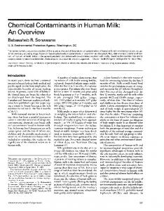
4.1. Cone constraints on λ To illustrate the use of cone constraints, we turn to an example involving the infant survival rate, and how countries may be assessed in a model that enforces specific relationship between this factor and matters of social policy. To see what is involved here, turn first to figure 6 which plots the relationship exhibited in the raw data between Y2 (infant survival rate) and X2 (share of GDP spent on government consumption net of defense and education). 1
S u 0.95 r v i 0.9 v a l 0.85
r a t e
0.8
0.75 0
0.05
0.1
0.15
0.2
0.25
Share of government expenses
Figure 6. Infant survival rates and government consumption expenditure.
B. Golany, S. Thore y Restricted best practice selection in DEA
133
Table 3 Best practice results with separate cone. Country Kenya Malawi Zambia Burma Philippines Taiwan Finland Malta Netherlands Costa Rica Argentina Guyana
θ* 0.519 0.720 0.335 0.937 0.899 1.000 0.979 1.000 1.000 0.726 0.930 0.419
Y1 0.005 0.017 – 0.001 0.022 0.015 0.057 0.027 0.063 0.018 0.009 0.025 – 0.008
Y2
Y3
Y4
X1
X2
X3
0.920 0.920 0.920 0.934 0.952 0.993 1.000 0.988 0.992 0.981 0.966 0.966
0.209 0.234 0.190 0.249 0.650 0.750 1.020 0.760 1.020 0.418 0.700 0.600
0.009 0.009 0.005 0.008 0.087 0.027 0.078 0.132 0.191 0.045 0.083 0.055
0.092 0.103 0.090 0.112 0.140 0.241 0.351 0.272 0.238 0.113 0.238 0.119
0.079 0.077 0.056 0.080 0.077 0.110 0.094 0.154 0.026 0.117 0.032 0.095
0.027 0.024 0.018 0.017 0.018 0.038 0.040 0.033 0.070 0.037 0.034 0.027
For most countries, the survival rates exceed 95% (see also column 2 in table 1). The average survival rate for all 74 countries was 95.3%. Particularly poor results were reported for Sierra Leone (82.5%) and Gambia (82.6%). To study these matters further, we first impose a rather weak separate cone constraint requiring only that the best practice survival rate must be at least 92%. The results are given in table 3. 1≥
74
∑ Y2 j ⋅ λ j ≥ 0.92.
( 24 )
j =1
As seen in table 2, three countries did not meet the 92% requirement: Kenya, Malawi and Zambia. To accommodate the new constraint, the best practice points for these countries have changed (see table 3). At the same time, their efficiency scores are pushed upwards. Clearly, since we have adjoined an additional constraint to a minimization problem, the minimal optimal value can not decrease. Turning our attention to the relationship between survival rates and net government expenditures depicted in figure 6, we make the surprising observation that increased government spending is not necessarily related to improved infant health records. If anything, the productivity of government health dollars seems to be negative. (Government spending needs to be tied to particular projects to be productive. Too often, government dollars just bolster an already bloated administration.) Insisting, nevertheless, on some weak positive relations between government health spending and survival rate, we now impose a linked cone constraint of the following nature: Starting from a hypothetical position with a survival rate of 90%
B. Golany, S. Thore y Restricted best practice selection in DEA
134
Table 4 Best practice results with linked cone constraint.
θ*
Country Kenya Malawi Zambia Burma Philippines Taiwan Finland Malta Netherlands Costa Rica Argentina Guyana
0.519 0.725 0.335 0.937 0.899 1.000 0.979 1.026 1.000 0.726 0.930 0.419
Y1 0.005 0.017 – 0.001 0.022 0.015 0.057 0.027 0.063 0.018 0.009 0.025 – 0.008
Y2
Y3
Y4
X1
X2
X3
0.911 0.927 0.916 0.934 0.952 0.993 1.000 1.000 0.992 0.981 0.966 0.966
0.200 0.235 0.190 0.249 0.650 0.750 1.020 0.774 1.020 0.418 0.700 0.600
0.007 0.009 0.005 0.008 0.087 0.027 0.078 0.132 0.191 0.045 0.083 0.055
0.092 0.104 0.089 0.112 0.140 0.241 0.351 0.276 0.238 0.113 0.238 0.119
0.061 0.077 0.056 0.080 0.077 0.110 0.094 0.150 0.026 0.117 0.032 0.095
0.023 0.024 0.018 0.017 0.018 0.038 0.040 0.033 0.070 0.037 0.034 0.027
and government spending ratio of 5%, this constraint requires an increased survival rate of at least one percentage point for each additional percentage point of government spending. The figure 1% is not important; our purpose is just to illustrate the general procedure. Mathematically,
74
−
∑ X 2 j ⋅ λ j − 0.05
j =1
74
j =1
∑ Y2 j ⋅ λ j − 0.9
≤ 0.
( 25)
The upper limit in (24) is still imposed but the lower bound is dropped. For two of the countries discussed earlier – Kenya and Malawi – this constraint is not redundant. To satisfy it, their best practice survival rates have to be increased slightly. At the same time, their efficiency ratings are adjusted upward for reasons explained above (see table 4). One additional country, Malta, has difficulties satisfying the linked cone constraint. Malta was earlier rated as efficient; now its rating is greater than one, signaling that the previous frontier point is no longer feasible. 4.2. Categorical constraints In some cases, it may be instructive to accompany the results of the original DEA model with analysis in which the comparison is restricted to a specific subgroup of the total DMU population. For instance, one may desire to run a secondary analysis in which sub-Sahara African countries are evaluated only with respect to themselves. The reason may be that the analyst feels that it is “unfair” to compare the performance
B. Golany, S. Thore y Restricted best practice selection in DEA
135
of poor or developing countries with the rich countries of the developed world. Or, it may be that one wishes to obtain an internal ranking of the Sub-Saharan countries taken by themselves. In any case, one would then set
λj = 0, j ∈{countries not in sub-Sahara}.
(26)
In our population of 74 countries, 24 were located in the sub-Sahara. Solving again, and still only exhibiting the results pertaining to the set of 12 countries presented earlier, we show in table 5 the efficiency rankings and best practice for Kenya, Malawi and Zambia. The efficiency ratings for these three sub-Saharan countries have now all improved. It is interesting to note (although it is not necessarily true in the general Table 5 Best practice results within the sub-Sahara group. Country
θ*
Y1
Y2
Y3
Y4
X1
X2
X3
Kenya Malawi Zambia
0.711 0.854 0.646
0.005 0.017 0.034
0.909 0.844 0.916
0.408 0.212 0.378
0.014 0.010 0.032
0.125 0.122 0.159
0.112 0.132 0.115
0.036 0.028 0.034
case) that the relative rankings of these three countries has not changed as their ratings improved. But, the ratings are still less than one. Thus, even with respect to the group of sub-Saharan countries, these three countries are still found to be inefficient and comparing table 1 with table 5, the specific slacks in their input-output positions can readily be identified. To illustrate the flexibility of the formulation offered in (12), we now focus our attention on the group of countries identified by Barro as “mixed economies”. Rather than excluding all other countries from consideration (as was done in (26)), we impose a weaker condition demanding that the relative weight of countries with mixed economies in evaluating one of their own should be at least 50% of the total weight sum. That is, we set UN = 0.5 in (12): ∑ j ∈N λ j ≤ 0.5, ( 27) ∑ j ∈J λ j with P being the set of mixed economies and N = J – P the other (capitalist and socialistic) economies. The figure 0.5 was chosen for illustration purposes only. The idea is simply that the comparison should mainly be carried out inside the group itself. To some limited extent, reference countries for the comparison may also be chosen from outside the group, but their combined weight should not exceed 50%. In any real application, the actual figure to be used should be selected to reflect the policy stance of the analyst.
B. Golany, S. Thore y Restricted best practice selection in DEA
136
Table 6 New best practice results for mixed economy countries. Country Philippines Argentina
θ*
Y1
Y2
Y3
Y4
X1
X2
X3
0.901 0.959
0.015 0.011
0.952 0.966
0.650 0.700
0.087 0.071
0.140 0.246
0.086 0.033
0.018 0.035
Four out of the six mixed economies displayed in tables 1 – 5 were not affected by constraint (27): Taiwan, Malta, the Netherlands and Finland. For these countries, other mixed economies already contributed at least a half of their total weight sum. However, the results for Argentina and the Philippines did change, as shown in table 6. In both cases, the original best practice (recorded in table 2) had been constructed by attaching large weights to capitalist countries such as Spain, Switzerland and Uruguay, that is, to countries outside of the group of mixed economies. Imposing (27) caused a slight improvement in the efficiency ratings for both countries. Naturally, as UN decreases, the efficiency ratings for the relevant group increase as the possible comparison possibilities decrease. The relevant facet compositions, in terms of the lambda values, with and without constraint (27), are shown in table 7. Table 7 New facet compositions for mixed economy countries. Without (27)
With (27)
Country ∑λj ( j mixed) Philippines Argentina
0.059 0.0131
∑λj (all j) 0.759 0.979
∑λj ( j mixed) 0.496 0.493
∑λj (all j) 0.992 0.987
4.3. Goal constraints We turn to a discussion of the performance of countries in terms of social and educational policy. Looking at the information provided in table 1 for countries like Kenya, Zambia and Guyana (all associated with quite low efficiency ratings), and their best practice positions as exhibited in table 2, we find significant gaps in the output variables that would have to be closed in order for these countries to become efficient. Kenya would have to increase its social security and welfare payments by more than fourfold (raising its Y4 value from 0.002 to 0.009). Zambia and Guyana would need to more than double their social security and welfare expenditures (to raise their Y4 values from 0.002 and 0.021 to 0.005 and 0.055, respectively). Realistically, one knows that it will be impossible to close these gaps in the near future. These countries seem to be locked in a severely inefficient position.
B. Golany, S. Thore y Restricted best practice selection in DEA
137
Rather than striving to achieve full efficiency, a national or international policymaking body may decide to lay down some goals of social and educational policy that reflect a more moderate ambition. While these goals should still pose a challenge, they should be attainable in light of the performance of other countries to which the country currently investigated may reasonably be compared. To illustrate the way in which DEA models can be combined with goal programming techniques, we assume that the following system of preemptive goals is given for a country currently under evaluation. First priority: The ratio of social security and welfare payments to GDP should reach 1%. That is, the goal for output Y4 is set at G4 = 0.01. To reflect the high priority of this goal, make the unit penalties for violations of these goals equal to u4+ = 0 and u4– = 9999 (see (15)). Second priority: The ratio of government expenditure on education to GDP should not fall below 3%. That is, the goal for input X3 is set at g3 = 0.03. The penalties w3+ and w3– in (15) were set to 3333 and 999, respectively. Third priority: The enrollment ratio in secondary education should reach 10% (this is a rather modest goal; only a handful of countries in the sample of 74 countries failed to reach this level). Also, the ratio of government expenditure on civilian consumption other than education, to GDP should reach at least 10%. These goals are for output Y3 and input X2 , respectively, so that G3 = 0.1 and g2 = 0.1. For the output factor we use the penalties u3+ = 0 and u3– = 999; for the input factor, the penalties w2+ = 999 and w2– = 0. The cardinal penalties mentioned here – the values 9999, 3333, 999 and 0 – are chosen so that the differences among them are large enough to assure preemption in the Goal Program. Such cardinal representations must be verified by checking that the solution generated by them have the desired properties, i.e., that a goal of a higher priority always takes precedence over lower priority goals, see, for instance, Thore [27, p. 220]. To simplify matters, the same goals were applied to all countries. Employing program (15) – (20), we obtained results as displayed in table 8 (only the social and educational variables are exhibited). Starting with the highest priority goal (on Y4), four countries originally failed to reach the targeted figure of 1%. All countries displayed in table 8 now satisfy this overriding goal. Several countries originally failed to reach the second priority goal (requiring X3 to reach 3%). Some of these countries have now reached a better best practice point that satisfies this goal, but Burma and the Philippines are still falling behind. All countries meet the third priority goal on Y3. Finally, the third priority goal on X3 poses difficulties. As most countries never satisfied this goal to begin with (see table 2), it is impossible to enforce it in most cases.
138
B. Golany, S. Thore y Restricted best practice selection in DEA
Table 8 Goal Programming solutions. Country Kenya Malawi Zambia Burma Philippines Taiwan Finland Malta Netherlands Costa Rica Argentina Guyana
5.
Y2
Y3
Y4
X2
X3
0.909 0.844 0.916 0.934 0.952 0.993 1.000 0.988 0.992 0.981 0.966 0.966
0.435 0.394 0.521 0.260 0.774 0.750 1.020 0.760 1.020 0.410 0.700 0.600
0.046 0.052 0.014 0.016 0.106 0.027 0.080 0.132 0.191 0.045 0.064 0.024
0.037 0.039 0.024 0.080 0.084 0.110 0.095 0.154 0.026 0.043 0.034 0.027
0.030 0.030 0.030 0.018 0.020 0.038 0.040 0.033 0.070 0.030 0.030 0.030
Conclusions
In this paper, we have discussed a series of situations where it might be desirable to temper the standard DEA formulations by establishing a trade-off between the conventional efficiency concept and a priori information of a different nature, such as institutional constraints, externalities in production, and considerations of fairness or equity. One of the lessons learned from a wide array of empirical work with DEA during the last decade is that the model has to be flexible. Consequently, a number of alternative DEA models have been proposed. Even so, there is often a need for customization of the model to a specific application environment. In this spirit, we have offered a variety of model extensions that increase significantly the flexibility of DEA models. Such extensions will always be bought at a price. Diluting the conventional concept of efficiency, the analysis will lose some of its discriminatory edge. Consequently, some DMUs will be accorded higher efficiency ratings than otherwise. (Mathematically, adjoining additional constraints to the minimization (1) – (4) can not cause the optimal value to decrease. Geometrically, the distance between some of the DMUs and the efficiency frontier is shortened.) While various extraneous considerations are accommodated, the meaning of the concept of efficiency becomes less clear-cut. Hopefully, we have been able to make clear in the preceding pages the mathematics of such attenuation. But it will still be up to the analyst to decide whether in a particular application at hand the advantages of the procedures outweigh their cost.
B. Golany, S. Thore y Restricted best practice selection in DEA
139
The calculations yield a new and more comprehensive metric. As a measure of productive efficiency, pure and simple, it is less sharp than the original DEA efficiency rating. Several kinds of constraint classes were identified and developed. Cone constraints, which were previously defined and used only in the multiplier side of DEA were made applicable to the envelopment side. These constraints, in either a linked or separate manner, rule out the possibility of locating a best practice point in certain areas which were otherwise feasible. Categorization constraints, which have been restricted in the literature to zero-one type decision rules (i.e., spelling out in advance whether or not a DMU can enter the basis), were here extended by defining groups of DMUs and specifying that only a certain proportion of the members in specific groups are permitted to enter the facet. The concept of “dynamic clustering” was introduced here for the first time. In contrast with “static” cones (or categorization constraints) which set identical cones for all the DMUs, in dynamic clustering a different region is fitted around each analyzed DMU, allowing other DMUs to enter its facet only if they fall within this region. Finally, we have also shown how goal programming and goal focusing may be employed to accommodate the presence of output andyor input goals. The application discussed in the text, ranking 74 countries in terms of their economic and social performance, is the most comprehensive multi-national performance evaluation done with DEA to date. While the emphasis throughout the application was on illustrating the techniques described earlier, it should be clear that a more systematic analysis of this kind might serve as a vehicle for the study of comparative economics by international agencies such as the World Bank and the UN. Finally, it should be noted that the techniques presented here are not limited to multi-national evaluation scenarios. Similar constraints, in other DEA application contexts, may be found in the operations of commercial banks regulated by a central bank [13, p. 17], electrical utilities in the presence of environmental legislation [16], and the operations of airlines in the presence of supervision by the FAA, the National Aviation Board and the Justice Department [12], etc. 5. [1] [2] [3] [4] [5]
References D.L. Adolphson, G.C. Cornia and L.C. Walters, A unified framework for classifying DEA models, in: Operational Research ’90, pp. 647 – 657. R. Banker and R. Morey, The use of categorical variables in Data Envelopment Analysis, Management Science 32(1986)1613 – 1627. R.J. Barro, Economic growth in a cross section of countries, The Quarterly Journal of Economics (1991)407 – 443. A. Charnes and W.W. Cooper, Management Models and Industrial Applications of Linear Programming, Vol. 1, Wiley, New York, 1961. A. Charnes and W.W. Cooper, Goal programming and multiple objective optimizations – Part I, European Journal of Operations Research 1(1977)39 – 54.
140
[6] [7]
[8] [9] [10] [11] [12] [12a] [13] [14] [15] [16]
[17]
[18] [19] [20] [21]
[22] [23]
[24] [25] [26]
[27]
B. Golany, S. Thore y Restricted best practice selection in DEA
A. Charnes and W.W. Cooper, Preface to topics in Data Envelopment Analysis, Annals of Operations Research 2(1985)59 – 94. A. Charnes, W.W. Cooper, B. Golany, L.M. Seiford and J. Stutz, Foundations of Data Envelopment Analysis for Pareto-Koopmans efficient empirical production functions, Journal of Econometrics 30(1985)91 – 107. A. Charnes, W.W. Cooper and E. Rhodes, Measuring efficiency of decision making units, European Journal of Operational Research 2(1978)429 – 444. A. Charnes, W.W. Cooper, J.J. Rousseau and A. Schinnar, A goal focusing approach to analysis of intergenerational transfers of income, International Journal of Systems Sciences 17(1986)433 – 446. A. Charnes, W.W. Cooper and R. Thrall, Classifying and characterizing efficiencies and inefficiencies in Data Envelopment Analysis, Operations Research Letters 5(1986)105 – 110. A. Charnes, W.W. Cooper, Q.L. Wei and Z.M. Huang, Cone-ratio Data Envelopment Analysis and multi-objective programming, International Journal of Systems Sciences 20(1989)1099 – 1118. W.W. Cooper and A. Gallegos, DEA application to Latin American airlines, IC 2 Working Paper, The University of Texas at Austin, 1992. J.D. Divine, Efficiency analysis and management of not for profit and governmentally regulated organizations, Ph.D. Dissertation, University of Texas, Austin, TX, 1986. D.D. Evanoff and P.R. Israilevich, Productive efficiency in banking, Economic Perspectives, Federal Reserve Bank of Chicago (1991) 11 – 32. M.J. Farrell, The measurement of productive efficiency, Journal of the Royal Statistical Society A20(1957)253 – 281. B. Golany, F.Y. Phillips and J.J. Rousseau, Models for improved effectiveness based on DEA efficiency results, IIE Transactions 25(1993)2 – 10. B. Golany, Y. Roll and D. Rybak, Measuring efficiency of power plants in the Israeli Electric Corporation by Data Envelopment Analysis, IEEE Transactions on Engineering Management 41, no. 3 (1994)1 – 14. B. Golany and Y. Roll, Incorporating standards in DEA, in: Data Envelopment Analysis: Theory, Methodology and Applications, A. Charnes, W.W. Cooper, A.Y. Lewin and L.M. Seiford, eds., Kluwer Academic, Boston, 1995. B. Golany and E. Tamir, Evaluation of efficiency-effectiveness-equity trade-offs: A Data Envelopment Analysis approach, Management Science 41(1995)1172 – 1184. B. Golany and S. Thore, On the treatment of negative outputs in DEA, IC 2 Working Paper, The University of Texas at Austin, 1993. B. Golany and S. Thore, The competitiveness of nations, to be published in IMPACT: How IC2 Research Affects Public Policy and Business Markets, 1995. K. Land, C.A.K. Lovell and S. Thore, Productive efficiency under capitalism and state socialism: An empirical inquiry using chance constrained Data Envelopment Analysis, Technological Forecasting and Social Change 46(1994)139 – 152. C.A.K, Lovell, Measuring the macro-economic performance of the Taiwanese economy, Research Report, The University of Georgia, Athens, GA, January 1992. C.A.K. Lovell and J.T. Pastor, Macro-economic performance of sixteen Ibero-American countries over the period 1980 – 1991, presented at the Georgia Productivity Conference, The University of Georgia, Athens, GA, October 1994. Y. Roll and B. Golany, Alternate methods for treating factor weights in DEA, OMEGA 21(1993) 99 – 109. E. Thanassoulis and R.G. Dyson, Estimating preferred target input output using Data Envelopment Analysis, European Journal of Operational Research 56(1992)80 – 97. R.G. Thompson, L.N. Langemeier, C.T. Lee, E. Lee and R.M. Thrall, The role of multiplier bounds in efficiency analysis with application to Kansas farming, Journal of Econometrics 46(1990) 93 – 108. S. Thore, Economic Logistics: The Optimization of Spatial and Sectoral Resource, Production and Distribution Systems, Quorum Books, Westport, CT, 1991.