Restructuring multi-level networks by using function approximations

Restructuring multi-level networks by using function approximations J. Cortadella

M. Kishinevsky

A. Mishchenko

Universitat Polit`ecnica de Catalunya Barcelona, Spain

SCL, Intel Corp. Hillsboro, USA

University of California Berkeley, USA

Abstract— This paper presents a technique for multi-level minimization using implicit don’t cares. One of the major problems in minimization is the calculation of the don’t care set. Conventional approaches project the global don’t cares onto the local support of each node to keep minimization cost low. This prevents restructuring multi-level networks. The approach presented in this paper enables the extension of the support for the projection of the don’t care set, while keeping a low computational complexity. The extension of the support is based on the idea of function approximations. The approach has shown to produce tangible improvements in multi-level networks when compared with existing techniques.

I. I NTRODUCTION Optimization of combinational multi-level networks is achieved by exploring flexibility of the network using logic simplification and restructuring operations. The concept of implicit (or internal) don’t cares is crucial for the node simplification. For each node ni in a network, we can use the following don’t care for simplification: DCi = EDC + SDCi + ODCi where EDC is the external don’t care and SDCi and ODCi are the satisfiability and observability don’t cares, respectively, for node ni . DCi can be represented in terms of the primary inputs of the network (global don’t cares) and projected, by image computation, on any subset of signals of the network (local don’t cares). Practical implementations of don’t care-based minimization project DCi onto the local support of the node, thus allowing the simplification of the node function and, possibly, the elimination of some signals in the support. However, the local projection of DCi never permits restructuring the network by incorporating new signals to the support of the node. Some methods, such as full simplify in SIS [1], partially lift this limitation by greadily considering a few candidate nodes whose support is a subset of the node being simplified. In other words, powerful Boolean simplification and restructuring are in large decoupled in the current methods. Restructuring techniques are typically based on adding redundant connections to some gates and then deleting a different set of redundant connections. The implementations of such techniques are typically based on ATPG [2], global flow analysis [3], transductions on the decomposed network [4], or SPFD-based rewiring [5].

In this paper we describe a method that couples simplification and restructuring together: • New potential candidates for the support of a node under minimization are computed. • Then simplification selects actual fan-in nodes based on the results of the minimization and cost function estimation. In this paper we focus on a single method for computing new fan-in candidates for the simplified node, which is based on function approximation (although other methods are possible). The basic idea is as follows: if a fan-in node, n, implements a global function, fn , that is close enough to a global function, fm , of the node m under minimization, then by incorporating n as a fan-in for m there are good chances to significantly simplify implementation of m. That is, nodes with functions that are good approximations of a minimized functions are plausible candidates to be included in the support as restructuring candidates. Using the argot of SPFDs [6], the rationale is the following: The logic function of a node distinguishes the on-set from the off-set. When optimizing the representation of the node, we rely on the distinguishing power of other nodes in the network whenever possible. By taking good approximations into the support of the node, the requirement for the node to distinguish is reduced, and as a result, the logic function of the node is simplified. A. An example Let us analyze an example of SIS optimization with the following network (inputs: a, b, c, d; outputs: x, y, z): x = ac + a c + b(c + d) y = b(ac + a c) + a bc z = a+b+d After running the SIS command full simplify, the expression for x is simplified as follows: x = y + a c + b(c + d) The simplification is possible because the SDC of node y, y ⊕ (b (a ⊕ c) + a b c)

< a, b, c, d> 15

14

13

12

11

10

9

8

7

6

5

4

3

2

1

0

x

1

1

1

0

1

1

0

0

0

0

1

1

1

1

1

1

y

0

0

0

0

1

1

0

0

0

0

1

1

1

1

0

0

z

1

1

1

1

1

1

1

1

1

1

1

1

0

1

1

0

of nodes on the critical path [7]. As our experimental resluts show (cf. V) we have managed to avoid this drawback by special provisions when selecting restructuring candidates. In particular, • •

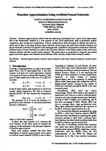
Fig. 1.

Look-up tables for nodes x, y, and z.

(a negation of the second equation) is used during the minimization of x. Considering y for simplifying x was possible, since the support of y, {a, b, c} is a subset of the support of x, {a, b, c, d}. However, this approach is not able to incorporate x or z into the fanin of y, since their support is not a subset of the support of y. Let us assume now that the support limitation is removed and we can project the DC for y onto other existing signals in the network, e.g. x. To check the effect of this with SIS we can simply “cheat” and artificially introduce x in the support of y by using a redundant form for y: y = b(ac + a c) + a bcx + a bcx After executing full simplify, the following simpler (in literal count) network is obtained: x = ac + a c + bd + z y = x(ac + b) z = a+b+d B. Using function approximation for the example Fig. 1 shows look-up tables for functions x, y, and z of the example. Let us compute the distance between the functions as a number of minterms in their boolean difference. E.g., functions x and y differs in five cells of the table (shaded boxes). The distances between all pairs of functions are: δ(x, y) = 5/16; δ(x, z) = 7/16; δ(y, z) = 10/16; δ(y, z 0 ) = 6/16 Note, that the invertion of z is closer to y, than z itself. Selecting between x and z as candidates for the support of y, we can conclude that x is better since it is closer to y (smaller distance). Moreover, x is an over-approximation of y, i.e., each time x is “1”, y is “1”. Hence, y can be implemented as an AND of y and some other function. Thus, x can be considered as a promising candidate to be incorporated in the support of y. Indeed, after minimization, the expression y = x(ac + b) is obtained. The reader can check that no improvements would be obtained when trying to include z in the support of y. Other methods of computing distances between two functions can be explored as well. Iterative restructuring techniques have good potential for area reduction at the cost of delay due to potential for sharing

There is a mode in which new candidates for the support cannot increase the logic depth of a node There is a mode restricting sharing on the new support signals that promotes tree-like structures friendly to the technology-mappers.

The numbers reported in our result tables are obtained with both modes on. The rest of the paper is organized as follows. Section II presents basics of don’t care computation. Function approximations are considered in Section III. Section IV describes methods for restructuring. Experimental results are reported abd discussed in Section V. II. I NTERNAL DON ’ T- CARES IN MUTI - LEVEL NETWORKS A. Previous Work Flexibility in the network can be captured using different techniques: don’t cares, Boolean relations, SPFDs, etc. In this paper we use don’t cares as the most widely used and computationally feasible. Both Boolean Relations and SPFDs have power to incorporate simplification and restructuring in a single framework, however Boolean Relations are too computationally expensive for even small circuits [8] and similarly SPFDs implementations [9] did not combine support restructuring with simplification so far due to the large computational cost. The well-known algorithm for don’t-care-based simplification of binary networks, developed in [10], uses a combination of satisfiability don’t-cares (SDCs) and compatible observability don’t-cares (CODCs). It was implemented as command full simplify in SIS [1]. Recently, it was shown that CODCs can be computed independently of the node’s implementation [11]. A new scheme for computing the internal don’t-cares of a node in an MV network (binary network is a particular case of MV network) is proposed in [12] and implemented in MVSIS [13]. The don’t-cares computed are complete but not compatible. Therefore, they should be used to simplify the node before any other nodes are changed. Because the don’t-cares are complete, they allow for a more thorough simplification, compared to compatible or partial don’t-cares derived by other methods, which are subsets of the complete don’t-cares [14]. Although in the past complete don’t-cares have been derived for Boolean networks where each node has a single binary output [15] or several outputs (Boolean relations) [1], they did not find practical applications until recently because of the inherent computational complexity. For network restructuring described in this paper, we use a new efficient implementation of the complete don’t-cares computation in the SIS [1] environment.

B. Terminology We assume the reader to be familiar with the concept of Boolean functions and Binary Decision Diagrams [16]. Definition 2.1: The Boolean function of a node (completely or incompletely specified) expressed in terms of the node’s inputs is the local function of the node. The same function expressed in terms of the primary inputs (PIs) of the network is the global function of the node. The node function can also be expressed in terms of any set S of variables of the network (not necessarily fanins of the node or PIs of the network). This representation is called the projection of the node’s function onto S. The global functions are computed by visiting all nodes of the network in a topological order from the PIs to the PIs. The global functions of the PIs are set to be equal to the elementary variables. When a node is visited, the global functions of the fanins are already computed. To compute the global function of the node, its local function is composed with the global functions of the fanin nodes. The projection of the node’s function onto an arbitrary subset of nodes in the network can be computed by the image computation [17]. C. Don’t-cares The external don’t-cares (EXDCs) for a primary output (PO) expresses the condition when the PO can take any value. Besides EXDCs, the sources of don’t-cares at a node are the limited satisfiability and observability of the node, illustrated in Example 2.1 and Example 2.2, respectively. Example 2.1: Let N be the network containing node n. Let x and y be fanins of n, expressed in terms of PIs of the network, a and b, as follows: x=a ∨ b

y = a ∧ b.

It is easy to see that the combination (x = 0, y = 1) is never realized at the inputs of node n. This combination is an example of a local satsfiability don’t-care of node n, because it is expressed using the fanin variables of node n. Example 2.2: Let N be the network containing node n. Let node n have exactly two fanouts, u and v, specified using formulas: u=n ∨ a v=n ∨ b where a and b are the PIs of the network. It is easy to see that combination (a = 1, b = 1) makes the output of node n immaterial because it never reaches the POs. This combination is an example of a global observability don’t-care of node n, because it is expressed using the PIs of the network. Flexibility can be measured by the number of don’t-care minterms in the corresponding ISF. The larger the don’tcares, the more freedom is available to optimize the node. For practical applications, it is important to have efficient don’tcare computation procedures, e.g., similar to the one described below. Definition 2.2: The don’t-cares are complete if it is not possible to add another don’t-care minterm, without affecting the functionality of the network.

D. Don’t-care computation The following definition is required to describe the procedure for computing different representations of the complete don’t-cares of a node in the network. Definition 2.3: For a given node n, the cut (at n) network is obtained from the original network by replacing n in the local functions of the n’s fanout nodes by an additional PI of the network. The cut network is a model used to detect the influence of the node on the global functions of the network. The actual representation of the original network is not modified when the cut network is used in the computation. Theorem 2.1 (Global Don’t-Care Computation [12]): Let the global functions and EXDCs of the POs of the network be, respectively, Fi (X) and DCi (X), where i is the index of a primary output, and X is the set of PIs. Let the global function of the POs of the cut network be Fi (X, z), where z is the additional PI representing a node. The complete global don’t-cares of node z are computed as follows: ^ DCz (X) = ∀z [(Fi (X) ⊕ Fi (X, z)) =⇒ EXDCi (X)] i

Interpretation. The global don’t-cares for the node is derived assuming that, for all output values of the node and all outputs of the network, the difference between the global function of the original network and global function of the cut network (Fi (X) ⊕ Fi (X, z)) is contained ( =⇒ ) in the EXDCs. If there are no EXDCs, this formula requires that there were no difference between the global functions. The next Theorem extends the local don’t care computation from [12] in that the latter uses only the mapping of PIs into the local variables of the node, while the former allows for an arbitrary mapping. Theorem 2.2 (Projected Don’t-Care Computation): Let z be a node with the global don’t-care function DCz (X). Let X be the set of PIs and S = {yj } be an arbitrary subset of nodes with the global functions, Yj (X). Then, the don’t-cares of node z projected onto S are computed as follows: DCz (Y ) = ∀X [MS (X, Y ) =⇒ DCz (X)]

(1)

where MS (X, Y ) =

^

[yj ≡ Yj (X)] .

j

Interpretation. The expression MS (X, Y ) is the transition relation [17], which defines the mapping between the PIs, X, and the variables from the set S. The projected don’tcares are computed assuming that, for all PI minterms, either the mapping is false, MS (X, Y ) = 0, or the global don’tcare is true, DCz (X) = 1. When the mapping is false, the corresponding local minterms cannot be produced under any assignment of the PIs. This corresponds to the satisfiability don’t-care of the node. When the global don’t care is true, it means that the given assignment of PIs is in the scope of external and observability don’t-cares. Taking all types of don’t-cares into account, this formula derives the complete don’t-care of the node z projected on set S.

h=−

III. F UNCTION APPROXIMATIONS The proposed selection of nodes to participate in the support of other nodes is based on the concept of function approximation. We first present some definitions required in this section. Definition 3.1 (Satisfying fraction): Given a Boolean function f , the satisfying fraction of f , denoted by |f |, is the fraction of assignments that satisfy f . The satisfying fraction is a value in the interval [0, 1]. As examples, the functions f = a, g = ab and h = a + b, have satisfying fractions of |f | = 1/2, |g| = 1/4 and |h| = 3/4. The satisfying fraction can be recursively calculated as follows:  if f = 1  1 0 if f = 0 |f | =  |fa |+|fa | otherwise 2 This definition suggests a linear-time calculation of |f | when f is represented as a BDD. Definition 3.2 (Distance between two functions): The distance between two Boolean functions f and g, denoted by δ ∗ (f, g), is the fraction of assignments x, such that f (x) 6= g(x). The distance between two functions can be calculated as δ ∗ (f, g) = |f ⊕ g| Usually, we are interested in the distance between f and g, or the complement of any of them. Thus, the concept of distance is extended as follows: δ(f, g) = min(δ ∗ (f, g), δ ∗ (f, g)) The following statements are easy to prove: δ ∗ (f, g) = δ ∗ (f , g) ∈ [0, 1] δ ∗ (f, g) = δ ∗ (f , g) = 1 − δ ∗ (f, g) δ(f, g) ∈ [0, 1/2] Distance is a measure of similarity between functions. If f = g or f = g, then the distance between both functions is 0. The reader will not find difficult to prove that the distance between two functions that have disjoint support is always 1/2. Definition 3.3 (Over- and under-approximations): f is said to be an over-approximation of g if g =⇒ f . In this case, g is said to be an under-approximation of f . In this paper, we are interested in the minimization of Boolean networks. When doing so, using the flexibility provided by the don’t-care space of the network is crucial. The concepts presented so far can be extended when a don’t-care space is considered. Definition 3.4 (Extensions with don’t-cares): The previous definitions can be extended when a don’t-care space, represented by a Boolean function d, is considered. The extensions are as follows: δ ∗ (f, g, d) = |(f ⊕ g) · d| δ(f, g, d) = min(δ ∗ (f, g, d), δ ∗ (f, g, d)) and f is an over-approximation of g (or g an underapproximation of f ) if g · d =⇒ f .

h=1

f

h=0

f

g (a)

Fig. 2.

h=−1 h= 1− −1 h=00

h=−0

g

(b)

Minimization with function approximations.

For simplicity, we will omit the argument d when it is implicit from the context. We say that a function f is a good approximation of another function g when the distance between them is small. We will next show that good approximations are promising candidates to participate in the support of a function under minimization. This is the basis of the restructuring approach presented in this paper. Even though it can be argued that the size of the don’tcare is not always a good indication of the flexibility to minimize a Boolean function, it is reasonable to assume that the minimization with a larger don’t-care space tends to deliver better results, in general. The heuristics presented in this paper are based on this arguable fact. The results corroborate that the heuristics are useful to minimize Boolean networks. A. Minimization with over- and under-approximations Let us start with a simple example. Assume that f and g are nodes of a Boolean network and g is an over-approximation of f (see Fig. 2(a)). Thus, g can be a Boolean factor of f such that f =g·h where h can be defined as an incompletely specified function as follows: hon = f ; hoff = f · g; hdc = g If we measure the flexibility to minimize h as the size of its don’t-care set, we have that |hdc | = |g|. In other words, |hdc | becomes larger when δ ∗ (f, g) becomes smaller. Note that, in the ideal case in which δ ∗ (f, g) = 0, we have that hoff = 0 and the trivial implementation h = 1 is valid. This indicates that f and g are equivalent and f can be substituted by g in the Boolean network. The previous reasoning can be done when g is an underapproximation, with f =g+h and hon = f · g; hof f = f ; hdc = g with |hdc | = |g|. Finally, the extension for the case in which a don’t-care space exists is straightforward.

B. Minimization with general approximations Let us assume now that g is neither an over- nor an underapproximation of f . Thus, g can be a Boolean divisor of f according to the following expression1 f = g · h1 + h2 .

f 0 0 1 1

g 0 1 0 1

h1 – 0 – 1 –

h2 0 0 1 – 1

In this case, the similarity between f and g determines the flexibility for h = (h1 , h2 ). In order to increase the flexibility we need to: • reduce the region R01 , thus moving assignments to the region R00 and increasing the flexibility for h1 , or • reduce the region R10 , thus moving assignments to the region R11 and increasing the flexibility for h2 . Ideally, we would like to have f = g, thus allowing h1 = 1 and h2 = 0 be constant functions. In general we would like g to be a good approximation of f . The approximation-based minimization can be also studied from the point of view of SPFDs [6], [9]. Each function f must perform an effort to distinguish the on-set from the off -set vertices. The support of the function provides enough information to do that, and the function combines that information to produce the result. If one of the inputs in the support, say g, is a good approximation of the function, it means that g has already performed a significant effort to distinguish the on-set from the off -set of f . Thus, the effort left for f is small and the complexity of the function can be low. IV. A LGORITHMS The main contribution of this paper is the selection of the set of nodes S in equation 1 for the calculation of the local don’t-cares. By defining S to include nodes that are not in the local fanin, the possibility or restructuring is introduced. Two complementary approaches for restructuring are presented. The first one aims at reducing the complexity of each node individually. The second one attempts to eliminate nodes that can be substituted by other nodes. In both approaches, the selection of candidates for restructuring a node is identical. A. Selection of restructuring candidates The set of candidates S to minimize a node n includes nodes from four different categories. The order of the categories is 1A

LF SS OA

The flexibility for minimization is now distributed between h1 and h2 and can be specified as a Boolean relation as shown in the following table (see Fig. 2(b)): Region R00 R01 R10 R11

important since, for each category, only those candidates not included in the previous categories are eligible.

division as (g + h1 ) · h2 is also possible, leading to similar conclusions.

GA

(local fanin): the nodes in the local fanin of n. (same support): nodes whose local fanin is a subset of the local fanin of n. (over-approximation): nodes not in SS that are overor under-approximations of n. (general approximation): nodes not in SS that are general approximations of n.

The calculation of approximations is done by using the global functions of the nodes and the global don’t care of n. Note that the previous categories define a partition of the network since any node is a general approximation of another one. The nodes in the transitive fanout of n are excluded from the sets SS, OA and GA. Otherwise, combinational cycles would be created in case they would be selected for restructuring. After having classified all nodes, the best approximations are selected for each of the categories SS, OA and GA. In particular, the selection is tuned by three parameters KSS , KOA and KGA that indicate how many nodes must be chosen within each category. The selected nodes are those with the smallest value of δ(m, n, DCn ) calculated in the global space.

B. Local restructuring The approach used for local restructuring is identical to the one used for multi-level minimization, with the exception that the set S for the calculation of local don’t-cares is extended with approximate candidates, as previously described. In our case, we use as a basis the approach presented in [12] restricted to binary multi-level networks.

C. Global restructuring The minimization of each node is typically done by a twolevel minimizer that aims at reducing the number of literals of a cover. With a greedy approach, restructuring would never be produced if that involves increasing the number of literals of an individual node. However, increasing the complexity of a node may have a positive influence in the rest of the network if some other nodes can be simplified or eliminated. We say that a node n1 is a dominator of another node n2 if n1 belongs to all paths from n2 to any primary output. We also say that n2 is dominated by n1 . The strategy for global restructuring aims at eliminating nodes with single fanout and the nodes dominated by them (see Fig. 3). Thus, for each arc m → n in the network such that n is the only fanout of m, the following procedure is executed:

m

n

(a)

m

n’

(b)

Fig. 3.

Algorithm full simplify mfs mfs -r fsapp

Before Mapping Levels Fact. Lit. CPU 240 7543 3.50 247 7457 5.30 236 11841 4.10 218 7320 19.50

After Mapping Delay Cell Area 273.26 4865504 277.58 4884528 262.83 7488960 240.02 4757392

TABLE I C OMPARING STANDALONE APPLICATION OF full simplify, mfs, AND fsapp.

Multi-level restructuring.

S := candidates for minimizing n; dc := DCn (S); {calculation of the local DC with S} on := “local function of n” · dc; {local on-set with S} off := on + dc; {exclude m from the support and check whether it is essential} (on, off , dc) := (∃m on, ∃m off , ∀m dc); if on ∩ off = ∅ then { m is not essential } n0 := minimize (on, off , dc); D := {m} ∪ set of nodes dominated by m if n would be substituted by n0 ; if lits(n0 ) - lits(n) ≤ lits(D) then Substitute n by n0 ; Remove nodes in D; endif endif

Initially, the ISF for n using the extended support S is calculated. Next, m is excluded from the ISF by performing the exsitential abstraction in the on- and off -set, and the universal abstraction in the dc-set. The variable is not essential if the on- and off -set do not intersect after the abstractions. Next, the cost of substituting n by n0 , in which m is not present, is calculated. In case the increased cost is compensated by the removal of m and the dominated nodes, the restructuring is accepted. The nodes dominated by m are shadowed in Fig. 3. It is important to realize that some of the nodes dominated by m before restructuring (shadowed nodes in Fig. 3(a)), may not be dominated after restructuring (see Fig. 3(b)). V. R ESULTS The method for multi-level combinational logic optimization presented in this paper has been implemented as a fsapp command in SIS. The primary goal of the experiments was to compare the new method with • a classical full simplify command that uses the satisfiability and compatible observability don’t cares and • an mfs command that uses roughly the same strategy as full simplify, but with complete don’t cares (as explained in section II-A). Our fsapp has two modes of operation corresponding to the global and local restructuring as explained in Sections IVC and IV-B. The comparison strategy is to call fsapp for one iteration of global restructuring followed by an iteration of local restructuring in place of a call to full simplify or mfs, correspondingly. The quality of results was evaluated after technology mapping using the map -n1 -AFG command of SIS and the lib2.genlib library. We also confirmed consistency of the results using another technology mapper

Script sweep rugged mfs mfs -r fsapp

Levels 794 831 838 835 808

Before Mapping Fact. Lit. CPU 111007 0.60 45521 4317.30 46979 245.90 49238 241.00 39604 871.60

Delay 862.22 946.84 955.27 950.87 915.62

After Mapping Cell Area 69422752 30850432 31607680 33182960 26806208

TABLE II C OMPARING APPLICATION OF full simplify, mfs, INSIDE script.rugged.

AND

Gates 46496 21716 22153 23281 18917

fsapp

and another library available to us. The experiments have been run on 69 circuits from the IWLS’91 benchmark set of multilevel combinational circuits [18] and its smaller subset of 34 circuits (for fast comparison). First we compared the three methods taken standalone, i.e., by running the commands under comparison after the sweep on the original circuits from a subset of 34 circuits. Table I illustrates the comparison results. fsapp obtains an overall reduction of 12% in delay and 2% in area comparing to full simplify and a bit larger reduction comparing to the mfs. The third line of the table corresponds to the application of mfs with no restructuring, i.e. when support of the node cannot be changed by incorporating other nodes from the “same support” category. The results in this case are much worse in area than the default mfs. The second set of experiments compared fsapp, full simplify, and mfs within the rugged script, a popular SIS script that uses full simplify. We replaced full simplify inside rugged with mfs and fsapp, correspondingly. A larger set of 69 circuits was used for this comparison. The results are presented in Table II. The first line gives as a reference the resulting numbers for the original circuits (after sweep), the second line is for the script.rugged. A large run time for the script.rugged is primarily due to one example, too large. Overall, we can conclude that even after significant amount of optimization by the ealier commands of script.rugged, fsapp could deliver about 13% area reduction simultaneously with 3% delay reduction (after technology mapping) as compared with the rugged and even bigger delay and area reduction comparing with the mfs. Table III gives comparison on the individual examples between the script.rugged (the right part of the table) and it’s version with fsapp (the left part of the table). Only

example alu4 apex6 apex7 b1 b9 C17 C1908 C2670 C3540 C432 C5315 c8 cc cm151a cm162a cm85a comp cordic cu frg1 frg2 i10 i1 i3 i8 i9 lal pair pm1 rot t481 term1 ttt2 x1 x3 x4 alu2 9symml too large

PI 14 135 49 3 41 5 33 233 50 36 178 28 21 12 14 11 32 23 14 28 143 257 25 132 133 88 26 173 16 135 16 34 24 51 135 94 10 9 38

PO 8 99 37 4 21 2 25 140 22 7 123 18 20 2 5 3 3 2 11 3 139 224 16 6 81 63 19 137 13 107 1 10 21 35 99 71 6 1 3

LIT 1293 1288 384 16 198 13 798 1281 2551 409 2883 239 82 53 76 81 170 118 94 383 1269 4123 71 256 2111 1050 171 2931 71 1207 210 377 371 628 1380 602 743 442 918

DPTH 27.0 14.0 11.0 3.0 7.0 3.0 27.0 28.0 35.0 33.0 27.0 7.0 4.0 7.0 7.0 6.0 9.0 8.0 6.0 9.0 15.0 32.0 7.0 5.0 10.0 9.0 6.0 23.0 7.0 16.0 10.0 9.0 10.0 7.0 12.0 11.0 20.0 12.0 11.0

rugged with GATE 579 569 206 7 106 7 412 612 1221 255 1129 110 52 19 41 37 99 54 46 164 618 1891 45 178 864 402 88 1246 40 570 142 174 167 284 608 358 363 203 403

fsapp AREA 840304 825456 279328 10208 145232 9280 567472 859792 1732576 333152 1710304 157760 68208 30624 54752 52896 131776 77488 64960 242208 863968 2710224 58000 223648 1300128 628720 122032 1835120 52432 807360 181424 248704 238960 409248 882992 470032 512256 293712 589280

DELAY 30.63 15.55 11.82 3.85 7.71 3.04 31.55 27.24 37.22 33.80 27.55 8.47 6.53 5.86 6.80 6.96 10.31 6.95 8.67 11.83 19.66 38.84 7.37 4.60 15.10 12.77 7.29 24.42 9.58 19.42 11.33 9.97 12.57 8.56 13.23 10.62 24.10 14.90 13.88

LIT 1256 1344 402 17 265 14 810 1512 3900 561 2950 238 84 55 102 84 174 134 95 390 1352 6064 74 620 2132 1054 179 3062 75 1376 1362 371 408 642 1534 628 668 432 758

rugged classic (with DPTH GATE 26.0 623 14.0 599 12.0 223 4.0 10 8.0 129 3.0 10 27.0 424 28.0 704 36.0 1747 32.0 283 28.0 1190 7.0 112 5.0 55 6.0 25 8.0 54 7.0 41 10.0 103 9.0 57 6.0 48 10.0 166 14.0 679 35.0 2729 8.0 47 7.0 306 10.0 917 9.0 567 7.0 94 27.0 1326 7.0 44 16.0 651 15.0 662 9.0 170 10.0 187 7.0 287 12.0 608 10.0 355 22.0 341 12.0 192 12.0 353

full simplify) AREA DELAY 873712 30.89 868608 15.76 301600 11.73 13456 4.30 180960 8.35 12528 3.58 582320 31.36 999920 28.61 2538544 40.68 396720 35.72 1783152 28.22 159616 8.29 71456 6.29 36656 6.25 73776 8.15 58000 8.04 135952 11.82 83984 7.60 67280 8.61 245920 12.06 942848 17.42 3944000 45.84 60784 7.36 427808 6.37 1355808 14.91 782304 13.19 128992 9.03 1953440 28.35 58464 9.12 925216 21.62 932640 16.95 245456 10.41 268656 13.79 415744 9.01 927536 13.24 476992 10.58 475136 23.80 282576 13.90 507616 13.58

TABLE III C OMPARING script.rugged WITH fsapp AGAINST script.rugged ON INDIVIDUAL EXAMPLES .

selected examples for which there was a significant difference in results are shown. On other examples the results have been identical or close. The top (large) part of the table shows examples for which fsapp performed better, while the bottom part - three examples on which the classic script was superior. The columns from left to right shows the name of the example, number of primary inputs and outputs, and then the number of literals in the multi-level network, the depth of the technology-independent network, the gate count, area and delay after technology mapping for the fsapp and the classic rugged, correspondingly. Note that for some of the examples rugged with fsapp could get a dramatic improvement (all optimization results are verified by the equivalence checking). E.g., in case of t481 the fsapp achieved more than 5x area reduction with the simultaneous 33% reduction in delay. We could not get anywhere close to this result with other existing SIS scripts. Table IV shows how often local and global restructuring have been used for some of the examples. The top part of the table reports numbers for the local node restructuring. Only

examples for which more than ten nodes have been changed by fsapp are shown. The top part of the table ends with a line LTotal that lists numbers for all the examples. The bottom part of the table reports numbers for global restructuring on some of the example (with more than one node changed) and summarizes overall numbers in the line GTotal. The columns from left to right reports the following statistics. • The number of changed nodes, Ch, e.g. alu4 has 27 nodes changed. • The number of restructured nodes, Res, i.e. changed nodes with new fan-ins due to changes in the support of the node. alu4 has 19 restructured nodes. • The number of restructuring inputs, rIn, further partitioned into three categories: SS, for the same support, OA for over- and under-approximations, and GA for general approximations. E.g. if restructuring of a node involved the incorporation of three new fan-in nodes, two of which have the subset of the support for the current node, and one is a general approximation, then these new fan-in nodes will be counted in each corresponding category.

example alu4 apex6 apex7 C1908 C2670 C3540 C432 C5315 comp frg2 i10 i8 pair rot t481 term1 ttt2 x3 x4 LTotal C3540 C5315 i10 rot t481 GTotal

nodes Ch Res 27 19 22 9 15 8 11 3 19 2 43 19 25 10 27 18 16 0 50 32 105 43 16 11 85 24 31 15 167 12 13 3 16 9 23 13 12 6 820 307 2 2 2 2 7 5 2 2 7 6 30 23

new inputs rIn SS OA GA 35 11 9 15 11 5 0 6 8 4 1 3 5 2 0 3 5 4 0 1 25 9 0 16 16 1 0 15 28 15 2 11 0 0 0 0 61 51 1 9 56 35 5 16 15 8 2 5 39 35 1 3 19 18 0 1 14 4 5 5 3 1 1 1 18 10 1 7 18 11 1 6 7 2 1 4 465 275 37 153 3 1 0 2 4 2 0 2 13 8 1 4 2 2 0 0 14 5 0 9 53 27 1 25

nodes with k new inputs 0 1 2 >2 8 12 2 5 13 7 2 0 7 8 0 0 8 1 2 0 17 0 1 1 24 14 4 1 15 4 6 0 9 10 6 2 16 0 0 0 18 4 27 1 62 32 10 1 5 7 4 0 61 10 13 1 16 12 2 1 155 10 2 0 10 3 0 0 7 2 5 2 10 9 3 1 6 5 1 0 513 180 102 25 0 1 1 0 0 0 2 0 2 1 2 2 0 2 0 0 1 2 1 3 7 7 8 8

in TFI? TFI nTFI 22 13 4 7 1 7 5 0 3 2 13 12 16 0 4 24 0 0 9 52 28 28 6 9 9 30 13 6 4 10 1 2 5 13 8 10 1 6 184 281 3 0 3 1 11 2 1 1 12 2 43 10

TABLE IV S TATISTICS FOR LOCAL ( THE TOP PART ) AND GLOBAL ( THE BOTTOM PART ) RESTRUCTURING ON THE SELECTED EXAMPLES .

alu4 has 35 restructuring inputs, 11 of which are from the same support, 9 are over/under approximations, and 15 are general approximations. • The next four columns reports statistic relating changes of the nodes with the number of new inputs incorporated: k = 0 - how many nodes were changed without incorporating any new input, equivalent to Ch-Res (8 for alu4), k = 1 - number of nodes changed incorporating 1 new input (12), k = 2 - number of nodes changed incorporating 2 new inputs (2), and k > 2 - number of nodes changed incorporating more than 2 inputs (5). • The last two columns indicate that for the alu4 from the 35 new inputs that were incorporated in changed nodes, 22 were in the transitive fanin of a node under minimization (TFI column) and 13 were out of the transitive fanin (nTFI column). This table indicates that fsapp restructuring may lead to a significant area or/and delay optimization. E.g. for the t481 global restructuring of 6 nodes and local restructuring of 12 nodes further led to changes in 156 other nodes. We can conclude that restructuring of multi-level networks based on changing node support is a powerful tool for optimizing area and delay. We have demonstrated that function approximations is a good method for selecting candidates for such restructuring. We have explored a few methods for function approximations and plan to do a more careful investigation of the approximation metrics and methods in the future. VI. C ONCLUSIONS This paper presented a method combining multi-level network simplification based on complete don’t cares with re-

structuring based on support extension using function approximations. The results demonstrates that typically we can get significant area reduction without compromising (or improving) the delay as compared to the known methods of multilevel simplification. A few avenues can be explored to further improve the results: • different methods of function approximation, • using layout-oriented measures for restructuring, • this approach provides a logic synthesis framework for generating of constructive cyclic circuits,which can improve area or delay. This is an interesting (although not practical since no or little tools in the design flow support combinational cycles) research topic. R EFERENCES [1] E. M. Sentovich, K. J. Singh, L. Lavagno, C. Moon, R. Murgai, A. Saldanha, H. Savoj, P. R. Stephan, R. K. Brayton, and A. SangiovanniVincentelli, “SIS: A system for sequential circuit synthesis,” U.C. Berkeley, Tech. Rep., May 1992. [2] S.-C. Chang and M. Marek-Sadowska, “Perturb and simplify: multilevel boolean network optimizer,” IEEE Transactions on ComputerAided Design, vol. 15, no. 12, pp. 1494–1504, Dec. 1996. [3] C. L. Berman and L. H. Trevillyan, “Global flow optimization in automatic logic design,” IEEE Transactions on Computer-Aided Design, vol. 10, no. 5, pp. 557–564, May 1991. [4] Y. Matsunaga and M. Fujita, “Multi-level logic optimization using binary decision diagrams,” in Proc. International Conf. Computer-Aided Design (ICCAD), 1989, pp. 556–559. [5] J. Cong, Y. Lin, and W. Long, “SPFD-based global rewiring,” in International Symposium on Field Programmable Gate Arrays (FPGA), Feb. 2002, pp. 77–84. [6] S. Yamashita, H. Sawada, and A. Nagoya, “A new method to express functional permissibilities for LUT-based FPGAs and its applications,” in Proc. International Conf. Computer-Aided Design (ICCAD), 1996, pp. 254–261. [7] R. Rudell, “Tutorial: Design of a logic synthesis system,” in Proc. ACM/IEEE Design Automation Conference, 1996, pp. 191–196. [8] Y.Watanabe and R. Brayton, “Heuristic minimization of multiple-valued relations,” IEEE Transactions on Computer-Aided Design, vol. 12, no. 10, pp. 1458–1472, October 1993. [9] S. Sinha and R. K. Brayton, “Implementation and use of spfds,” in Proc. International Conf. Computer-Aided Design (ICCAD), 1998, pp. 103– 110. [10] H. Savoj and R. Brayton, “The use of observability and external don’tcares for the simplification of multi-level networks,” in Proc. ACM/IEEE Design Automation Conference, 1990, pp. 297–301. [11] R. Brayton, “Compatible observability don’t-cares revisited,” in Proc. International Workshop on Logic Synthesis, 2001, pp. 121–126. [12] A. Mishchenko and R. Brayton, “Simplification of non-deterministic multi-valued networks,” in Proc. International Conf. Computer-Aided Design (ICCAD), 2002, pp. 557–562. [13] MVSIS Group, “MVSIS,” UC Berkeley, www-cad.eecs.berkeley.edu/mvsis. [14] A. Mishchenko, “An experimental evaluation of algorithms for computation of internal don’t-cares in Boolean networks,” Portland State University, Dept. ECE, Tech. Rep., Sept. 2001, www.ee.pdx.edu/˜alanmi/research/net/DCcomparison.pdf. [15] H. Savoj, “Don’t cares in multi-level network optimization,” Ph.D. dissertation, UC Berkeley, May 1992. [16] R. Bryant, “Graph-based algorithms for boolean function manipulation,” IEEE Transactions on Computers, vol. C-35, no. 8, pp. 677–691, Aug. 1986. [17] H. Touati, H. Savoj, B. Lin, R. Brayton, and A. SangiovannniVincentelli, “State enumeration of finite state machines using BDDs,” in Proc. International Conf. Computer-Aided Design (ICCAD), 1990, pp. 130–133. [18] IWLS’91 benchmark set, http://www.cbl.ncsu.edu/CBL Docs/lgs91.html.