17-21 Nov. 2007 Luxor, Egypt ... nonlinear functions[3], they are the most popular artificial neural networks structures for generating many input-output nonlinear ...
6th Conference on Nuclear and Particle Physics 17-21 Nov. 2007 Luxor, Egypt
FUNCTION APPROXIMATION OF TASKS BY NEURAL NETWORKS L. Ait Gougam, A. Chikhi and F. Mekideche-Chafa Laboratoire de Physique Théorique , Faculté de Physique, USTHB BP 32, El Alia, Bab Ezzouar, Alger, Algérie Abstract For several years now, neural network models have enjoyed wide popularity, being applied to problems of regression, classification and time series analysis. Neural networks have been recently seen as attractive tools for developing efficient solutions for many real world problems in function approximation. The latter is a very important task in environments where computation has to be based on extracting information from data samples in real world processes. In a previous contribution, we have used a well known simplified architecture to show that it provides a reasonably efficient, practical and robust, multi-frequency analysis. We have investigated the universal approximation theory of neural networks whose transfer functions are: sigmoids (because of biological relevance), Gaussian and two specified families of wavelets. The latter have been found to be more appropriate to use. The aim of the present contribution is therefore to use a "mexican hat wavelet" as transfer function to approximate different tasks relevant and inherent to various applications in physics. The results complement and provide new insights into previously published results on this problem Keywords: Function Approximation, Neural Networks, Wavelets, Tasks. I - INTRODUCTION Function approximation is a central task in numerous engineering applications ranging from dynamic system identification to control, fault detection and isolation, optimization and classification[1],[2]. It refers to fitting equations (i.e., function approximators) to observed data. In the literature, the term function approximator is used to represent multivariable approximation models, mostly nonlinear, which possess a number of adjustable parameters known as weights. Feedforward neural networks are known to be universal approximators of nonlinear functions[3], they are the most popular artificial neural networks structures for generating many input-output nonlinear mappings. The training and optimization of neural networks to perform tasks involving function approximation is well documented in the literature [1],[2],[8],[9]. In applications, the main design objective is often to find a network which is a good approximator to some desired input-output mapping. However, in addition to the conventional notion of approximation, neural networks are valued especially for their ability to generalize, i.e., to use information they have learned in order to synthesize similar but non identical
-443-
input-output mappings under novel circumstances. The combination of neural networks and wavelets give rise to an interesting and powerful technique for function approximation. In the present work, three transfer functions will be first tested, viz., a sigmoidal function [6], a Gaussian one[7], and two wavelets[5]. We will then investigate the universal approximation theory of neural networks applied to different tasks relevant and inherent to various applications in physics. A well known simplified architecture [4] is used to show that it provides a reasonably efficient, practical and robust, multifrequency analysis. The training algorithm used consists on optimizing the task with respect to first, the output weights ωi and second, to the scale parameters λi. The paper is organized as follows. The model with the main basis functions is briefly described in section II, followed by the architecture of the network in section III. Section IV is concerned with the learning algorithm. Numerical results are presented in section V and finally some conclusions are drawn.
II – MAIN BASIS FUNCTIONS In the language of function approximation theory such an approximation scheme is termed discrete linear approximation, since an unknown function F: is approximated by a function Fm being a linear span of a set of m basis functions fk(·): RN→R, k=1,2,...,m. This type of mapping is given by
Fm ( X ) =
m
∑ ω k f k ( X ) + ω0
(1)
k =1
For such a network the approximation task consists of the following steps:
{
}
P
i. Provide samples ( xi , yi ) ∈ R N × R , i.e., P training pairs of an unknown function y i =1 belonging to some normed space of functions Y, ii. Define a family Φ of basis functions f k ∈ φ . iii. Use appropriate number of m basis functions from family Φ and find a corresponding set of weights ωk , k=1,2,...,m so that the error ε = F − Fm i.e., the distance ε, according to a norm
.
, (e.g., Euclidean) between an unknown function F and its estimate Fm falls
within an acceptable margin. In step (ii) of the algorithm, the family of basis functions is predetermined (i.e., the type of basis functions and their number). These basis functions (also refereed to as activation or transfer functions) can be chosen from a variety of functions such as sigmoidal functions, polynomials, trigonometric functions, exponential functions, orthogonal or non-orthogonal functions and radial functions, to mention just a few. In many situations, the appropriate choice of the basis functions plays a crucial role in the quality and control of the approximation. Function approximation based on wavelets[5] have been recently attracted the attention of many researchers as a very good alternative to more classical techniques. They constitute a class of functions that satisfy a set of important mathematical properties. A wavelet is a function ψ ∈ L2 ( R ) with zero average that satisfies certain admissibility conditions
(e.g.,
sufficient
decay
of
-444-
its
modulus).
A
family
of
functionsψ a ,b ( x ) = waveletψ 1,0 .
1 ⎛ x−b⎞ ψ⎜ ⎟ can be obtained by translating and dilating a prototype a ⎝ a ⎠
III – NETWORK ARCHITECTURE Before proceeding further, it is well to give an outline of the model and the architecture of the neural network. Consider an input X which must be processed into an output (a task) F(X). Consider now neural elementary units which receive the same input X. Each unit returns an output f which depends on two parameters: the translation parameter b and the scale one λ. Output synaptic weights ω(b,λ) linearly regroup these elementary outputs into a global output F(X). We have then the expansion [5]
F(X) = ∫ dbd λω (b, λ ) f((X − b)/λ)
(2)
Discretizing Eq.(2) with N units and neglecting the translation parameter b, we obtain the following approximation function[4] N
Fapp ( X ) = ∑ ω (λi ) f ( X / λi )
(3)
i =1
where we have used a seemingly poorer but simpler expansion which does not use the second parameter b. The central issue of any theory of neural nets is to find the values of the synaptic weights ωi which are best suited for a given task.
IV – LEARNING ALGORITHM To define the "best" Fapp, one has to minimize the square norm of the error F-Fapp. First in terms of the synaptic weights ωi and second in terms of a parameter λ. For this, we minimize the square norm of the error ε given by
ε = F − Fapp F − Fapp
(4)
in terms of ωi and in terms of λi. We obtain the two equations [3]
ωi = 2ω j
λ j2
N
∑ ( g −1)ij j =1
f j F , i = 1,..., N
Xf '( X / λ j ) F − Fapp = 0, j = 1,..., N
-445-
(5)
(6)
where g is the matrix with elements g jk = f j f k
and f’ the derivative of the elementary
task.
V – SIMULATION RESULTS Consider the target task, given by F(X) = 0.10167 exp(-x/10) {0.60717 tanh [4(x-1.66133) ] - 4.33575 tanh [4(x-9.56591)]} (7) We start the learning process by minimizing the square norm of the error in terms of the synaptic weightsωi, by satisfying equation (5). Let us take N=5 and start with the initial values 1/4, 1/2, 1, 2 and 4 for the λi 's. We then use the values of ωi to find the new values of 2
the scale parameters minimizing the error. After about 80 steps, a saturation of Fapp occurs and a close comparison between F and Fapp can be provided. Before proceeding further, it is worth noticing that all our runs converge reasonably smoothly to a saturation of the norm of 2
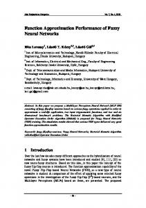
Fapp . Figure 1 illustrates the results obtained in the case sigmoids [f(x ) = (1/(1+exp (-x)))]
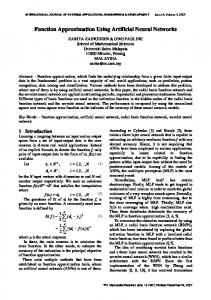
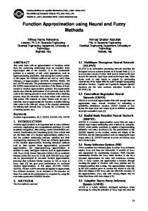
are chosen as transfer function. The two curves (the task and its best approximation), after a transient close comparison, deviate from each other. This deviation becomes less pronounced when using Gaussian functions [f(x) =A exp (-((x²)/2))] as can be seen on figure 2. This fact is principally due to the Gaussian shape which seems to be more appropriate than sigmoid to approximate the target task (Eq.7). Next, we expand Fapp in terms of, first, a "Morlet" wavelet family [f(x )= cos (6x) exp(-((x²)/2))] and, second, a " Mexican hat" one [f(x)=(1-x²)exp(((x²)/2))] and the results are displayed in figures 3 and 4, respectively. Interestingly, we note a net improvement when compared with the two former cases (in particular, in the case of the "Mexican hat" family). Consequently, it makes clear that the choice of the basic functions strongly influences the quality of the approximation. Next, to show the performance of the network used, consider the function F(x) = x Sin(x), defined in the interval [0,10].We choose N=5. After 71steps, the results of the function and its best approximation are depicted in figure 5. We have then considered two other tasks : F(x)=exp(-5x)sin(2πx), defined in the interval [0,1] and F(x) = exp(-(x+1)/2) x sin(3x+7), defined in the interval[0,2]. As illustrated in figures 6 and 7 respectively, the tasks and their best approximations are close to each others. We have then considered three simpler and smooth tasks (F(x) = cos (x), F(x) =sin(x), F(x) = tanh (x)). Obviously, it is apparent that the chosen network approximate very well these functions as can be seen on figures 8,9 and 10 respectively.
-446-
F 0.4 0.3 0.2 0.1 X 5
10
15
20
-0.1
Figure 1. Plot of the task (solid line) and its best approximation (dashed line) in the case of the sigmoid.
F 0.4 0.3 0.2 0.1 X 5
10
15
20
-0.1
Figure 2. Plot of the task (solid line) and its best approximation (dashed line) in the case of Gaussian.
F 0.4 0.3 0.2 0.1 X 5
10
15
20
-0.1
Figure 3. Plot of the task (solid line) and its best approximation (dashed line) in the case of the Morlet wavelet.
-447-
F 0.4 0.3 0.2 0.1 X 5
10
15
20
-0.1
Figure 4. Plot of the task (solid line) and its best approximation (dashed line) in the case of the Mexican hat wavelet. 0.6 0.4 0.2
2
4
6
8
10
-0.2 -0.4 -0.6
Figure 5. Plot of the task (F(x) = x sin(x), solid line) and its best approximation (dashed line) 2 1.5 1 0.5
0.2
0.4
0.6
0.8
1
Figure 6. Plot of the task (F(x) = exp(-5x) sin(2pix), solid line) and its best approximation (dashed line).
-448-
0.5
0.5
1
1.5
2
-0.5
-1
Figure 7. Plot of the task (F(x ) = exp(-(x+1)/2)x sin (3x+7), solid line) and its best approximation (dashed line).
0.75 0.5 0.25 0.5
1
1.5
2
2.5
3
-0.25 -0.5 -0.75
Figure 8. Plot of the task (F(x) = cos (x), solid line) and its best approximation (dashed line).
0.8
0.6
0.4
0.2
0.5
1
1.5
2
2.5
3
Figure 9. Plot of the task (F(x) = sin(x), solid line) and its best approximation (dashed line).
-449-
0.7 0.6 0.5 0.4 0.3 0.2 0.1 0.5
1
1.5
2
2.5
3
Figure 10. Plot of the task (F(x) = tanh (x), solid line) and its best approximation (dashed line). It is worth to note that the number of formal neurons to be used for training cannot be computed in advance: too few numbers lead to inadequate knowledge about the function, while too many pairs make training slow. Furthermore, we found that only a few number of units are needed for "smooth" functions whereas more units are required for wildly fluctuating functions.
VI- CONCLUSION To summarize, we have investigated as many properties as possible of neural nets made of "artificial neurons" used for function approximation. Attention has been devoted to the role transfer functions may play during and after the learning process. Firstly, we have investigated the universal approximation theory of neural networks whose transfer functions are: sigmoids, Gaussian and two specified families of wavelets. The latter have been found to be more appropriate to use. It is worth to note that none of the functions mentioned above is flexible enough to describe an arbitrarily shaped function and be optimal in all cases. It depends widely on the form of the function to approximate. Then, by considering different tasks relevant and inherent to various applications in physics, we showed that a simplified architecture provides a reasonably efficient, practical and robust, multifrequency analysis. In fact, a reconstruction of tasks has occurred very well with a relatively small number of units and iterations for all our numerical implementation carried out over a wide range of task functions. REFERENCES [1] Hopfield, J.J. and Tank, D.W., Sciences 233, 625 (1986). [2] Haykin, S., Neural Networks, New York: Macmillan, 1994. [3] Hornik, K., Stinchcombe, M., and White, H., Neural Networks 2, 359 (1989). [4] Giraud, B.G. and Touzeau, A., Phys. Rev. E 65, 01609 (2001). [5] Mallat, S., IEEE Trans. Pattern Anal. Machine 11, 674 (1989). [6] Cybenko, G., Mathematics of Control, Signals and Systems 2, 303 (1988). [7] Hartman, E.J., Keeler, J.D., and Kowalski, J.M., Neural Computation 2, 210 (1990). [8] Arik, S., Chaos, Solitons & Fractals 26, 1407 (2005). [9] Liang, J., and Cao, J., Chaos, Solitons & Fractals 22, 773 (2004).
-450-