Nucl. Instr. and Meth. A, in press DFUB 94/16
Results from an On-Line Non-Leptonic Neural Trigger Implemented in an Experiment Looking for Beauty C. BALDANZA, F. BISI, A. COTTA-RAMUSINO, I. D'ANTONE, L. MALFERRARI, P. MAZZANTI, F. ODORICI, R. ODORICO*, M. ZUFFA INFN ANNETTHE, Via Irnerio 46, 40126 Bologna, Italy C. BRUSCHINI, P. MUSICO, P. NOVELLI INFN/Genoa, Via Dodecaneso 33, 16146 Genoa, Italy M. Passaseo CERN, 1211 Geneva 23, Switzerland
ABSTRACT Results from a non-leptonic neural-network trigger hosted by experiment WA92, looking for beauty particle production from 350 GeV negative pions on a fixed Cu target, are presented. The neural trigger has been used to send events selected by means of a non-leptonic signature based on microvertex detector information to a special data stream, meant for early analysis. The non-leptonic signature, defined in a neural-network fashion, was devised so as to enrich the selected sample in the number of events containing C3 secondary vertices (i.e, vertices having three tracks with sum of electric charges equal to +1 or -1), which are sought for further analysis to identify charm and beauty non-leptonic decays. The neural trigger module consists of a VME crate hosting two MA16 digital neural chips from Siemens and two ETANN analog neural chips from Intel. During the experimental run, only the ETANN chips were operational. The neural trigger operated for two continuous weeks during the WA92 1993 run. For an acceptance of 15% for C3 events, the neural trigger yields a C3 enrichment factor of 6.67.1 (depending on the event sample considered), which multiplied by that already provided by the standard trigger leads to a global C3 enrichment factor of ~150. In the event sample selected by the neural trigger, one every ~7 events contains a C3 vertex. The response time of the neural trigger module is 5.8 µs.
*
E-mail:
[email protected], 38239::odorico
2
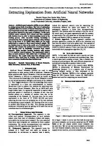
1. Introduction The idea of developing signatures for the dominant non-leptonic decays of heavy flavor particles by exploiting statistical correlations within the associated events was put forward some time ago [1,2]. The technique proposed at that time was Fisher's linear discrimination [3], which corresponds to a simple Feed-Forward neural network with one input and one output layer and a single output neuron. The recent appearance of neural microprocessors, able to implement multi-layered neural networks with response times of a few microseconds, has stimulated efforts for the realization of on-line neural triggers capable of exploiting non-leptonic signatures of heavy flavors in high luminosity particle accelerators. Projects of this type were announced at the IEEE 1992 Nuclear Science Symposium [4-6]. So far, the only hardware development presented consists of a commercially available VME card, ELTEC SAC-711 [7], hosting the ETANN chip [8] which has been used off-line with simulated events [9]. The neural trigger module, whose realization and on-line running results are presented here #, consists of a VME crate utilizing the neural chips ETANN (analog) from Intel [8] and MA16 (digital) from Siemens [11] which has operated within the WA92 experiment at CERN [12] during the 1993 run. WA92 is an experiment looking for the production of beauty particles by a π− beam at 350 GeV/c impinging on a Cu target. Task of the Neural Trigger was to select events by exploiting a non-leptonic decay signature and to accept them into a special data stream, meant for early analysis. Specifically, the Neural Trigger was trained to enrich the fraction of events with C3 secondary vertices, i.e. branching into three tracks with sum of the electric charges equal to +1 or -1. C3 vertices are sought for further analysis aimed to identify charm and beauty non-leptonic decays. The off-line reconstruction of C3 vertices makes largely use of data from the fine-grained silicon microstrip Decay Detector [13], which has a slow response and cannot be used for triggering. In order to enrich the fraction of C3 events in the selected sample, the Neural Trigger exploits statistical correlations characteristic for C3 events among quantities which can be calculated on-line from the hits measured in the silicon microstrip Vertex Detector, which has a fast response and can be used for triggering. Such correlations are "learned" by the neural network, loaded on the Neural Trigger, in a previous off-line stage (the training stage). During training the neural network is presented with two separate event samples, which have been certified off-line as containing and not containing, respectively, C3 vertices. An
# A preliminary presentation has been made in [10].
3
appropriate training algorithm changes the internal parameters of the neural network so that its response becomes as widely different as possible for the two classes of events. The training of the neural network was done using WA92 data collected in the 1993 run, with C3 events certified off-line by the Trident event reconstruction program. The events used had been accepted by the WA92 standard trigger, so that the task of the Neural Trigger was to provide additional C3 enrichment for the events it accepted into the special data stream. Input to the Neural Trigger was provided by the Beauty Contiguity Processor (BCP) [14,15], which determined tracks and their impact parameters on-line, using hit locations in the silicon microstrip Vertex Detector. The BCP output, arranged in five 64-bit hit-maps each one corresponding to separate impact parameter windows, was preprocessed within the neural crate to yield 16 input variables for the neural chips. At the time of running only the ETANN part of the crate was operational, with the MA16 part still waiting for completion of the debugging of the MA16 microcode. The Neural Trigger has been in operation for two weeks, during which its stability was verified. Section 2 introduces the basic concepts entering neural network applications to high-energy physics triggers. Section 3 describes the parts of the WA92 trigger apparatus relevant for the Neural Trigger. Section 4 presents the main characteristics of the Neural Trigger hardware. Section 5 specifies the neural network architecture and the training procedure employed in the present trigger application. Section 6 presents and discusses the results of the Neural Trigger for the 1993 WA92 run. Section 7 reports on the stability checks made on the Neural Trigger. Section 8 contains the conclusions.
2. Neural Networks An introduction to artificial neural networks suited for applications in highenergy physics can be found in [16]. Here, only the basic concepts are presented. Suppose we wish to discriminate from each other two classes of events, A and B, on which two event variables, s1 and s2, are measured (they can represent event shape variables or whatever else), and suppose that the class distributions in the two event variables are those of Fig. 1. If we try to discriminate class A events from class B events by a conventional cut on the single-variable distribution obtained by projecting the entries over the s1 axis, we will either lose a large fraction of A events when trying to get a pure A sample or tolerate a large contamination when trying to keep a high acceptance for A events. The same occurs when projecting over the s2 axis. But if we project over the axis labeled as Fisher axis [3, 17], the two resulting class distributions
4
do not overlap and, by imposing a cut in the middle, one gets a clean separation without any loss of acceptance for A events. The essential ingredient one is exploiting is that both in A and B events the two variables s1 and s2 are correlated and that the correlation is different within the two event classes. The projection over the Fisher axis, i.e. the Fisher discriminant variable, can be written as a = ∑k ωk sk + θ The Fisher discriminant represents the simplest type of Feed-Forward neural network, having 1 layer and 1 output neuron, a representing the activation of the neuron. Its internal parameters, the weights ω k and the threshold θ , can be straightforwardly determined from the centroids and the correlation (or covariance) matrices of the two event classes. One can easily show that if the two class distributions are gaussian shaped and have the same correlation matrices, no other discriminant can outperform the Fisher discriminant. If the distributions are far from gaussian and, in particular, they exhibit concavities (think e.g. of a banana-shaped distribution) the simple Fisher discriminant may turn out to be inadequate. In Fig. 2 the extreme case is represented of a uniform B distribution shaped like a ring, containing the A distribution in its interior. It is clear that there is no single axis over which the two distributions get separated. A way out is provided by iterating the Fisher construct. Namely, by introducing more axes defining new coordinates (1st layer), and using them again as input to a Fisher discriminant (2nd layer). If the coordinates obtained from the 1st layer were directly used as input to the 2nd layer, however, the activation of the 2nd layer neuron would depend linearly on s1 and s 2 , and thus we would fall back to a single Fisher discriminant, without any improvement. That is changed if before passing the activations of the 1st layer neurons (also called hidden neurons) to the input of the 2nd layer neuron we first filter them through a non-linear transfer function g(a), which is generally chosen as a saturating monotonic function like the hyperbolic tangent: x = g(a)= tanh(a) It is convenient to apply g(a) also to the activation of the 2nd layer neuron, yielding the output of the net, so as to have a well defined output domain. Of course, one may also consider neural nets with more than two layers, by simply iterating the structure, and one may have several output neurons (e.g. when there are more than two classes to discriminate amongst). The determination of the internal parameters must now proceed
5
through a sometimes lengthy iteration process, called training. One must fix output targets for each class, and for each input event consider the distance of the corresponding output from its class target and then find (e.g. using the BackPropagation algorithm [18]) its derivative with respect to each single internal parameter and change its value accordingly, so as to reduce the distance (i.e. by a conventional steepest-descent method). The set of events is presented over and over until no sensible improvements are made in reducing discrepancies. The discrimination problem of Fig. 2 can be solved by a Feed-Forward net, see Fig. 3, with one hidden layer consisting of 3 neurons, defined by the 3 axes a1, a2 and a3 shown in Fig. 2 (the distance along the axes is 4.5 times the euclidean distance in the metric of the variables), and with equal weights for the output neuron. That comes from training with the Back-Propagation algorithm, which in this (relatively rare) case also rejects a fourth hidden neuron (i.e. it is left with vanishing weights). In general, the optimal architecture of the net, i.e. the numbers of neurons for each layer, has to be found by trial and error. The example of Fig. 2 also shows the relevance of the non-linear transfer function. It is well known that the sum of the coordinates of any point along three such axes is independent of the point, and thus with a linear g(a) the net would give a constant value independent of the event. Feed-Forward nets, although more versatile than the Fisher discriminant, may be inadequate for some discrimination tasks. E.g., for the problem of Fig. 4 no solution has been found with a standard net, like those described above [19]. Of more general applicability are neural networks of the Learning Vector Quantization (LVQ) type [20]. In these nets neurons correspond to points in the variable space, and they are labeled by one of the classes considered: in the example of Fig. 2 there are neurons of class A and neurons of class B. During training, each event corrects the position of the neuron closest to it: it moves the neuron closer to itself if it belongs to its same class, otherwise it moves it farther away from itself. The event set is repeatedly presented until no sensible changes are made. During classification, an event is classified into the class of neuron closest to itself. In Fig. 2, white and black points represent such neurons, as they result from training. In practical applications, where distributions overlap to some extent, this simple scheme does not allow to estimate how safe the classification is, differently from Feed-Forward nets where one can use the distance of the output from the class target. That can be done by attaching to each neuron a counter for each class, counting how many times the neuron has been trained by events of that class (LVQTC: Learning Vector Quantization with Training Counters [21]). The fraction of times the neuron has been trained by events of its same class gauges how much reliable the classification provided by the neuron is. Going back to the example of Fig. 4, it is clear that it can be easily solved by LVQTC. In comparison with Feed-Forward nets, LVQTC
6
typically requires more internal parameters, since one has to cover distributions by sets of points in contrast to Feed-Forward nets where distributions get separated by hyperplanes, whose normal vectors define coordinate axes. From the examples discussed, it is apparent that the choice of the discriminant largely depends on the problem at hand. One should also keep in mind that a change in the variables used may completely modify the nature of the discrimination problem. For instance, if in the example of Fig. 2 one uses the squares of s1 and s2 as variables, the problem can be exactly solved by a Fisher discriminant, amounting to the variable (s1)2 + (s2)2. When picking up a discriminant and choosing its architecture one must care to keep the number of internal parameters as small as possible in order to cope with the generalization problem: with too many internal parameters the discriminant can become the quasi-equivalent of a look-up-table, giving a good performance on the training set but behaving badly on new test events because of the intervening statistical fluctuations. In on-line trigger applications in high-energy physics, a related concern is robustness: the class distributions may change their shapes with time, because of temperature excursions (affecting alignments, level of electronic noise etc.) and possible degradation of parts of the experimental apparatus. That often translates into another reason for keeping the number of internal parameters low, so as to avoid counterproductive fine adjustments to volatile details of the class distributions. When implementing the neural network on a dedicated chip, the number of internal parameters must be anyway comply with the hardware limitations. Since for a given problem a Feed-Forward net often entails a smaller number of parameters than a LVQTC net, most of the neural chips available are meant for nets of the Feed-Forward type (the MA16 chip, though, accommodates both types of nets). With a neural chip implementation, one must also care about the limited precision offered by the hardware when developing the neural net. In a Feed-Forward net the calculation of a neuron activation may involve delicate cancellations and the associated effects pile up as one moves up to subsequent layers. Therefore, if precision represents a relevant issue it is advisable to keep the number of layers to a minimum. That is especially true for an analog chip like ETANN, whose precision is of the order of a few percents [8, 22]. It is less relevant for the digital MA16 chip, which has a 16-bit precision for input and output, and an intermediate precision of 48 bits [11]. Also hardware limitations on the number of input variables and the speed with which they are loaded on the chip must be taken into account when developing the neural network. ETANN can accept up to 128 input variables with a 1-layer net, which reduce to 64 with a 2-layer net (because of the limited weight storage). If one can directly use analog input
7
signals, they can all be loaded in parallel on the chip. MA16 loads the input variables sequentially with no a priori limitations on their number, but of course the more they are the higher becomes the number of clock cycles necessary to get the chip response.
3. Input from the WA92 Apparatus The part of the WA92 trigger detector [12] relevant for the input to the neural chips (see Fig. 5) consists of 6 silicon microstrip planes of the Vertex Detector (VD), measuring the z coordinates of tracks, where the z axis has the direction of the magnetic field (bottom-up direction). The last plane is positioned at about 41 cm downstream of the target and has a square shape with a 5 cm side, centered around the beam. The hit information from the 6 planes is processed by the Beauty Contiguity Processor (BCP) [14], which reconstructs tracks and their impact parameters (IP), with a global response time of about 40 µs [15]. IP is defined as the signed difference between the z value of the track extrapolated back to the target-center plane and the beam z position. The BCP supplies to the Neural Trigger 5 words of 64-bit each, plus a standard go-ahead termination word. Each one of the 5 words directly represents the hit-map of tracks on the last (6th) VD layer, divided in 64 bins, for tracks falling within a given IP window. The 5 IP windows used are, in µm: -200 < IP < 200, 200 < IP < 400, -400 < IP < -200, 400 < IP < 900, -900 < IP < -400. The BCP could supply up to 8 hit-maps, with a resolution which can reach 256 bits. Data transfer times would be correspondingly increased. Simulation has shown that the arrangement we eventually employed is adequate for the task and does not lead to any significant loss of performance. The BCP also makes a first level decision about accepting the event. Defining as secondary tracks those with |IP| > 100 µm and as primary the other tracks, the BCP Trigger (BCPT) requires the presence of 3 primary tracks, 2 secondary tracks and 1 track in the Butterfly Hodoscope with high pT (defined in a detector dependent mode, roughly corresponding to > 0.6 GeV/c along the z axis). The Neural Trigger considers only events which have already been accepted by the BCPT. Off-line reconstruction of the primary and secondary vertices in the events makes largely use of the fine-grained Decay Detector, which consists of a set of densely packed microstrip planes located right behind the target [13]. Its response time is too long to make it usable for triggering.
4. Neural Trigger Hardware
8
A detailed presentation of the Neural Trigger hardware will be made elsewhere [23]. Here we only report its main features. The Neural Trigger consists of an extended VME crate, which is schematically shown in Fig. 6. A VIC board from CES interfaces the VME bus to a Personal Computer for control and monitoring operations. It also allows to simulate on-line running conditions for testing, having recorded experimental inputs or simulated inputs passed through the crate with subsequent collection of the corresponding outputs. The Interface Board receives the five 64-bit words plus a termination word from the BCP. It also receives control bits, in particular the burst and strobe bits for synchronization with the beam pulse. It was designed to also receive input from the Butterfly Hodoscope, signaling the presence of high pT particles, but eventually these data were not used. The 4 Preprocessing Boards host 2 independent Preprocessing Unit each. A Preprocessing Unit calculates the input variables referring to a given IP window which enter the neural chips. With 5 IP windows, only 5 such units are actually used. The ETANN board hosts two independent ETANN chips. The Intel's 80170NX Electrically Trainable Analog Neural Network device is an analog chip which is commercially available together with a development system, the iNNTS [22]. Neural weights are stored in the chip in EEPROM-like fashion. iNNTS includes a hardware box (the trainer) where to insert the chip, which is interfaced to an IBM-compatible personal computer, and software to be run on the PC so as to allow read and write operations for the neural weights and processing of the input patterns through the chip. The chip can operate in 1-layer mode, accepting a maximum of 128 input variables, and in 2-layer mode with a clocked-back feedback operation, accepting a maximum of 64 input variables. In both cases, it has 64 independent outputs (thus, a maximum of 64 hidden layer nodes in the 2-layer mode). We have measured response times of 1.5 µs for the 1-layer mode and of 4.5 µs for the 2-layer mode. We have then chosen to allow safer processing times of 2.6 µs for the 1-layer mode and of 6.1 µs for the 2-layer mode. Adding to the response time from the chips the time spent in the Interface and Preprocessing Boards and data transfer, which is 3.2 µs, one has a total response time for the Neural Trigger module of 5.8 µs for the single-layer net we have actually used. That would grow to 9.3 µs for a 2-layer net. Precision of the chip is quoted [8] as being equivalent to 6-7 bits. Operatively, with our set-up, after conversion of the output to a 8bit digital number (range 0-255), we have found during the experimental run a
9
maximum deviation of 4 units for a high response (i.e., around or above the trigger threshold value) and a maximum deviation of 6 units for a low response, when routinely sending a prefixed set of test patterns in input to the chip. A critical feature of ETANN is its dependence on the values of the power supply voltage (about 5 V) and on its temperature. In particular, one must care that these values remain stable when moving the chip from the iNNTS trainer to the board. In order to eliminate these problems, we have developed an ETANN Controlled Environment (ECE) Unit consisting of a daughter board detachable from the main board and fit to be inserted in the iNNTS trainer. In the ECE Unit, ETANN is serviced by a voltage regulator, stabilizing its power voltage to within ∆V ≤ 5 mV, and a temperature controller stabilizing its temperature at 18 ˚C to within ∆T ≤ 1 ˚C. The temperature controller is based on Peltier's cells from MELCOR, and absorbs up to 15 W versus the 5 W dissipation of ETANN. Because of its high power consumption, the temperature controller has a separate power supply. Prominent analog operating parameters can be monitored via VME. Input variables from the Preprocessing Boards are converted to analog signals for ETANN by 8-bit Digital to Analog Converters (DAC's). The range of the input variables is 0-16, therefore 8-bit precision is sufficient. 32 variables can be accepted in input by the board, but we used only 16 of them. The 8-bit input is converted to an analog signal from 1.6 to 3.2 V, with zero corresponding to V REFI = 1.6 V, as required by ETANN. The output from ETANN, ranging from 0 to 3.2 V, is converted by Analog to Digital Converters (ADC's) to an 8-bit digital number in the range 0 to 255. The converted output is compared with a preset threshold value for triggering in a comparator, which leads to the generation of the corresponding trigger bit as a NIM signal. The parameter controlling the transfer function slope has been set at V GAIN = 4.0 V. In the iNNTS trainer, we have set the zero reference value for the output at V REFO = 1.6 V. (For detailed specifications of the ETANN control parameters see [8].) For comparison, we also give the main characteristics of the MA16 boards, which did not operate during the 1993 WA92 run. The MA16 is a digital microprocessor of systolic type supplied by Siemens as a prototype [11]. It has 16-bit precision for the input and output and has an internal precision of 48 bits. It requires external storage for the neural weights, the transfer function and the controller. The MA16 board has been designed to accommodate 16 input variables, a 2-layer FeedForward neural net with a maximum of 15 hidden nodes and a Fisher discriminant. The response time of the board at 50 MHz is 5.2 µs. Adding to it the time spent in the
10
Interface and Preprocessing Boards, which is 3.2 µs, one has a total response time for the MA16 part of the Neural Trigger module of 8.4 µs.
5. Neural Network Architecture and Training In principle, we could have set as target for the Neural Trigger the direct recognition of beauty particle decays, defined by simulated events obtained by an event generator with added GEANT simulation of the WA92 apparatus. However, we refrained from doing that mainly for two reasons: i) although such simulated events were available, they were suitable for off-line studies, but were not appropriate for quantitative tuning of a neural trigger, because of the general dependence of event generators on model assumptions which are especially critical for the correlations involving the relatively low mass beauty particles and a complex nuclear target like copper; ii) the necessity of depending on graphical scanning, with the long waiting times involved, to have indications on the actual performance of the Neural Trigger. Taking into account the effective necessities of the experiment, which required the analysis of many tens of millions of events to extract the few thousands affordable by graphic scanning, we rather focused on the enrichment in events which are selected for that sake. Especially interesting, from this point of view, are events with C3 secondary vertices, branching into three tracks with sum of electric charges equal to ± 1. A C3 vertex may be due to a D → Kππ decay, which in its turn may be originated by the decay of a beauty particle. Certification of these events comes from the Trident event reconstruction program. By applying the event reconstruction program to real data obtained with a given experimental set-up, one gets the necessary event training samples to tune the Neural Trigger for enrichment in C3 events with the same experimental setup. In this way one avoids altogether dependence on theoretical modeling and only relies on the event reconstruction program. This is the target we have chosen for the Neural Trigger. In doing that the Neural Trigger does not act alone, but in conjunction with the BCP Trigger (BCPT, see Section 3): only events already accepted by the BCPT are worked out by the Neural Trigger. By concentrating on BCPT events only, the Neural Trigger can better focus on statistical correlations present within the events which discriminate signal from background. An example of them is offered by angle-IP correlations for tracks. As shown in Fig. 7 the angular distribution of tracks is strongly correlated to the sign of IP for C3 events, while this correlation is marginal for background events. The non-leptonic signature represented by the combination of the BCPT and the Neural Trigger has been used to send events to a special data stream, meant for early analysis.
11
In order to train the neural net, one not only needs to have samples of signal and background events certified by the event reconstruction program, but also to have the corresponding input patterns to the neural chips calculated from them. As specified in Section 3, input variables to the neural chips are calculated from the BCP output, but the latter is not recorded on the event tapes. To recover it we used the BCP simulator, which exactly reproduces the BCP calculations [24], applied to the raw data on tape. In order to design the neural net architecture and to chose the input variables, we could not wait for the 1993 data being made available, but we had to rely on the 1992 WA92 data obtained with a somewhat different BCPT set-up. Since the 1993 BCPT included in part the angle-IP correlations exploited in the preliminary neural net studies on the 1992 data, it turned out that some of the input variables which had been chosen had become irrelevant. Performance of the Neural Trigger has degraded to some degree because of that. Only input variables simple to calculate with the available hardware were taken into consideration. The basic strategy in devising them was to have them convey multi-scale information on the hit maps provided by the BCP. We first considered the maximum resolution made available by the BCP: 256 bits. By directly studying the corresponding hit maps for a set of events, however, we saw that 64-bit hit maps were enough. Using such a resolution had the advantage of reducing transfer times and simplified the collection of the hit maps from the BCP by employing an already existing but unused 64-bit output connector. We then considered variables counting the number of hits with 1-bit, 4-bit, 8-bit, 16-bit, and 32-bit resolutions. We submitted them to significance tests based on Fisher discrimination [16, 17]. It turned out that the significant variables were those associated with 1-bit and 16-bit resolutions. The study was made by varying the IP window segmentation. Eventually, we found that an adequate IP window segmentation was the following one (the BCP allows for a maximum of 8 IP windows): #IP 1 2 3 4 5
Range (µm) -200 200 -400 400 -900
< IP < 200 < IP < 400 < IP < -200 < IP < 900 < IP < -400
As to the choice of variables, we found that the following 16 variables were adequate according to significance tests based on Fisher discrimination. Each 64-bit map (#IP = 1-5) is divided in 4x16-bit groups, ordered bottom-up in z, and on the basis of that the following variables are defined:
12
K16MAP(i) K16 KDW16 KUP16
= #hits in group i = 1-4 = #groups hit = #groups in bottom half hit = #groups in top half hit
(range: 0-16) (range: 0-4) (range: 0-2) (range: 0-2)
The 16 variables which have been chosen are: #
VARIABLE
#IP
1 2 3 4 5 6 7 8 9 10 11 12 13 14 15 16
K16 K16MAP(1) K16MAP(4) KDW16 K16MAP(1) KUP16 K16MAP(3) K16MAP(4) KDW16 K16MAP(1) K16MAP(2) K16MAP(3) KUP16 K16MAP(2) K16MAP(3) K16MAP(4)
1 1 1 2 2 3 3 3 4 4 4 4 5 5 5 5
The slight asymmetry between windows with opposite IP is a reflection of the similar asymmetry observable in angle-IP correlations, Fig. 7. That is due to the fact that the BCP seeks the beam particle searching from bottom up and that there is a substantial fraction of events with two beam particles, one of which is just passing through. If the latter is picked up by the BCP as the actual beam particle in the event, one gets a spurious determination of the IP of tracks leading on average to the above asymmetry. One can argue against reliance on significance tests based on Fisher discrimination for choosing the input variables, regarding them as appropriate when discussing the separation of the bulk of the event class distributions but too insensitive to the tail structure of these distributions, which is in principle relevant in high enrichment applications. Being aware of that, in our preliminary neural net studies we
13
made several tries with larger samples of input variables, taken from the large original pool. But we got no significant improvement of the results. For the neural net architecture we considered the two options offered by ETANN: a 2-layer or a 1-layer net, the latter being equivalent to a Fisher discriminant. As discussed in Section 2, the optimal type of neural net totally depends on the problem at hand. If the two class distributions one has to discriminate from each other have gaussian shapes with similar correlation matrices, no classifier can outperform the Fisher discriminant. We made preliminary software studies simulating some of the ETANN restrictions, as represented by the software handling the iNNTS development system. Specifically, weights and thresholds were requested to stay between -2.5 and 2.5 with input variables limited to stay within -1 and +1. No useful way was found to simulate the limited weight precision. After training by standard back-propagation, the 2-layer net gave results slightly better (of the order of 20%) than a 1-layer net. But, after loading the nets on ETANN and having made some chip-in-loop training of the 2-layer net (that is not necessary for a 1-layer net), we found that the small margin in favor of the 2-layer net evaporated. Looking in detail at how event patterns were processed in the 2-layer net, we realized that the net had organized itself so that discrimination between the two event classes was largely due to small differences between the responses of the first layer which entered cancellations performed by the second layer node. Thus, weight precision had a large incidence on the results. We found no way of forcing backpropagation to direct the organization of the net to a structure less sensitive to weight precision. (Procedures to compensate for the limited weight precision by separately changing the transfer function slopes of nodes [19] are not applicable to ETANN, which has a single parameter, VGAIN, to control all the, nominally, equal slopes.) We had other reasons pressing us toward a 1-layer architecture: i) simplicity of training, since a 1layer net, i.e. a Fisher discriminant, requires only inversion of the pooled-over-classes correlation matrix for that sake; ii) avoidance of chip-in-loop training, which may burn out nodes in ETANN, since it is mainly required by the hardware differences of the transfer functions between nodes, which become irrelevant for a 1-layer net with one output node; iii) increased robustness towards changes in the operating conditions of the trigger detector, e.g. due to temperature excursions which can change alignments and the level of electronic noise, since the net is less fine-tuned to details of the shapes of the event class distributions; iv) shortening of the response time of the Neural Trigger. In conclusion, we adopted a 1-layer net architecture with one output node. Its weights (i.e. the Fisher vector components) were determined on a conventional workstation by a simple matrix inversion operation and then loaded on ETANN by means of iNNTS. The procedure was fast and straightforward, in compliance with the
14
strict time restrictions we had to meet during the experimental run. The training event samples we used consisted of 3,000 C3 events and 10,000 non-C3 events, accepted by the BCPT. The collection of the C3 event sample required the running of the Trident event reconstruction program for about 4 days on 3 alphavaxes 3000/400. C3 vertices are defined by the Trident event reconstruction program, release 11, requiring in addition: i) IP in the y-z plane (orthogonal to the beam direction) > 60 µm, ii) distance in x from the primary vertex > 6 σ, iii) x of the vertex not before the target and not beyond the Vertex Detector, iv) at least two tracks with |IP| along the z direction > 20 µm.
6. Results from the Experimental Run The Neural Trigger, after its training was completed, operated for two continuous weeks within the apparatus of WA92. The results we present are based on samples of events collected in September 1993, while the training sample dates back to mid August, and they where chosen a few days apart to check for stability. The neural net loaded was organized so as to have an high response from ETANN for C3 events. After conversion to a 8-bit digital number, the response from the two ETANN chips comes in the form of an integer number ranging from 0 to 255. The trigger bit was activated when the response from the ETANN chosen for triggering (the other one was used for cross checks) was above a preset threshold, chosen on the basis of a tradeoff between acceptance and enrichment for C3 events and also taking into account other considerations, like the trigger rate. Specifications of the event samples used for testing are given in Table 1. Figs. 8 and 9 show the dependences on the trigger threshold of the acceptance and the enrichment for C3 events given by the Neural Trigger, applied to events already selected by the BCP Trigger. The figures refer to the two ETANN chips, labeled ETANN_0 and ETANN_1, respectively. Moving up the trigger threshold, the C3 enrichment factor increases up to a value of ~7. To better see the tradeoff between enrichment and acceptance, one can remove the horizontal axis and plot C3 enrichment directly versus the corresponding C3 acceptance, as done in Figs. 10 and 11. First of all, from comparing the two last figures one can verify that the two chips give perfectly consistent results. Also the curves of Figs. 8 and 9 superimpose if when moving from ETANN_0 to ETANN_1 the threshold value is increased by about 5 units. That is not surprising since being ETANN an analog chip, two chips do not share identical characteristics. In particular, the transfer function applied to the output node is likely to have different offset and slope values in the two chips. On the other hand, that is not
15
relevant since the trigger threshold is set for each chip by looking at the enrichment and acceptance it actually gives on the chip, as gauged on a test sample independent of the training sample. The small deviations in performance, observable when moving from one event sample to another, do not appear to be due to the Neural Trigger itself, which has been verified to be stable by independent tests discussed in the next section, but are likely due to slight modifications in the experimental apparatus, e.g. caused by temperature excursions. The overall stability of the Neural Trigger performance rather shows its robustness toward changes in the external conditions. From Figs. 10 and 11 one can read that for a C3 acceptance of 15% one obtains a C3 enrichment factor of 6.6-7.1, depending on the event sample. That is just the factor by which the C3 enrichment already given by the BCPT is boosted up. The global C3 enrichment factor provided by the BCPT and Neural Trigger combination is found to be ~150, with a statistical error of ~30%, due to the limited statistics available for interaction trigger runs (i.e. with the BCPT turned off). The corresponding global C3 acceptance is ~1%. Its smallness is largely due to the fact that in the off-line event reconstruction C3 vertices are requested to have two tracks with |IP| > 20 µm (using the data from the high-resolution microvertex Decay Detector, not usable for triggering), whereas the BCPT (using only data from the low-resolution Vertex Detector) requires two tracks with IP| > 100 µm. In the sample of events accepted into the special data stream by the BCPT times Neural Trigger combination, 1 every ~7 events is found to have a C3 vertex (reconstructed by Trident release 12).
7. Stability Since ETANN is an analog chip, routine checks have been made during on-line operations on its proper performance. The power supply voltage and the temperature of the two chips have been constantly monitored, with alarms set if their values moved outside allowed tolerances. A set of 20 prefixed input patterns were sent in input to the Interface Board of the Neural Crate via the VME bus during out-of-burst periods. The patterns were selected so that the corresponding responses from the chips were distributed uniformly in the interval of interest around the trigger threshold (i.e. in the range 90-180). When presented with the same input pattern repeatedly, an ETANN chip never gives exactly the same response, its (analog) precision being of the order of a few percents. Table 2 lists, for each chip, the deviations of the responses observed over a number of days during the run with respect to the corresponding values given at the
16
beginning of the run, picking up each day one of such tests at random. The statistical entries of the Table refer to one set of 20 patterns. No evolution with time of the deviations, however gauged, is observed. The mean value, including sign, of the deviation and its root mean square variance are never larger than 2 units (the output range is 0-255). The maximum deviation reaches up to 6 units for ETANN_0 and 4 units for ETANN_1. But, for patterns whose (original) output values lie in the range of interest for the trigger threshold setting (i.e., > 130 for ETANN_0 and > 134 for ETANN_1), the maximum deviation reaches up to 4 units for ETANN_0 and 3 units for ETANN_1. That is due to the fact that low output values are attained through stronger cancellations in the linear combination determining the output, which is then made more sensitive to the limited precision of ETANN. A qualitative on-line check of the Neural Trigger is provided by the stability of the trigger rate. Fig. 12 shows the distribution of runs (each run yielding on average about 24,000 events) in the mean number of triggers per pulse of the Neural Trigger and the BCPT. In the presence of a relative stable BCPT rate also the Neural Trigger rate appears stable. Fig. 13 illustrates more directly the time evolutions of the two trigger rates (trigger rates are truncated to integer values by the monitoring software of the experiment). Off-line checks of the stability of the combination of the BCPT with the Neural Trigger are obtained by comparing enrichment results for event samples collected over separate periods of time and by cross-checking results from the two ETANN chips. Such comparisons have been presented in the previous section.
8. Conclusions A Neural Network Trigger device based on the ETANN chip has been demonstrated by two weeks of continuous running in the experiment WA92, looking for the production of beauty particles. Task of the Neural Trigger was to select events containing C3 secondary vertices (i.e. with three tracks, having sum of electric charges equal to ±1) and to accept them into a special data stream, meant for early analysis. This is the first demonstration of a Neural Network Trigger implemented on-line in an highenergy physics experiment. The device has been shown to be stable during the running period and robust enough to yield a performance essentially independent of the detailed characteristics of the experimental trigger apparatus, subject to changes because of temperature excursions and other reasons. Used in combination with the standard BCP Trigger of the experiment, which exploits in a simpler way data from the microstrip
17
Vertex Detector reconstructed into tracks by the Beauty Contiguity Processor, the Neural Trigger yields an enrichment by a factor ~150 for the fraction of events containing C3 secondary vertices. The event sample which is eventually selected contains one event with a C3 vertex about every ~7 events, when setting the C3 acceptance of the Neural Trigger relative to the BCPT at 15%. The response time of the Neural Trigger module is 5.8 µs. It is understood that the above results are for enrichment in C3 events which, besides including heavy-quark events, also contain a substantial background. Tuning the neural network for direct enrichment in heavy-quark events requires a training set of certified heavy-quark events. This kind of certification demands time-consuming graphical scanning of the events and was not available at the time of the experimental run. A Neural Network Trigger of this type can also be applied to a calorimeter to pick-up multi-jet signatures, like those associated with hadronic decays of the top quark [2]. Work concerning the use of the MA16 digital chip in the Neural Trigger is in progress.
Acknowledgements We thank the WA92 Collaboration for hosting this demonstration experiment. In particular, we would like to express our appreciation for the important contributions given by L. Rossi (definition of the project), G. Darbo (BCP), T. Duane (trigger logic), D. Barberis (version of Trident available at run time), M. Dameri (tests on the data during run time), A. Quareni (samples of simulated beauty events) and A. Forino (relevant suggestions and help in the handling of WA92 analysis software). A. Benvenuti has suggested the idea of demonstrating neural network techniques within experiment WA92, and has contributed, together with D. Bollini and F.L. Navarria, at the early stages of this project. C. Lindsey has made us familiar with a number of features of ETANN. F. Degli Esposti, M. Lolli, P. Palchetti and G. Sola, of the INFN Electronics Laboratory of Bologna, have given relevant contributions to the hardware development. M.L. Luvisetto, F. Ortolani and E. Ugolini have helped us in sorting out a number of problems with C++ programming. One of us, R.O., acknowledges useful conversations with R. Battiti about neural net training procedures.
18
References [1] R. Odorico, Proc. of the 1982 DPF Summer Study on Elementary Particle Physics and Future Facilities, Snowmass, Colorado, 1982, p. 478; R. Odorico, Phys. Lett. 120B (1983) 219; G. Ballocchi and R. Odorico, Nucl. Phys. B229 (1983) 1. [2] A. Cherubini and R. Odorico, Z. Physik C 47 (1990) 547, C53 (1992) 139. [3] R.A. Fisher, Annals Eugenics 7 (1936) 179. [4] R. Odorico, Invited Talk at the 1992 Nuclear Science Symposium, Orlando, Florida, 1992, Conf. Record p. 822; IEEE Transactions on Nuclear Science 40 (1993) 705. [5] P. Ribarics, Invited Talk at the 1992 Nuclear Science Symposium, Orlando, Florida, 1992, Conf. Record p. 825. [6] W. Badgett et al., Invited Talk at the 1992 Nuclear Science Symposium, Orlando, Florida, 1992, Conf. Record p. 841. [7] SAC-700/800 User's Manual, ELTEC Elektronik, GMbH, Mainz, Germany. [8] 80170NX Electrically Trainable Analog Neural Network Data Booklet, Intel Corp. 2250 Mission College Boulevard, Santa Clara, CA 95052-8125, USA. [9] B. Denby et al., Nucl. Instr. and Meth. A335 (1993) 296. [10] C. Baldanza et al. (ANNETTHE Collaboration), Proc. 3rd Int. Workshop on Software Engineering, Artificial Intelligence and Expert Systems for High Energy and Nuclear Physics, 1993, Oberammergau, Germany, p. 391. [11] U. Ramacher et al., Proc. Int. Conf. on Systolic Arrays, Killarney, Ireland, Prentice Hall (1989), p. 277. [12] M. Adamovich et al., WA92 Collaboration, CERN/SPSC 90-10 (1990), Nucl. Phys. (Proc. Suppl.) B 27 (1992) 251. [13] M. Adinolfi et al., Nucl. Instr. and Meth. A 289 (1990) 584. [14] G. Darbo and L. Rossi, Nucl. Instr. and Meth. A 329 (1993) 117. [15] C. Bruschini et al., 1992 Nuclear Science Symposium, Orlando, Florida, 1992, Conf. Record p. 320. [16] P. Mazzanti and R. Odorico, Z. Physik C59 (1993) 273. [17] M. Kendall, A. Stuart and J.K. Ord, The Advanced Theory of Statistics, Vol. 3, 4th ed., C. Griffin & Co. Ltd., London (1983). [18] D.E. Rumelhart, G.E. Hinton and R.J. Williams, "Learning Internal Representations by Error Propagation", in D.E. Rumelhart and J.L. McClelland (Eds.), Parallel
19
Distributed Processing: Explorations in the Microstructure of Cognition (Vol. 1), MIT Press (1986), p. 318. [19] M. Hoehfeld and Scott E. Fahlman, IEEE Trans. Neural Networks 3 (1992) 602. [20] T. Kohonen, Self Organization and Associative Memory, 2nd ed., Springer, Berlin (1988). [21] A. Cherubini and R. Odorico, LVQNET vers. 1.10, Comp. Phys. Comm.. 72 (1992) 238; R. Odorico, program NEURAL, in preparation. [22] iNNTS Neural Network Training System User's Guide, Intel Corp. (1992). [23] C. Baldanza et al. (ANNETTHE Collaboration), in preparation. [24] C. Bruschini, University of Genoa Thesis (1992).
20
TABLE 1 Main characteristics of the event samples used to get the Neural Trigger results for C3 event enrichment and acceptance shown in Figs. 8-11. Test Set 1
Test Set 2
Test Set 3
#Events Reconstructed 388178 #Events BCPT 253149 #Events BCPT with C3 6403 Run Start 3-Sep-93 13:04 Run Stop 4-Sep-93 00:28
482286 308538 6083 5-Sep-93 21:05 6-Sep-93 04:27
485493 316133 6621 10-Sep-93 15:16 10-Sep-93 23:36
TABLE 2 Observed deviations from the original output values for a set of 20 prefixed inputs to the Neural Trigger sent for check during out-of-burst intervals. The corresponding outputs uniformly cover the output range 90-180 (full output range: 0-255). Statistics are shown for one of such tests picked-up at random during the indicated day. The mean (with sign) deviation, its root-mean-square variance and the maximum deviation over the 20 inputs are listed. Max_hi is the maximum deviation including only outputs in the range of interest for the trigger threshold (> 130 for ETANN_0, > 134 for ETANN_1). ETANN_0 Date
Mean
RMS
Sep 01 Sep 03 Sep 04 Sep 05 Sep 06 Sep 07 Sep 08 Sep 09 Sep 10 Sep 11 Sep 12
1.45 0.95 -1.05 -0.30 0.20 1.75 1.60 -0.40 1.55 0.40 -0.35
1.50 1.69 1.94 1.68 1.83 1.81 1.77 1.71 1.72 1.56 1.88
ETANN_1
Max Max_hi
6 4 6 5 5 5 4 4 4 3 5
2 3 4 3 2 4 3 3 4 3 4
Mean
RMS
1.10 0.10 -1.80 0.50 0.40 -0.10 -0.40 1.85 -0.90 -1.05 0.30
1.14 1.18 1.12 1.20 0.97 1.37 1.43 1.24 1.22 1.02 1.38
Max Max_hi
4 3 4 4 2 3 3 4 3 3 3
2 2 3 1 1 2 2 3 3 3 2
21
Figure captions Fig. 1 - Classification example showing how Fisher linear discrimination works. Fig. 2 - Classification example showing how a Feed-Forward and a LVQTC neural net work. Straight lines represent hidden neurons of the Feed-Forward net. Points represent LVQTC neurons. Fig. 3 - Architecture of the Feed-Forward neural net used for the example of Fig. 2. Fig. 4 - Two spirals problem. Fig. 5 - Schematic view of the parts of the WA92 apparatus relevant for the Neural Trigger. Fig. 6 - Schematic view of the Neural Trigger VME crate. Fig. 7 - Angular distribution of tracks as seen on the last plane of the micro-vertex detector for two IP windows. The angle θ is the angle of the track in the plane of the magnetic field and the beam with respect to the beam direction. Fig. 8 - C3 event enrichment and acceptance obtained when varying the trigger threshold on the Neural Trigger output (range 0-255) from the ETANN_0 chip, for the WA92 1993 data. Results are shown for three separate event samples, whose main characteristics are given in Table 2. Fig. 9 - Same as in Fig. 8 for the ETANN_1 chip. Fig. 10 - Same as in Fig. 8, with C3 event enrichment plotted directly versus the corresponding C3 acceptance. Fig. 11 - Same as in Fig. 9, with C3 event enrichment plotted directly versus the corresponding C3 acceptance. Fig. 12 - Distribution of runs in the mean number of triggers per pulse for: a) the Neural Trigger; b) the standard BCP Trigger. Fig.13 - Values of the mean number of triggers per pulse of one run every 10, ordered chronologically, for: a) the Neural Trigger; b) the standard BCP Trigger. The same set of runs as in Fig. 12 is used, excluding runs with a mean value of the number of BCPT triggers per pulse less than 170.
22
Fisher axis
A B s2
s1 Fig. 1
23
5 LVQTC: A neurons B neurons
FFNN
Class B
a2 s2
Class A
a1
0
a3
-5 -5
0
5
s1 Fig. 2
24
output layer
L=2 L=1 L=0
1
2
3
hidden layer input layer
s1
s2 Fig. 3
25
Two Spirals problem
Fig. 4
26
WA92 TRIGGER APPARATUS DECAY DETECTOR TARGET
z (cm) H
BUTTERFLY HODOSCOPE
VERTEX DETECTOR TRIGGER MICROSTRIPS
3 2 1 0
BEAM
-1 -2 -3
0
10
Beauty Contiguity Processor
Primary Vertex
(>0) IP (