2 Rule Extraction from Neural Networks - CiteSeerX

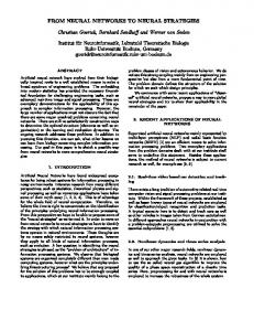
Orthogonal Search-based Rule Extraction (OSRE) for Trained Neural Networks: A Practical and Efficient Approach T. A. Etchells and P. J.G. Lisboa School of Computing and Mathematical Sciences Liverpool John Moores University, UK Abstract-There is much interest in rule extraction from neural networks and a plethora of different methods have been proposed for this purpose. We discuss the merits of pedagogical and decompositional approaches to rule extraction from trained neural networks, and show that some currently used methods for binary data comply with a theoretical formalism for extraction of Boolean rules from continuously valued logic. This formalism is extended into a generic methodology for rule extraction from smooth decision surfaces fitted to discrete or quantised continuous variables independently of the analytical structure of the underlying model, and in a manner that is efficient even for high input dimensions. This methodology is then tested with Monks’ data, for which exact rules are obtained and to Wisconsin’s breast cancer data, where a small number of high-order rules are identified whose discriminatory performance can be directly visualised.

Keywords: Rule extraction, neural networks. I. INTRODUCTION The current interest in the use of neural networks in medical applications has raised the important issue of explaining individual inferences by the network [1]. This is important from a practical point of view in order to properly verify and validate the neural network model, and potentially also from a legal standpoint as the doctrine of ‘learned intermediaries’ places on the clinician a responsibility to understand any inferences derived from the model. The contribution of the paper is threefold. First, to extend an effective current rule extraction algorithm, RULENEG [2], to 1-from-N coded categorical and ordinal datasets. Second, to present a mathematical formalism that underpins the proposed method. Thirdly, to illustrate the efficiency and effectiveness of the method with challenging benchmark data sets. This paper proposes a principled method to overcome common limitations in current ruleextraction models, meeting the requirements of accuracy in representing the decision inferences made by the network, together with computational efficiency to scale-up to high numbers of input dimensions. The latter is particularly important in medical applications as the variables are often categorical, which in 1-from-N coding leads to a proliferation of binary attributes.

An important reason for not using the model structure directly in rule extraction is that the simplest and most informative decision surfaces may require complex networks, while over-simple networks e.g. of minimal size after pruning, may block those surfaces by pushing the model configuration into what amounts to local minima in the space of decision surfaces [3]. This apparently surprising result means that simple models can get in the way of simple rules and is consistent with good practice in network design where the network complexity is controlled by appropriate regularization, rather than by cutting out nodes [1]. II. RULE EXTRACTION FROM NEURAL NETWORKS In general, rule extraction algorithms using neural networks fall into two categories, namely, blackbox, or pedagogical, and decompositional. Pedagogical rule extraction algorithms treat the network as a black box in that they are unconcerned with the internal structure of the network. Rather, the extracted rules reflect the relationship between the input variables and the outputs, without the need to scrutinise the behaviour of any nodes within the network [2], [4] & [5]. The main issue with pedagogical approaches is that they are generally exponential in their complexity. An example of a pedagogical algorithm that overcomes the burden of exponentiality is RULENEG by restricting the input space to that of the training data. RULENEG however is only applicable to data that is binary and not categorical, ordinal or continuous. Decompositional rule extraction algorithms directly interpret the response of each node in the network, sometimes assigning linguistic meaning to the nodes. Rules are extracted by analysing the activations of hidden and output nodes and the weights attached to them. Examples of decompositional rule extraction algorithms are found in [5], [6], [7] & [8]. Recently there has been renewed interest in approaches to rule extraction linked to the network structure, either by staging the rule extraction process using propositional variables [9], by setting out an explicit correspondence between standard neural networks and fuzzy-rule models [10], and

using recursive models to encode and grow decision trees [11]. These approaches have the merit of facilitating the introduction of prior knowledge into the model. Generic frameworks have also been proposed to link neural network architectures to logical rules and the management of uncertainty [12] & [13] and for simultaneous rule and feature extraction [14]. These methods for data-driven rule extraction with neural networks differ in their ability to generate and rank simple rules, whether the rules need to be pruned for overlaps or inconsistencies, and in scalability of speed and accuracy for large data sizes and dimensionality. A. Problems with the Decompositional Approach Decompositional approaches can fail accurately to derive the logic of the underlying decision surface. For example, consider a two layer Multilayer Perceptron (MLP) with two inputs and two hidden nodes and one output node. The hidden nodes are described as a function of input coordinates ( x, y ) ∈ [0,1] by h1 ( x, y ) = S (−5 x − 5 y + 7)

and

The decompositional approach substitutes the logic of the hidden nodes into the logic of the logic of the output nodes, i.e. output = ( x . y ). false = x . y ,

yet the network has a Boolean logic of XOR = xy ∨ xy

when the input domain is restricted to {0,1} . This example, albeit a somewhat pathological case brought about by the effect of large output node weights, nevertheless casts a shadow over the ability of the decompositional approach to consistently describe the logic of trained neural networks. The proposed method is pedagogical, therefore it applies to any smooth decision surface whether it has been generated from a neural network, or a multivariate linear model, or any other analytical expression. The method will be developed to scale well to high input dimensions and extended to apply to 1-from-N coded data. III A RIGOROUS FRAMEWORK FOR NONCLASSICAL LOGICS

h2 ( x, y ) = S (−5 x − 5 y − 1.5) with output ( x, y ) = S (20h1 ( x, y ) − 100h2 ( x, y ) − 6) . TABLE 1 THE RESPONSE OF EACH NODE OF THE NETWORK FOR BINARY INPUT VALUES.

x

y

h1

h2

output

1 1

1 0

0.05 0.88

0.00 0.00

0.01 1.00

0 0

1 0

0.88 1.00

0.00 0.18

1.00 0.01

From Table 1, the Boolean logic exhibited by the hidden nodes is h1 = x y and h2 = false .

Tsukimoto [5] developed a scalar, continuously valued algebra, represented by a multi-linear approximation to the decision surface, which it meets at the corners of a hypercube, where values of the input domain are restricted to the elements of the set {0,1} . Importantly, the scalar logic defines a linear vector space of non classical logics, whereby the function approximation generated by the network can now be seen to represent a well-defined logic in a metric space. This enables the identification of a Boolean logic for the function represented by the neural network. A. Multi-Linear Approximations to the Response Surface of Trained Neural Networks A multi-linear function is of the form n 2   f ( x1 , ... , xn ) = ∑  ai ∏ e(x j )  i =1  j =1  n

TABLE 2 THE BOOLEAN LOGIC OF THE OUTPUT NODE USING THE HIDDEN NODES AS INPUTS

h1 1 1 0 0

h2 1 0 1 0

output 0.00 1.00 0.00 0.00

Table 2 shows that the Boolean function that describes the logic of the output node in terms of the hidden nodes is output = h1 h2 .

where e( x j ) = x j or 1 − x j and ai are constants to be fitted to the neural network for binary values of n

the inputs.

Each product

∏ e(x ) j =1

j

is called an

‘atom’ as it represents a building block for the logic, specified by a corner of a unit hypercube in input space. The linear space spanned by the atoms of Boolean algebra is shown to be a Euclidean space [5].

For example a 2 input neural network, f ( x1 , x2 ) , can be approximated by the multi-linear function f ( x1 , x2 ) ≈ f (1,1) x1 x2 + f (1, 0) x1 (1 − x2 ) + f (0,1)(1 − x1 ) x2 + f (0, 0)(1 − x1 )(1 − x2 )

where xi ∈ [ 0,1] and the constants ai are generated

multi-linear functions all powers of x collapse to at most the linear term, i.e. x n = x . Boolean atoms are now seen to represent n

conjunctive forms ∧ e( xi ) , where e( xi ) = xi or i =1

xi and n is the number of variables in the input space.

from the output of the neural network f ( x1 , x2 ) from the substitution of either xi = 1 or 0. This expression is Lagrange’s 2 variable interpolating polynomial. Tsukimoto [5] showed that this function represents the continuously valued logic of the network, to which the closest Boolean logic, in the Euclidean sense, is shown to be obtained by rounding each coefficient ai to 1 or 0, corresponding to pegging the network response to a binary output at each of the logical atoms, i.e.

Atoms are by definition mutually exclusive, therefore their conjunctions with each other have the Boolean value false. Another important property of Boolean atoms is that the order (i.e. the number of terms) of the disjunction of adjacent atoms (next door neighbours) is always less that the order, or power of x, of the original atoms, due to the Boolean identity xy ∨ xy ≡ y , where y is any Boolean function.

1 (ai ≥ 0.5) ai =  . 0 (ai < 0.5)

C. Critique of the Multi-Linear Framework for Continuously Valued Logics Whilst the continuous valued logic framework readily generates optimal Boolean approximations to scalar-valued functions, it does not scale to networks with a large number of inputs, as there are 2n values to be calculated. In addition, if the input dimensionality is high then, as the Boolean atoms are of order the number of inputs, the simplification of the disjunction of all the atoms could be cumbersome even with powerful computer algebra systems. Furthermore, the ensuing Boolean expressions are likely to be of high order and therefore too complex to be comprehensible. Tsukimoto [5] proposes a polynomial algorithm that extracts low order rules, which have more information, from a network. However, the limitation of the algorithm is that it can only be applied to a network that has an output which is monotonically increasing. Whilst the output of an individual node is monotonically increasing with respect to its inputs, it is not generally true for a network of nodes with respect to the networks inputs. So, this amounts to a decompositional approach which applies the polynomial algorithm to each node in the network, extracting low order rules. As described in section II A, incorrect logic can result from a decompositional approach.

For example, if a 2 input network is written as the multi-linear function, then it’s nearest Boolean approximation is derived by the following process: f ( x1 , x2 ) ≈ 0.1x1 x2 + 0.9 x1 (1 − x2 ) − 0.1(1 − x1 ) x2 +0.85(1 − x1 )(1 − x2 ) → false ∨ x1 x2 ∨ false ∨ x1 x2 = x2

The approximation f ( x1 , x2 ) ≈ x1 (1 − x2 ) + (1 − x1 )(1 − x2 ) = (1 − x2 )

is the analytical representation of the Boolean logic represented by the smooth decision surface such as is generated by a neural network trained for a binary classification task. Clearly, the number of atoms in this multi-linear representation of a neural network increases exponentially with the number of inputs. B. Approximation of Scalar Algebras with Boolean Rules Tsukimoto’s algebra [5] is shown to be closed and consistent in the domain xi ∈ [ 0,1] under the Boolean operands AND, OR and NEGATION modelled with the following scalar expressions: x ∧ y → xy x ∨ y = x + y − xy x → 1− x .

This representation of Boolean functions does not proliferate polynomial expressions as in the space of

e.g.

x1 x2 x3 x4 ∨ x1 x2 x3 x4 = x2 x3 x4 .

D. Optimality of RULENEG and BIO-RE Under the Multi-linear Framework The methodology of RULENEG [2] and BIO-RE [4] are essentially the same, looping through each data point, then for each data point looping over the input variables stepwise negating each input and keeping a list of those inputs for which the negation changes the response of the network. Both algorithms apply this strategy for binary data, although they differ in the way that the Boolean

functions of the input variables that represent the inclass responses are simplified. RULENEG looks for changes in activation from each input to each step wise negated input (as described above) i.e. atomic neighbours. The BIORE algorithm employs simplification methods such as Karnaugh maps, algebraic manipulations or a tabulation method. In RULENEG, the stepwise negation is an algebraic manipulation applying the identity ( x ∧ y ) ∨ ( x ∧ y ) = y to simplify rules in disjunctive normal form. In this section the common algorithm of these two rule extraction methods is shown to produce rules for the region of the training data that are optimal in the sense of Tsukimoto’s multi-linear framework. A network of n inputs generates a multi-linear function with 2n terms. The space that is generated by the network’s input variables is normally much greater than that of the space occupied by the data that trained the network. The multi-linear terms (atoms) each represent distinct regions of the space and the sum of all the terms (regions) being the whole space. Hence evaluating the multi-linear terms (regions/atoms) that contain the data that trained the network reduce the problem from exponential, in terms of the number of inputs; to linear, in terms of training data. When the inputs of a neural network are restricted to {0,1} , the network surface spans the

pairing-up of atoms in the multi-linear approximation to the network response surface. In other words, RULENEG and BIO-RE are pragmatic and efficient methods to simplify the atomic representation of the underlying logic represented by the neural network when trained with binary data. Consequently, the rules extracted by these methods automatically satisfy Tsukimoto’s optimality criterion.

space of an n dimensional hyper-cube. Each vertex of the hypercube represents a Boolean atom and if the data is binary then the position vector of a vertex represents a possible binary data item, indeed a binary data item is a Boolean atom in vector form. If the output of the network for a binary data item is ≥ 0.5 then this atom is present in the disjunctive normal form of the logic for the network. By visiting each of the data items in the training data and evaluating the response of the network determines the active Boolean atoms in the space occupied by the data. Hence the Boolean atoms that are present in the disjunctive normal form of the logic of the network which optimally describe the behaviour occupied by the network in the subspace of the training data. If a data item (or atom) produces a ≥ 0.5 response from the network, we call this an active data atom. Contiguous input values where the network’s response remains in-class, represent atomic cells that factorise out of the disjunctive normal form as noted earlier. However, if the activation of the atoms does change from ≥ 0.5 to 2 whose variables are now binary and correspond to the quantisation x1,1 , x1,2 , x1,3 ,

, x1, m1 , x2,1 , x2,2 , x2,3

, x2, m2 , x3,1 , x3,2 , x3,3 … , xn ,1 , xn ,2 , xn ,3

, x3, m3 , xn, mn

where n is the number of variables in the original dataset and mi represents the quantisation of the ith variable. n

There are potentially 2 space, of the form e( x1,1 )e( x1,2 )e( x1,3 )

∑ mi i =1

Boolean atoms in this

e( x1, m1 )e( x2,1 )e( x2,2 )e( x2,3 )

e( x2, m2 )e( x3,1 )e( x3,2 )e( x3,3 ) … e( xn,1 )e( xn ,2 )e( xn,3 )

e( x3, m3 )

e( xn , mn )

where e( x) = x or x . However, the original ordinal data constrains the number and form of these Boolean atoms. This is due to the fact that only a subset of the binary vectors, hence Boolean atoms, actually represent the possible data items. These atoms form a restricted Boolean space such that the total number of possible Boolean atoms Nmax that represent valid data is given by n

Nmax= ∏ mi . i =1

∧x j ≠i

j

.

Every other Boolean atom is disallowed and it is readily shown that the disjunction of all the restricted Boolean atoms, within the restricted Boolean space, is a tautology, that is to say,

∨α m

i =1

i

a2 = 4 ≥ 0.5

= true ,