RESEARCH ARTICLES
Retrieval of forest phenological parameters from remote sensing-based NDVI time-series data C. Prabakaran*, C. P. Singh, S. Panigrahy and J. S. Parihar Space Applications Centre, Indian Space Research Organisation, Jodhpur Tekra, Ahmedabad 380 015, India
Uttara Kannada district has diverse forest types ranging from tropical evergreen to dry deciduous. This study used remote sensing-based NDVI time-series data from 1999 to 2007 to create the phenological curves and maps for every season and each phenological parameter was created using TIMESAT program. It was observed that evergreen forest sites are always followed by deciduous forest sites in all phenological events. The season starts by August and ends by June the following year in evergreen forests. In deciduous forests, the season starts by May and ends by March the following year. Evergreen forests have longer season than deciduous forests. Maximum temperature and rainfall have negative (r = –0.785) and positive (r = 0.502) correlation respectively with start of the season. However, maximum temperature has high positive correlation (r = 0.942) with leaf senescence. This article indicates that more studies on the phenology of natural vegetation will help to understand the responses of plants towards the changes in the climatic condition. Keywords: Climatic factors, forest phenology, remote sensing, time-series data. PHENOLOGY is the study of biological phenomena (e.g. leaf bud burst, flowering, leaf fall, etc.) that are controlled by environmental and climatic factors, and therefore considered as a sensitive biosphere indicator of climate change1. For plants, this means a study of morphological and reproductive phases that they pass through, such as bud bursting, leaf expansion, onset of flowering, fruiting, leaf colouring and leaf fall. Vegetation growth is influenced by climate. Phenological analysis of forest provides a potential tool to address critical questions related to modelling and monitoring of climate change. The effects of climate change are of immense significance on plant phenology. Vegetative phenology provides quantitatively detailed information on seasonality and cycle of leaf functioning and is vital for understanding the interactions between the biosphere and the climate2.
*For correspondence. (e-mail:
[email protected]) CURRENT SCIENCE, VOL. 105, NO. 6, 25 SEPTEMBER 2013
Understanding and predicting changes in phenology is necessary to infer the response of plants towards climatic variation. Meteorological and other parameters such as temperature, rainfall, day-length, relative humidity and soil moisture regulate the vegetative phenology. However, the control of climatic factors on plant phenology in tropical trees is not well understood3. The prediction of vegetation phenological variables such as start of foliage season (SFS), maximum of foliage season (MFS), optimal foliage/leaf senescence (OFS), end of foliage season (EFS), and length of foliage season (LFS) provides the information needed for the study of the effects of climate change on forest phenology. These phenological variables are measured from ground and extracted from remotely sensed data. Ground-measured phenological variables provide species-specific information with high temporal resolution, but lack a spatial component. In contrast, temporally frequent remotely sensed data provide a unique opportunity to estimate phenological variables at a range of scales from local to global. In addition, phenological variables extracted from remotely sensed data have the potential to characterize seasonal variation in the response of ecosystems to changes in climatic variables. In remote sensing studies of vegetation, various vegetation indices have been developed. However, the Normalized Difference Vegetation Index (NDVI) is the most popular and frequently used among them. NDVI, which is a normalized ratio of red and near infrared (NIR) spectral reflectance (NDVI = (NIR – RED)/(NIR + RED)), is determined by the degree of absorption by chlorophyll in red wavelengths, which is proportional to leaf chlorophyll concentration and by the reflectance of NIR radiation, which is proportional to green leaf density4. Remote sensing-based NDVI time series – SPOT-VGT, MODIS, AVHRR and MERIS – have been used by many researchers for leaf phenological research. Phenological pattern studies and foliage activity monitoring through NDVI help in understanding the dynamics of vegetation with regard to climate change impact, carbon sequestering and earth–atmosphere energy interaction5. In this study we focus on the leaf phenological parameters such as onset of season, maximum greenness, maximum leaf abscission, end of season and length of season. Deriving phenological parameters involves data smooth795
RESEARCH ARTICLES ening, filtering and curve fitting with fine-tuning of parameters using ground-based observations. The groundbased phenological observations in India are well studied. However, the remote sensing-based phenological dynamics as well as the techniques of parameter retrieval are not well established. Therefore, the present study was made to understand the technique of retrieval of parameters, its validation and role of climatic variables on the phenological changes. The objectives of the present study are: (i) retrieval of foliar phenological parameters using NDVI time-series data, (ii) preparation of phenological maps and (iii) establishing the relationship of climatic factors with plant phenology.
Materials and method Study area The district of Uttara Kannada (13°55′–15°31′Ν lat; 74°9′–75°10′E long.), comprising an area of 10,200 km2, lies on the west coast of India (Figure 1) and was selected for this study because of the availability of published ground records on the leaf phenology of two forest types6. The hill range of the Western Ghats runs parallel to the coast, rising to a little over 1000 m amsl. Maximum temperature ranges from 28.2°C to 33.7°C and the minimum temperature recorded varies from 19°C to 27°C. The mean temperature of this district lies between 25.4°C and 30°C. Annual total rainfall recorded in the district is 322 cm. Maximum rainfall is received in the month of July. Monsoon extends from June till September. Monsoon months experience less maximum temperature because of incessant rainfall. The natural forests are of evergreen/semi-evergreen type along the slopes, and secondary/moist deciduous towards the east of the ridge. Based on the annual rainfall and vegetation types, for this study the district was broadly divided into evergreen/semi evergreen zone and secondary/moist deciduous zone (Figure 1, Table 1). Remote sensing data and GIS techniques are good potential sources to study the Indian tropical forest resource assessment and monitoring7 and also to address the management concerns of the forest canopy cover8. Uttara Kannada district forest maps and Forest Resources Information System (FORIS) were also developed using various thematic layers by remote sensing and GIS techniques9.
rological Department (IMD) in the form of 1° × 1° gridded spatial images10,11. However, the rainfall data are available only for 2007; and the temperature data are available only till 2005 (Table 2).
Data filtering and curve fitting The published phenological records by Bhat6 (based on work carried out during 1983–1985) were used as a surrogate for ground-based information. The sampling locations (Figure 1 and Table 1) as marked by Bhat6 were registered and digitized for setting the parameters and validation of the results. SPOT-VGT NDVI product of 9 years (1999–2007) amounting to 324 bands (36 bands/ year) was loaded in TIMESAT ver. 3.02 (ref. 12). The TIMESAT program was used to get the NDVI profile of all sampling locations. TIMESAT implements three processing methods based on least-squares fit to the upper envelope of the NDVI data. The first method uses local polynomial functions in the fitting, and it can classified as an adaptive Savitzky–Golay filter. The other two methods which are not considered in this study are ordinary least-squares methods, where data are fit to model functions of different complexity. All three processing methods use a preliminary definition of the seasonality
Data used In this study, SPOT-VGT NDVI product of 9 years (1999–2007), 10-day composite with 1 km × 1 km spatial resolution has been used. The climatic data such as maximum temperature, minimum temperature, mean temperature and rainfall were obtained from India Meteo796
Figure 1. Map of Uttara Kannada district showing the broad vegetation types and location of sites. CURRENT SCIENCE, VOL. 105, NO. 6, 25 SEPTEMBER 2013
RESEARCH ARTICLES Table 1.
Some important characteristics of the study sites from two different vegetation zones in Uttara Kannada district
Species type
Evergreen/semi-evergreen
Location Population density (no. of trees/ha) Evergreen (%) Deciduous (%) Level of biotic disturbance
Secondary/moist deciduous
Chandavar
Mirzan
Nagur
Santgal
485
280
1536
888
338
388
279
585
50 50 High
37 63 Very high
66 34 Moderate
76 24 Low
26 74 High
18 82 High
24 76 High
47 53 Moderate
Table 2. Period January 1999–December 2007 30 years normal data 1999–2005 1999–2007
NDVI District climate normal Max T, Min T and Mean T Rainfall
f (t) = c1 + c2sin(ω t) + c3cos(ω t) + c4sin(2ω t) + c4cos(2ω t), where ω = 6π /N. The first three basis functions determine base level and interannual trend, whereas the three pairs of sine and cosine functions correspond to one, two and three annual vegetational seasons respectively. The fitting procedure always gives three primary maxima. In addition, secondary and tertiary maxima may be found. If the amplitude of the secondary maxima exceeds a certain fraction of the amplitude of the primary maxima, we have two annual seasons. For cases where the amplitude of the secondary maxima is low, the number of annual seasons is set to one. For cases in which the amplitude of the secondary maxima is comparatively large, the number of annual seasons is set to two. The pre-processing to remove the spikes and outliers was carried out by applying a median filter. Further, adaptive Savitzky–Golay filtering and curve fitting were used to deduce the phenological parameters. This method fits a quadratic polynomial f (t) = c1 + c2t + c3t2 for each data value yi, i = 1, 2, … , N, to all 2n + 1 points in the moving window and replaces the value yi with the value of the polynomial at position ti in the following equation n
∑ c j yi + j .
j =− n
To account for the negatively biased noise, the fitting is done in multiple steps. CURRENT SCIENCE, VOL. 105, NO. 6, 25 SEPTEMBER 2013
Bengle-Sugavi
Bidralli
Sonda
Data used
Parameter
(uni-modal or bi-modal) along with approximate timings of the growing seasons. The seasonality in the program is determined using data values (ti, Ii), i = 1, 2, …, N for three years by fitting a model function
Bhairumbe
Source SPOT-VGT NCC, IMD, Pune NCC, IMD, Pune NCC, IMD, Pune
Resolution 1 km/10 days composite District level/(1971–2000) 1°/daily 1°/daily
The result is a smoothed curve adapted to the upper envelope of the values in the time series. The width n (i.e. window size) of the moving window determines the degree of smoothing, but it also affects the ability to follow a rapid change. In TIMESAT, the width n can be set by the user because sometimes it is necessary to locally tighten the window. The adaption strength value (i.e. weights) can be provided in TIMESAT for setting the upper envelope. The phenological parameters (dates determined by the curve fitting) are not affected by these weights; however, the absolute NDVI value increases. To arrive at the window size for curve filtering, the number of envelope iterations and adaption strength value, a set of experiments was carried out based on the known phenological parameters of the sampling locations (two locations in tropical evergreen and two in tropical deciduous) in the study area. The other two locations in each forest category were used for validation of the results.
Extracting phenological parameters Seasonal data were extracted for each location. From the nine years data, eight seasons (n – 1) were extracted. The start and end of foliage season can be set from 0 to 1. By trial and error method we arrived at the value of 0.1, i.e. 10% of the distance from the left and right minimum values from the maximum value of the curve. Peak of the curve (100%) has been considered as maximum greenness of that season. Maximum leaf-fall rate was set to 0.5, i.e. 50% (inflection point) between the peak value and right side maximum value (Figure 2). Jönsson and Eklundh13 had also set the start and end of the season to 10% while studying South African phenology. Tuanmu14 used 20% as start and end of foliage season to extract the phenological metrics in his studies. From the curve fitting, the seasonality parameters were extracted and the composite dates were converted into normal dates. 797
RESEARCH ARTICLES Extracting images of seasonality parameters To generate images of seasonality parameters, e.g. SFS, a time window containing the season was defined. For each pixel the seasonality is established. The season falling in the time window is the desired one and the seasonality parameter is extracted for this season and written to an image file. The user is advised to make the time window large enough to allow for a certain variation in the start and end of the season over the processed area. The extraction of images is done using TSF_seas2img, a FORTRAN program which is an in-build algorithm provided in TIMESAT. The timings of seasons do not normally follow the calendar year. For example, a vegetation season may start in August, peak in December, and fall-off in April the following year. Therefore, the time window selection was carried out accordingly.
Impact of climatic variables on plant phenology For the study of relationship between the phenological parameters and climatic factors, deciduous forest site was taken for analysis. The pure pixels of Uttara Kannada deciduous forest were selected using Global Land Cover map (GLC2000)15 for the zonal statistical analysis. The mean phenological value for SFS and OFS was derived from the zonal analysis. Temperature and rainfall data of 14 days before from the mean date of SFS and OFS were extracted from the meteorological data. Seven-days moving average was calculated for each meteorological parameter.
Results and discussion Phenological parameters Phenological parameters such as start of the season, maximum greenness, peak leaf fall, end of the season and
Figure 2. Basic phenological parameters: (a) start of foliage season (left 10%), (b) end of foliage season (right 10%), (c) Stability of greenness (left 50% level), (d) Stability of leaf fall or optimal foliage senescence (right 50% level), (e) peak, (f) amplitude and (g) length of foliage season. 798
length of the season were extracted from SPOT-VGT NDVI multi-temporal data using TIMESAT. The number of annual seasons (n–1, i.e. eight seasons) was resolved using SPOT-VGT NDVI data for nine years. Window size for curve fitting was determined as 17. Number of envelope iterations was set to three and the adaption strength was set at five. The seasonality was found distinctly unimodal in nature for both categories of forest. The phenological curves were prepared for each sampling location (Figure 3).
Evergreen/semi-evergreen forests Nagur and Santgal have greater percentage of evergreen vegetation with low anthropogenic pressure; therefore, the NDVI value remains stable at the higher side throughout (≈ 75% of the total length of) the season. However, there was a distinct increase in NDVI during August (onset of greenness, i.e. start of the season), a peak during January and a decline which reaches a maximum by May the following year (peak leaf fall). The season ends in June. The NDVI increase can be attributed to the phenomenon of leaf flushing. Normally, the leaf initiation occurs in pre-monsoon dry period when the day length and temperature increase rapidly. This process ensures that young, photosynthetically competent leaves are in place when the monsoon rains begin. However, the satellite-based sensors are not able to detect the greenness at this stage, because NDVI varies with leaf area index and the concentration of chlorophyll, which is not sufficient enough to be detected. Moreover, cloud contamination during monsoon also plays spoilsport during start of the season. May is the transition period when the NDVI values decrease up to a certain limit and then start increasing slowly. In fact, in evergreen forests there is no distinct leafless period because of the phenomenon of ‘leaf exchange’, i.e. shedding of old leaves (during early dry season) is accompanied or immediately followed by bud burst and expansion of new leaves. In contrast to Nagur and Santgal, the other two locations, i.e. Mirzan and Chandavar are semi-evergreen in nature with more anthropogenic disturbances. The NDVI value does not remain stable due to semi-evergreen nature of the forest, with overstorey deciduous trees and understorey evergreen vegetation. However, there was a sharp increase in NDVI during June (onset of greenness, i.e. start of the season), a peak during November and a decline which reaches a maxima by February the next year followed by end of the season during April. The probable reason for the prolonged leaf fall season (two months compared to one month in the case of Nagur and Santgal) was the exposure of understorey evergreen vegetation during the overstorey deciduous vegetation leaf fall. CURRENT SCIENCE, VOL. 105, NO. 6, 25 SEPTEMBER 2013
RESEARCH ARTICLES
Figure 3. Phenological parameters retrieved from Savitzky–Golay curve fitting. Blue lines are NDVI temporal curve and orange lines are fitted curve.
Secondary/moist deciduous forests The moist deciduous vegetation in Bhairumbe, BengleSugavi and Bidralli exhibits a sharp increase in NDVI values from May, a peak during November and a decline which reaches a maxima by January the following year. CURRENT SCIENCE, VOL. 105, NO. 6, 25 SEPTEMBER 2013
The season ends in March. However, in Sonda the percentage of trees having evergreen characteristics is high (Table 1). Therefore, slightly different seasonality is observed here. Sonda witnesses as start of the season in June followed by peak in January. The peak leaf fall during March and end of season generally occur in April. 799
RESEARCH ARTICLES
(Contd…) 800
CURRENT SCIENCE, VOL. 105, NO. 6, 25 SEPTEMBER 2013
RESEARCH ARTICLES (Contd…)
Figure 4.
Spatial phenological calendar maps of Uttara Kannada district forest for the eight seasons (1999–2007).
As far as end of season is concerned, most of the years exhibit different dates due to different temperature conditions. However, these forests are found in the rainshadow regions and their phenology is also limited by the availability of rainfall. In the dry season, these species are found shedding their leaves to avoid water loss through evapotranspiration16.
Spatial phenological calendar maps Spatial phenological calendar maps of Uttara Kannada district (Figure 4) were prepared for each parameter and every year, and non-forest area was masked out from the spatial phenological maps using the Forest Survey of India (FSI) data17. The start of the season of Uttara Kannada district was observed between May and September. However, the early start of the season was detected during May in the CURRENT SCIENCE, VOL. 105, NO. 6, 25 SEPTEMBER 2013
eastern part of the district, which is largely deciduous forest type. Majority of the central and northwestern parts of the district exhibited a start of greenness between July and September. The land cover in these areas is dominated by evergreen and semi-evergreen forest. The onset dates for evergreen forest type were delayed compared to the deciduous forest type. As the altitude increases, the onset dates also lengthened. Delay of 4 weeks for start of leaf flushing for an evergreen species at higher altitude compared to lower attitude was reported by Shukla and Ramakrishnan18. Forest greenness in Uttara Kannada district reached its peak between October and February. In all phenological parameters deciduous forest type showed early dates than evergreen forests. Thereafter, the greenness started to decline. Maximum rate of leaf fall was observed between January and May. Deciduous forest type exhibited early maximum senescence during January and February. Dry 801
RESEARCH ARTICLES weather condition with low minimum temperature and less day length enhanced the high rate of leaf fall. The season ended between February and July. It was also observed that, when moving from east to west along the district, the end of senescence was delayed. Moreover, for the area where there was an early onset of greenness, the end of senescence was also detected earlier. The length of the season (growing period envelope) of this area extended from 180 to 360 days. However, the histogram of the growing period shows mean growing period from 240 to 300 days. However, deciduous forest has less growing period than that of evergreen forest.
Relationship between plant phenology and climatic factors The 7-day moving average of each climatic factor was correlated with the mean phenological dates of SFS and OFS, and it was found that the eight days lag of temperature (r = –0.785) and 13 days lag of rainfall (r = 0.502) from mean SFS have a significant correlation. But in case of OFS, four days lag from the mean OFS had high correlation (r = 0.9418). However, OFS did not have any correlation with rainfall, as there was no rainfall observed during the senescence period. All the data from eight seasons were pooled together for regression analysis. The stepwise linear regression analysis was done with the phenological dates of SFS and OFS against the climatic parameters. The regression equations for SFS and OFS are given below. SFS = 177.485 + 10.753 × Min T – 9.101 × Max T + 0.261 × rainfall, OFS = –366.143 + 12.271 × Max T. Minimum temperature and rainfall have positive relationship; and maximum temperature has a negative relationship with the initiation dates of SFS. Also, increasing maximum temperature pre-matures the peak senescence.
Conclusion This article retrieves the phenological parameters and spatial calendar maps for Uttara Kannada forest phenology from the SPOT-NDVI time-series data using TIMESAT program – Savitzky–Golay fitting method. Evergreen and deciduous forest species are observed with distinguishable phenological pattern. It was found that onset of greenness is early in case of deciduous forests, followed by evergreen forest. Also, length of the growing season of evergreen forest is higher than that of deciduous forest. Meteorological parameters play a crucial role in the phenology of forest trees, especially maximum temperature and rainfall. The extracted phenological variables from this study can be used as an important input to study of the impact of climate change on natural vegeta802
tion. This contemporary technology has enabled us to conduct a spatial and temporal study over a large area and suggests that more studies on the phenology of natural vegetation can help us understand the responses of plants towards the changes in the climatic condition. 1. Chambers, L. E., Evidence of climate related shifts in Australian phenology. In proceedings of the 18th World IMACS/MODSIM Congress, Cairns, Australia, 2009. 2. Arora, V. K. and Boer, G. J., A parameterization of leaf phenology for the terrestrial ecosystem component of climate models. Global Change Biol., 2005, 11, 39–59. 3. Borchert, R., Climatic periodicity, phenology, and cambium activity in tropical dry forest trees. IAWA J., 1999, 20, 239–247. 4. Tucker, C. J., Red and photographic infrared linear combinations for monitoring vegetation. Remote Sensing Environ., 1979, 8, 127–150. 5. Agrawal, S., Joshi, P. K., Shukla, Y. and Roy, P. S., SPOT VEGETATION multi temporal data for classifying vegetation in south central Asia. Curr. Sci., 2003, 84, 1440–1448. 6. Bhat, D. M., Phenology of tree species of tropical moist forest of Uttar Kannada district, Karnataka, India. J. Biosci., 1992, 17, 325– 352. 7. Roy, P. S., Dutt, C. B. S. and Joshi, P. K., Tropical forest resource assessment and monitoring. Trop. Ecol., 2002, 43, 21–37. 8. Rama Chandra Prasad, P., Nagabhatla, N., Reddy, C. S., Gupta, S., Rajan, K. S., Raza, S. H. and Dutt, C. B. S., Assessing forest canopy closure in a geospatial medium to address management concerns for tropical islands – Southeast Asia. Environ. Monit. Assess., 2010, 60, 541–553. 9. Udaya Lakshmi, V., Murthy, M. S. R. and Dutt, C. B. S., Efficient forest resource management through GIS and remote sensing. Curr. Sci., 1998, 75, 272–282. 10. Rajeevan, M., Bhate, J., Kale, J. D. and Lal, B., High resolution daily gridded rainfall data for the Indian region: analysis of break and active monsoon spells. Curr. Sci., 2006, 91, 296–306. 11. Srivastava, A. K., Rajeevan, M. and Kshirsagar, S. R., Development of a high resolution daily gridded temperature data set (1969–2005) for the Indian region, NCC Report, India Meteorological Department, 2008. 12. Jönsson, P. and Eklundh, L., TIMESAT – a program for analyzing time-series of satellite sensor data. Comput. Geosci., 2004, 30, 833–845. 13. Jönsson, P. and Eklundh, L., Seasonality extraction by functionfitting to time series of satellite sensor data. IEEE Trans. Geosci. Remote Sensing, 2002, 40, 1824–1832. 14. Tuanmu, M., Viña, A., Bearer, S., Xu, W., Ouyang, Z., Zhang, H. and Liu, J., Mapping understorey vegetation using phenological characteristics derived from remotely sensed data. Remote Sensing Environ., 2010, 114, 1833–1844. 15. Bartholome, E. and Belward, A. S., GLC2000: a new approach to global land cover mapping from Earth observation data. Int. J. Remote Sensing, 2005, 26, 1959–1977. 16. Singh, K. P. and Kushwaha, C. P., Paradox of leaf phenology: Shorea robusta is a semi-evergreen species in tropical dry deciduous forests in India. Curr. Sci., 2005, 88, 1820–1824. 17. SFR, India state of forest report. Forest Survey of India, Dehradun. 2009, pp. 159–162. 18. Shukla, R. P. and Ramakrishnan, P. S., Leaf dynamics of tropical trees related to successional status. New Phytol., 1984, 97, 697–706. ACKNOWLEDGEMENTS. We thank A. S. Kiran Kumar, Director, Space Applications Centre, ISRO, Ahmedabad for encouragement and support. We also thank Dr R. P. Singh, Head, EHD and Dr H. A. Solanki for their constant guidance. Also to the anonymous reviewers for critical comments which helped us to improve the manuscript. Received 15 April 2013; revised accepted 24 July 2013 CURRENT SCIENCE, VOL. 105, NO. 6, 25 SEPTEMBER 2013