374
Return Loss Validation of a Novel Cantor based Antenna using FIT and FDTD Vivek Dhoot
Dhirubhai Ambani Institute of Information and Commmunication Technology Gandhinagar, Gujarat, India Email:
[email protected]
Abstract-In this paper, return loss of a newly proposed cantor based multifractal multiband monopole antenna is analyzed using two numerical methods for validation. The Finite Integration Technique (FIT) and the Finite Difference Time Domain Method (FDTD) are used for analysis. The proposed antenna has multi band characteristics covering several wireless applications in Ultra Wideband (UWB) including WLAN 2 .4 GHz applications. A commercially available simulator CST (Based on FIT) and a MATLAB program based on FDTD method (Written as a simulator) are utilized for observing return loss of the proposed antenna. Then a resonance comparision is done which shows great analogy i.e. validates the result of one numerical method against another one.
Index Terms-FIT, FDTD, multifractal, multiband antenna, UWB.
I. INTRODUCTION The Return Loss is an important parameter in the de signing and development of an antenna. Return loss shows the resonances of an antenna where the power is maximally transmitted or received. So it is necessary to analyze the return loss with less amount of error and efficient approximation. This purpose is achieved by using numerical methods for modeling and simulation of an antenna. There are several numerical methods available nowadays. In most of the cases an antenna is modeled and simulated using one numerical method only. But the final return loss of the antenna is validated when it is fabricated and tested practically. Sometimes the return loss produced by simulation does not meet the return loss practically measured. Now the antenna can not be fabricated again and again to fulfill the requirements. So one solution for this problem is proposed here. To validate the return loss produced by one numerical method, another numerical method can be used. This provides less probability of mismatch be tween the simulated and measured results. Thus to accomplish the task, two numerical methods namely the Finite Integration Technique (FIT) and the Finite Difference Time Domain (FDTD) method are used. These are distinguished according to the procedure used for solving the Maxwell's equations [1] [3]. FDTD uses the differential approach and FIT uses integral approach to solve Maxwell's equations. The Finite Difference Time Domain Technique, as the name shows that it works on
Sanjeev Gupta
Dhirubhai Ambani Institute of Information and Commmunication Technology Gandhinagar, Gujarat, India Email: sanjeev�
[email protected]
the finite differences of the differentials [2], [3]. The Finite Integration Technique works on the finite sums of integrals [13], [14]. Basically all the modeling techniques are used to discretize the Maxwell's equations and then implement them appropriately into the computers to process these discretized equations and observe the solutions [4], [5]. Return loss a newly proposed antenna is analyzed. The multifractal compact antenna design is at prime nowadays. The main attraction of these antennas is the salient features provided by them like ease of integration, good amount of radiation and low cost of construction. Several multifractal geometries have been presented in literature [9]-[11]. The proposed antenna is based on multifractal cantor geometry presented by B. Manimegalai et al. in [6]. The cantor geometry has major advantage of having self affine geometry [12]. The antenna proposed in this paper is developed by the second iteration of the antenna proposed in [6]. The main advantage of the proposed antenna is that it resonates at five different frequencies and covers widebands in UWB range in second iteration only with a less complex design structure. II. THE FINITE INTEGRATION TECHNIQUE The finite integration technique also known as, FIT, was developed by Thomas A. Weiland in 1977. It is a numerical discretization approach used for solving Maxwell's equations in their integral form [13], [14]. In other words, it establishes a discrete reformulation of Maxwell's equations in their integral form, suitable for computers. It allows simulation of real-world electromagnetic field problems with complex geometries. The final updating matrix equations of the discretized fields are used for efficient numerical simulations. In addition, the basic algebraic properties of this discrete electromagnetic field theory allow to analytically and to algebraically prove conservation properties with respect to energy and charge of the discrete formulation and gives an explanation of the stability properties of numerical formulations in the time domain. The Maxwell's equations in their integral form are given as
978-1-4244-9799-7/11/$26.00 ©2011 IEEE
375
Faraday's Law
1
&A
-
E·ds=
J
oR
-
-·dA A at surface, aA is
(1)
Where, A denotes any open its boundary (a closed curve), dA and d""'s are the vectorial area and line element, respectively. Ampere's Law
1
&A
-
H . ds =
JA
( aDat ) . dA -
-
+J
-
(2)
Where, A denotes any open surface, aA is its boundary (a closed curve), dA and d""'s are the vectorial area and line element, respectively. Gauss's Law of Electricity
rD. i'A = rpdv (3) J&V Jv Where, V denotes any �en volume, aV is its boundary (a closed surface), dv and dA are the small volume and vectorial area element, respectively. Gauss's Law of Magnetism
rR · dA =0 J&V
(4)
Where, V denotes any o'pen volume, aV is its boundary (a closed surface), dv and dA are the small volume and vectorial area element, respectively. FIT usually represents an open boundary problem to a simply connected and bounded space region. The decomposition of the computational domain into a (locally) finite number of simplified cells is done such as tetra or hexahedra, under the premise that all cells have to fit exactly to each other as shown in Fig. 1.
The intersection of two different cells is either empty or it must be a two-dimensional polygon, a one-dimensional edge shared by both cells or a point. After discretization of the Maxwell's equations into finite sums, a matrix form is derived and represented in equations as follows:
1
&A
-
E.
-
-
ds =
rH- · ds = J&A A
J
oR - . dA
JA at
{:}
( aD ) . dA 7it + J
-
Ce =
{:}
d:::. b dt
(5)
--
Ch = -�
rD. iA = rpdv {:} Sb =0 J&V Jv
dd dt + j �
:::.
(6)
(7)
(8) C is the discrete curl operator, S is the discrete divergence operator, C is the dual discrete curl and S is the dual discrete divergence in dual grid approach [13]. III. THE FINITE DIFFERENCE TIME DOMAIN METHOD The Finite Difference Time Domain method is very old, impactive, accurate and easy to implement modeling method used for solving any electromagnetic problem. The FDTD method was presented by Kane Yee in 1966 [1]. The 3D FDTD method considers complete high frequency structure in 3 dimensions. This provides better observational region for an electromagnetic problem. The basic concept of this method is that it subdivides a complete computational space into small cells. 3D model of a high frequency structure is then analyzed according to these small grid cells. These cells are known as Yee cells [1]. FDTD updating equations are then derived for each cell. These updating equations of electric field and magnetic field for one cell are then used to update the electric and magnetic field values for the next cell. The procedure is then repeated corresponding to the Time Marching Algorithm [2], [4], [5]. The Maxwell's equations in differential form are given as: Ampere's law (9) Faraday's law
yo
�: : : :
x
-
aii
-
-
E = -Mat: + am E + Mi
(10)
Gauss's electric law (11) Gauss's magnetic law (12) Fig. 1.
Grid Cell Discretization
Here, E is electric field strength, D is electric field displace ment, H is magnetic field strength, B is magnetic flux density,
376
J
is electric current density, M is magnetic current density (virtual), Pe is electric charge density, Pm is magnetic charge density (virtual) and yo is the spatial del operator. € is material permittivity, J.L is material permeability, Je is conduction elec tric current density , Ji is impressed electric current density, e a is electric conductivity of the material, Me is conduction magnetic current density, Mi is impressed magnetic current density, am is magnetic conductivity of the material. For Determining derivatives of the electric and magnetic field components with respect to time and space, central difference formula or forward or backward difference formula is used. First or second order of these formulas are used generally. First order forward and center difference formulas are given as follows:ty, J.L is material permeability, Je is conduction electric current density , Ji is impressed electric current density, ae is electric conductivity of the material, Me is conduction magnetic current density, Mi is impressed magnetic current density, am is magnetic conductivity of the material. For Determining derivatives of the electric and magnetic field components with respect to time and space, central difference formula or forward or backward difference formula is used. First or second order of these formulas are used generally. First order forward and center difference formulas are given as follows: Forward Difference
/ (x)
=
f(x + �x) - f(x) �x
Central Difference
/ (x)
=
f(x + �x)
x
A novel multiband antenna is proposed in this paper. This antenna design is based on the multifractal cantor based geometry proposed by B. Manimegalai et al. in [6]. This antenna is developed on the basis of cantor set geometry and then some modifications are proposed to obtain better return loss. A. Cantor Geometry
An initiator of height H and width W is used to form a self similar object known as Cantor Set [6], [12]. Partitioning of the initiator (KO) provides three non overlapping segments with the removed middle segment. This procedure is repeatedly used for generation of consecutive iterations. Cantor fractal iterations are shown in Fig. 2.
W H
(a) Initiator
WI3
WI3
(13) (b) First Iteration
� f(x - �x)
2
IV. DESIGN OF ANTENNA
.
W/9
W/9
(14)
As presented in [2], [4], [5], the electric fields are sampled at 0, �t, 2�t, 3�t, . . ., n�t, time positions (Integer time steps) and the magnetic fields are sampled at (1I2)�t, (1+112) �t, . . ., (n+1I2)�t, time positions according to the dual grid approach (Half integer time steps) and are offset from each other by (�t/2). This time step satisfies the courant factor given in the form of CFL condition as
....
W/9
W/9
iii
+-----+
-
-
-
(c) Second Iteration Fig. 2.
Cantor Fractal Geometry
Iteration Function System (IFS), represented by self affine transformation, is used to describe it [6], [12]. The transfor mation of initiator into iterative layer is represented in matrix form as:
(15)
(18)
If a cubical cell is used then (16) Or generally