Reverse Engineering of XML Schemas to Conceptual Diagrams

Reverse Engineering of XML Schemas to Conceptual Diagrams Martin Neˇcask´y Department of Software Engineering Charles University, Prague, Czech Republic Email: [email protected]

Abstract It is frequent in practice that different logical XML schemas representing the same reality from different viewpoints exist. There is also usually a conceptual diagram modeling the reality independently of the viewpoints. It is important to keep the XML schemas and conceptual diagram consistent as they are both utilized for different purposes. In practice, this is however rarely the case. In this paper, we propose a reverse engineering method as a solution to this problem. We provide a semi– automatic algorithm that produces mappings of components of the XML schemas to components of the conceptual diagram. The method only provides suggestions for the mapping and manual participation of a domain expert is therefore required. Keywords: xml schema, conceptual model, reverse engineering. 1

Introduction

Without any doubt, XML is currently a de-facto standard for data representation. Its popularity is given by the fact that it is well-defined, easy-to-use and, at the same time, enough powerful. With a growing popularity of XML, there is also a growing need for effective methods and tools for designing XML data. In recent research, there has appeared several approaches that concentrate on so called forward engineering methods. These approaches usually apply the ER model (such as (Dobbie et al. 2000), (Mani 2004)) or UML class model (such as (Routledge et al. 2002) or (Bernauer et al. 2003)). They suppose designing a conceptual diagram of the problem domain first. After that, a representation in an XML schema language is derived automatically from the conceptual diagram. Usually, the applied XML schema language is XML Schema (Thompson et al. 2004). There exist recent surveys of this area, e.g. (Neˇcask´y 2008, Dom´ınguez et al. 2007, Bernauer et al. 2004). However, these approaches have not considered a crucial fact that information systems usually do not apply only one XML format but several (e.g. for sending purchase orders, browsing product catalogs, viewing sales reports, etc). These XML formats represent different views This paper was supported by the Grant Agency of Czech Republic (project 201/09/0990) and by the Ministry of Education of the Czech Republic (grant MSM0021620838). c Copyright °2009, Australian Computer Society, Inc. This paper appeared at the Sixth Asia-Pacific Conference on Conceptual Modelling (APCCM 2009), Wellington, New Zealand, January 2009. Conferences in Research and Practice in Information Technology (CRPIT), Vol. 96, Markus Kirchberg and Sebastian Link, Ed. Reproduction for academic, not-for profit purposes permitted provided this text is included.

X X X Y Y Y

458 3

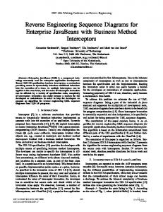
Figure 1: Purchase Request and Product Distribution XML Documents on the data in a system. It is natural since there are different groups of users who view the data (e.g. about customers, products or purchases) from different perspectives. Therefore, one concept can be represented in various XML formats in different ways. Example 1 demonstrates the situation. There are two XML documents. The XML document on the left demonstrates an XML format for purchase requests. The other represents an XML format for product sales reports. Both formats represent products, customers and purchases but in different XML structures, i.e. with different XML elements and attributes. Current approaches are not sufficient for designing such XML formats since they automatically translate a conceptual diagram into an XML schema. Therefore, this leads to augmenting a conceptual diagram for the needs of the corresponding XML format. It means enriching the diagram with syntactical constructs that model hierarchical structure (since XML is hierarchical in its nature), deciding whether a given part of the data should be represented as an XML element or attribute, etc. In the result, there is a separate conceptual diagram for each XML format. However, a conceptual diagram should be abstracted from the details of a concrete logical model (e.g. XML) and from a particular user view (e.g. XML format). In our previous work (Neˇcask´y 2007, 2008), we have developed a conceptual model for XML that overcomes the disadvantages of the existing approaches. We present the model briefly later in this paper. We can anticipate the main idea standing behind the model. It is a division of the conceptual modeling process to two steps. In the first step, a conceptual diagram describing a problem domain independently of its representation in various XML formats is designed. In the second step, required XML formats are designed on the base of the conceptual diagram. In this paper, we further extend our conceptual model with so called reverse engineering capabilities. We are motivated by a common situation in current information systems. As we have already discussed, there are usually

several XML formats each described by an XML schema. Usually, there also exists a UML class diagram or ER diagram, that describes the data at the conceptual level. This conceptual diagram is usually developed at the beginning of the development process but never used later. Consequently, the XML schemas are designed separately from the conceptual diagram and are therefore not explicitly mapped to the conceptual diagram. A common consequence is that the XML schemas are inconsistent with the conceptual diagram as well as with each other. This makes not only their design but also their maintenance harder (e.g. their evolution, change impact analysis, etc.). Suppose for example that we need to make a change in an XML schema, e.g. to remove an XML element declaration. This change can cause additional changes in other XML schemas as well to keep them consistent with each other. Today, it is necessary to make these additional changes manually which is time–consuming and error– prone. If we had a conceptual diagram and each XML schema was mapped to the conceptual diagram, we could propagate the change to the conceptual diagram first and from here to the other XML schemas automatically. This would automate the evolution process significantly. Reverse engineering of XML schemas, as we understand it in this paper, means to map existing XML schemas to an existing conceptual diagram. Because manual reverse engineering would be time–consuming and error– prone activity, we try to find a semi–automatic method, i.e. a method that is still performed by a domain expert but supported by a computer. Related Work. There exist several approaches to reverse engineering of XML schemas to UML class diagrams such as (Jensen et al. 2003)(Yang et al. 2006). There is also a recent survey in (Yu & Steele 2005). Their common characteristics is that they automatically translate an XML schema to a corresponding UML class diagram. However, the following facts, that we consider crucial for a reverse–engineering method to be successfully applicable in practice, have not been addressed yet: 1. UML class diagram modeling data at the conceptual level usually exists. Often, it is created during initial phases of the development process and rarely used later during system maintenance. 2. Several XML schemas describing different XML formats applied in the system exist. These formats reflect different perspectives of particular users. However, the XML schemas are mostly designed separately from the UML class diagram. If we apply existing approaches on a set of XML schemas, we get a set of separate UML class diagrams each being the result of an automated reverse engineering of the respective XML schema. These UML class diagrams are not interrelated neither with each other nor with the existing UML class diagram. Therefore, we can not utilize the reverse engineered UML class diagrams for, e.g. XML schema maintenance mentioned earlier. Contribution In this paper we try to overcome the described disadvantages of existing approaches to reverse engineering of XML schemas. For this purpose, we apply the Model-Driven Architecture (MDA) (Miller & Mukerji 2003) which considers two types of models. Platform– Independent Model (PIM) enables one to model data independently of any representation in any concrete data model. Platform–Specific Model (PSM) allows one to model representation of data modeled by the PIM diagram using constructs of a selected data model such as XML. In our approach, a PIM diagram is a UML class diagram that models data independently of its representation in XML, i.e. it is a conceptual diagram of the data. A PSM diagram is also a UML class diagram but models how the data is represented in a particular XML format. It models an XML schema of this XML format at the conceptual level. At this point, it is important to stress explicitly that

an XML schema and its PSM diagram represent a particular view on the system while the system is described independently of this view by the PIM diagram. The XML schema represents the view at the logical level, without any connection to the PIM diagram, while the PSM diagram represents the view at the conceptual level, with an explicit mapping to the PIM diagram. In this paper, we consider an existing PIM diagram and a set of XML schemas. We suppose that the XML schemas were designed manually without any explicit relationship to the PIM diagram. The XML schemas could also be imported to the system, e.g. because of needs of communication with other systems. This is a common situation in practice. Instead of automatic translation of each XML schema to a separate UML class diagram, we propose a semi–automatic method that maps components of the XML schemas to components of the PIM diagram. For each XML schema, the method constructs a PSM diagram that models the XML schema at the conceptual level and describes the semantics of its components in terms of the PIM diagram. The result is that the XML schemas are mapped to the PIM diagram. In other words, the PIM diagram integrates the XML schemas at the conceptual level. This facilitates maintenance of the XML schemas as well as other related tasks (e.g. their integration, data storage, etc.). For example, if a new user requirement appears, corresponding changes are made in the PIM diagram and are automatically propagated through the reverse engineered PSM diagrams to the XML schemas. A change can also be done in an XML schema or its PSM diagram and automatically propagated through the PIM diagram to the other XML schemas. Reverse engineering of XML schemas with an exploitation of an existing PIM diagram has not been studied yet to our best knowledge. This brings a new challenge of exploitation of semi-automatic schema mapping techniques ((Shvaiko & Euzenat 2005) (Chiticariu et al. 2007)) in reverse engineering techniques. 2

XML Schema

In this section we briefly describe the XML Schema language (Thompson et al. 2004) as it is an essential technology for this paper. It describes syntactical structure of XML documents, i.e. what XML elements and attributes can be used. XML Schema is an XML dialect, i.e. schemas are XML documents. An example XML schema is depicted in Figure 2. Since XML Schema provides a lot of constructs, we consider only basic ones to keep the complexity of the paper acceptable. The basic construct is element declaration. It is specified by an element element and declares elements with a given name. An element declaration has a simple or complex type. A simple type specifies that the declared elements contain text values. A complex type specifies that the elements have attributes and contain child elements. E.g., there is an element declaration with a name order-request at line 02 in Figure 2. It has assigned a complex type OrderRequest and declares elements order-request with attributes and child elements defined by the complex type. An element declaration with a name street has assigned a simple type string. It declares elements street containing a string value. Attribute declaration is specified by an element attribute and is used to declare attributes. It has a name and a simple type specifying values of the declared attributes. E.g., there is an attribute declaration with a name issue-date at line 13. Each simple or complex type is described by an XML Schema construct called type definition. It is specified by an element simpleType or complexType, respectively. A type definition has a name that identifies the type

01 02 03 04 05 06 07 08 09 10 11 12 13 14 15 16 17 18 19 20 21 22 23 24 25 26 27 28 29 30 31

Figure 3: PIM diagram

Figure 2: XML Schema Figure 4: Purchase PSM diagram 1

in the XML schema . In this paper we are interested only in complex types. E.g., there is a complex type definition OrderRequest at line 03. A complex type definition contains so called content model which defines child elements. It further contains a set of attribute declarations that define attributes. Even though XML Schema provides several constructs for defining content models, we consider only a construct sequence. It contains a list of element declarations and models an ordered sequence of child elements. It can also contain choice constructs. A choice contains one or more element declarations and models that only one of them can appear among child elements in a parent element. 3

Conceptual Model

In this section, we briefly introduce our MDA–based conceptual model for XML. For its full description see (Neˇcask´y 2008). 3.1

Platform–Independent Model

As a platform–independent model (PIM), we use UML class diagrams. Even though UML provides more constructs, we consider only classes with attributes and binary associations. As we mentioned in the introduction, a PIM diagram describes the problem domain independently of a representation of the domain in a concrete data model such as relational or XML. Example 1 Figure 3 shows a PIM diagram of a company. A class Purchase models purchases. It has attributes purchase-no and date modeling relevant purchase characteristics. An association connecting Purchase and Item models that purchases contain items. Associations can have labels that explicitly specify the semantics for the reader. For example, Purchase and Address are associated by two associations with labels ship and bill, respectively. 1

There can also be anonymous definitions but we omit them in this paper

3.2 Platform–Specific Model As a platform–specific model (PSM), we use UML class diagrams extended with some constructs for modeling XML specific details. A PSM diagram models a given XML format. There can be more PSM diagrams derived from a PIM diagram each modeling a separate XML format. The PSM diagram describes not only the structure of the format but also its semantics in terms of the PIM diagram since it uses its classes and associations. Example 2 Figure 4 depicts a PSM diagram derived from the PIM diagram depicted in Figure 3. It models the XML format for purchase requests demonstrated by the XML document depicted in Figure 1 on the left. A PSM diagram is a tree. It can be translated to a representation in an XML schema language (see (Neˇcask´y 2008)). Basic PSM building blocks are UML classes and directed binary UML associations. A PSM class Cpsm represents a PIM class C and specifies how instances of C are represented in the modeled XML format. Cpsm has the same name as C and zero or more attributes of C. For an attribute Attr, an expression Attr AS a specifies that Attr is assigned with an alias a. We use an alias if we want an attribute to be represented in the XML format with a name different from its original name. Cpsm further contains an ordered list of zero or more PSM associations going from Cpsm . This list is called content of Cpsm . A PSM association Apsm goes from a parent class to a child class. It represents a construction called nesting join that describes the semantics of Apsm in terms of components of the PIM diagram. We introduce nesting joins later in this section. Here, we anticipate that a nesting join specifies nesting of instances of PIM classes represented by the PSM classes connected by Apsm . A PSM class Cpsm , that represents a PIM class C, models that an instance of C is represented in XML documents as a set of XML attributes and sequence of XML elements. The XML attributes are modeled by the attributes of Cpsm . An attribute Attr models an XML attribute with a name given by an alias of Attr or name of Attr (if Attr

does not have an alias). The XML elements are modeled by the content of Cpsm . Let Apsm be a PSM association 0 in the content going to a PSM class Cpsm that represents 0 a PIM class C . Apsm models that the XML code representing an instance c0 of C 0 is contained in the XML code representing an instance c of C if c0 is nested in c by Apsm . Cpsm can have assigned a label called element label. It is displayed above Cpsm . If Cpsm has an element label l, the XML elements and attributes modeled by Cpsm are enclosed in an XML element named l. Otherwise, they are propagated to the closest ancestor with an element label. An existence of such an ancestor is ensured since each root PSM class must have an element label. PSM further contains constructs for modeling XML syntactic details. An attribute container can be contained in the content of a PSM class Cpsm and contains one or more attributes of Cpsm . It models that the attributes are represented as XML elements not attributes. A content choice can also be contained in the content of a PSM class Cpsm and models variants in the content of Cpsm . It contains two or more PSM associations going from Cpsm and specifies that only one of them can be instantiated for each instance of Cpsm . A structural representative Rpsm is a PSM class that inherits attributes and content of another PSM class Cpsm . Both Rpsm and Cpsm must represent the same PIM class. Rpsm can have its own element label. Example 3 Assume again the PSM diagram depicted in Figure 4. Its root P urchasepsm represents P urchase. It has an element label order-request. Further, it has an attribute date with an alias issue-date. The other attribute purchase-no of P urchase is not represented. The content of P urchasepsm contains a PSM association going to a PSM class Addresspsm and PSM association going to a structural representative of Addresspsm . A structural representative is displayed as a class but with a dashed line. The associations are followed by a content choice. It is displayed by a circle with an inner ’|’ and contains two PSM associations going to M essengerpsm and V anpsm . It specifies that each purchase has only a messenger or van but not both. Finally, there is a PSM association going to Itempsm . It nests items in corresponding purchases. The diagram also contains attribute containers. E.g., Addresspsm has its attributes street, postcode and city separated to an attribute container. An XML document depicted in Figure 1 on the left is an XML representation of a purchase as modeled by the PSM diagram in Figure 4. Because the root P urchasepsm has the element label order-request, the XML representation of the purchase is enclosed in an XML element order-request. Its attribute date with the alias issuedate specifies that a purchase date is represented as an XML attribute issue-date of order-request. The PSM association going to Addresspsm with the element label ship-addr specifies that a ship address is nested in the purchase. The XML representation of the ship address is modeled by Addresspsm . It is enclosed in an XML element ship-addr because of the element label. Similarly, the XML representation of a bill address is enclosed in an XML element bill-addr. Because the attributes of Addresspsm are separated to the attribute container, the XML elements ship-addr and bill-addr have child elements street, postcode and city. The PSM association going to Itempsm with element label ol specifies that items are nested in the purchase. An XML representation of each item is enclosed in an XML element ol. The PSM association going from Itempsm to P roductpsm specifies that each item has nested a purchased product. Because P roductpsm does not have an element label, the XML representation of the product, which is XML attribute product-code, is not enclosed in a separate XML element but propagated to the upper XML element ol.

3.3

Nesting Joins

Each PSM class represents a PIM class. It means that semantics of the PSM class is specified by the PIM class. In this section, we propose a formalism for specifying semantics of PSM associations. Informally, semantics of a PSM association specifies what child instances are nested in a given parent instance. Basically, semantics of a PSM association Apsm can be specified by a PIM association Apim . Assume that Apsm 0 goes from a PSM class Cpsm to a PSM class Cpsm where the PSM classes represent PIM classes C and C 0 , respectively. The semantics of Apsm can be specified by Apim if Apim connects C and C 0 . In that case Apsm nests an instance of C 0 in an instance of C if the instances are connected by Apim . Since PSM diagrams represent views on PIM diagrams, we need a more advanced mechanism to specify semantics of PSM associations. The first generalization discussed in this paper is specification of semantics by a path in a PIM diagram instead of PIM association. The principle is similar to the previous case since a PIM association can be comprehended as a path of length 1. Informally, a path goes from a PIM class C to a PIM class C 0 . If the semantics of a PSM association Apsm is described by this path, Apsm nests an instance of C 0 in an instance of C if the instances are connected by the path. We define paths in PIM diagrams formally in the following definition. Definition 1 A PIM path P is an expression C1 −· · ·−Cn where C1 , . . ., Cn are PIM classes and for each 1 ≤ i < n, there is a PIM association connecting Ci with Ci+1 . If there are two or more associations connecting Ci and Ci+1 , we need to distinguish the required association by its name l and write (l, Ci+1 ) instead of Ci+1 . We say that P goes from C1 to Cn . Cn is called terminal class of P . Consistency between a PIM diagram and derived PSM diagrams is ensured by the following definition. Definition 2 If a PIM path C1 −· · ·−Cn specifies the semantics of a PSM association Apsm , we say that Apsm represents the PIM path. Apsm can represent the PIM 0 path only if Cpsm represents C1 and Cpsm represents Cn . Formally, the semantics of a PSM association representing a PIM path is defined by the following definition. Definition 3 Let Apsm be a PSM association representing a PIM path C1 −· · ·−Cn . Let c1 and cn be instances of C1 and Cn , respectively. Apsm nests cn in c1 if cn ∈ c1 JC1 −· · ·−Cn K. c1 JC1 −· · ·−Cn K denotes a set that is defined recursively as follows: S ci JCi−. . .−Cn K = ci+1 ∈ci (Ci+1 ) ci+1 JCi+1−. . .−Cn K, cn JCn K ={cn } where ci (Ci+1 ) is a set of all instances of Ci+1 connected with ci by the respective PIM association. If cn ∈ c1 JC1 − · · ·−Cn K, we say that cn is accessible by P from c1 . Example 4 The semantics of all PSM associations depicted in Figure 4 can be specified by PIM associations depicted in Figure 3. For example, the PIM association named ship connecting PIM classes Purchase and Address specifies the semantics of the PSM association going from Purchasepsm to Addresspsm . On the other hand, there can be PSM associations whose semantics can not be described simply by a PIM association. Suppose for example a PSM diagram depicted in Figure 5 on the right. There is a PSM association going from Productpsm to Regionpsm . However, there is no PIM association in the PIM diagram in Figure 3 connecting Product and Region. We need to specify that the PSM association nests in each product a list of regions

from where the product was purchased. This semantics is specified in terms of the PIM diagram by a PIM path Product−Item−Purchase−(bill,Address)−Region. We further propose a generalization of PIM paths for describing semantics of PSM associations. This generalization is called nesting join. Suppose again a PSM association Apsm with semantics specified by a PIM path going from a PIM class C to C 0 . This semantics can also be interpreted as a grouping of instances of C 0 by Apsm . More precisely, instances of C 0 form a group if they are nested by Apsm in the same instance of C. Therefore, each instance of C has a nested group of instances of C 0 . This group is defined by Apsm . We can extend this mechanism to grouping instances of C 0 not only by its parent but also one or more ancestors. The best way to explain this is to show an example. Example 5 Suppose a PSM diagram depicted in Figure 5 on the left. There is a PSM class Supplypsm . It has ancestors Supplierpsm , Partpsm and ProductSetpsm . Supplypsm represents a PIM class Supply which models supplies of parts. Parts are supplied by suppliers. A product set is produced from supplied parts. For each supply, we therefore have its supplier, supplied part, and product set. In the PSM diagram, we want to model an XML structure where supplies are grouped by suppliers, parts and products sets. More precisely, supplies form a group if they have the same supplier, part and product set. To represent this grouping in the required hierarchical structure, the PSM association going from Supplierpsm to Partpsm must nest a part in a supplier if there is a supply of the part by the supplier. Further, the PSM association going from Partpsm to ProductSetpsm must nest a product set in a part, that is nested in a given supplier, if there is a supply of the part to the product set by the supplier. Finally, the PSM association going from ProductSetpsm to Supplypsm must nest a supply in a product set, that is nested in a given part and supplier, if the supply is supplied by the supplier and supplies the part to the product set. We can also say that a supply is nested in a product set in the context of a part and supplier. We use nesting joins to describe such semantics. A nesting join must specify a grouped PIM class (e.g. Supply), joined PIM classes (e.g. Supplier with Part, Part with ProductSet, or ProductSet with Supply, respectively), and PIM classes that form the context for the grouping (e.g. empty context for the former PSM association, Supplier for the second, and Supplier and Part for the other, respectively). In the rest of this section, we introduce nesting joins formally. Before this, we define some auxiliary terms. Definition 4 We say that a PIM path is direct if it does not contain the same PIM class twice or more times. The only exception is the beginning and end of the path. Definition 5 Let P be a PIM path. rev(P ) denotes P in the reversed direction. It goes from Cn to C1 through the same PIM associations as P . Now, we are ready to define nesting joins formally. Definition 6 A nesting join is described by an expression C P1 ,...,Pk [P → Q] C is a PIM class whose grouping is described by the nesting join. P1 , . . ., Pk are direct PIM paths that go from C to PIM classes that form a context for the grouping. P and Q are direct PIM paths that go from C. P and Q are called parent and child of the nesting join. The arrow between P and Q specifies an orientation of the nesting join. To simplify the expression, we can leave the starting C from P1 , . . ., Pk , P and Q, since they must start with C anyway.

Figure 5: Supplier Report and Product Distribution PSM Diagrams Consistency between a PIM diagram and derived PSM diagrams is ensured by the following definition. Definition 7 If a nesting join C P1 ,...,Pk [P → Q] specifies the semantics of a PSM association Apsm , we say that Apsm represents the nesting join. Let Apsm goes from a 0 PSM class Cpsm to Cpsm that represent PIM classes C 0 and C , respectively. Apsm can represent the nesting join only if the following conditions are satisfied: (J1) C and C 0 are terminal classes of P and Q, respectively (J2) if k > 0, there is a PSM association that goes to Cpsm and represents a nesting join C P1 ,...,Pk−1 [Pk → P ] This ensures that PIM classes that form the context of C P1 ,...,Pk [P → Q] are also represented in the PSM diagram as ancestors of the parent of Apsm . Formally, the semantics of a PSM association representing a nesting join is given by the following definition. Definition 8 Let Apsm be a PSM association representing a nesting join C P1 ,...,Pk [P → Q]. For each k-tuple p1 , . . . pk , where pi is an instance of the terminal class of Pi , Apsm nests an instance q of the terminal class of Q in an instance p of the terminal class of P if there is an instance c of C such that p ∈ cJP K, q ∈ cJQK, and ∀1 ≤ i ≤ k : pi ∈ cJPi K. We say that q is nested in p in the context of p1 , . . ., pk . Example 6 Assume again the PSM diagram depicted in Figure 5 on the left. As we explained before, its hierarchical structure represents grouping of instances of Supply. Therefore, we need nesting joins to specify the semantics of PSM associations forming this structure. The PSM association going from Supplierpsm to Partpsm nests in each supplier a list of supplied parts. Formally, it nests an instance part of Part in an instance supplier of Supplier if there exists an instance supply of Supply such that supplier ∈ supplyJ Supply−Supplier K and part ∈ supplyJ Supply−Part K. This semantics is specified by a nesting join Supply[Supply − Supplier → Supply − P art] We can also leave the grouped class Supply, i.e. we can write Supply[Supplier → P art] The PSM association going from Partpsm to ProductSetpsm nests in each part a list of product sets to which the part was supplied. Moreover, the superior supplier has to be considered, i.e. the part contains only the product sets to which it was supplied by the supplier. Such semantics is specified by





Figure 6: Supplier Report XML Documents

Supply Supplier [P art → P roductSet] Formally, for each superior instance supplier of Supplier, the PSM association nests an instance productset of P roductSet in an instance part of P art if there exists an instance supply of Supply such that supplier ∈ supplyJSupply − SupplierK, part ∈ supplyJSupply − P artK, and productset ∈ supplyJSupply − P roductSetK. In other words, it joins P roductSet instances with Supplier and P art instances on the described conditions and groups the result by Supplier and P art. The PSM association going from P roductSetpsm to Supplypsm nests in each product set a list of supplies supplied by the superior supplier and supplying the superior part. This semantics is specified by Supply Supplier,P art [P roductSet →] Two example XML documents modeled by this PSM diagram are depicted in Figure 6. The left–hand side XML document is for a supplier with number ’S1’ and the right– hand side is for a supplier with number ’S2’. We can see that both supplied the same part with number ’P121’. However, the part has nested in each XML document different product set depending on the superior supplier. This is modeled by the context of the PSM association going from P artpsm to P roductSetpsm . Example 7 We can also use longer PIM paths in nesting joins. Assume the PSM diagram depicted on the right hand side of Figure 5. The PSM associations in the diagram represent respectively the following nesting joins: P urchase[Item−P roduct → (bill,Address)−Region] P urchaseItem−P roduct [(bill, Address)−Region →] The former specifies that the PSM association going from P roductpsm to Regionpsm nests an instance region of Region in an instance product of Product if there exists an instance purchase of Purchase such that product ∈ purchaseJP urchase − Item − P roductK and region ∈ purchaseJP urchase−(bill, Address)−RegionK. Informally, it connects to each product a list of regions from where the product has been purchased. The latter specifies that the PSM association going from Regionpsm to P urchasepsm connects to each region the list of purchases from the region that purchase the superior product. We unify the proposed mechanisms for specifying semantics of PSM associations (i.e. PIM associations, PIM paths and nesting joins). We comprehend a PIM association as a PIM path of length 1. Further, we comprehend a PIM path P going from a PIM class C to C 0 as a nesting join C 0 [rev(P ) → C 0 ] Both are equivalent since P nests instances of C 0 in instances of C. In other words, it groups instances of C 0 and nests the groups to corresponding instances of C. This grouping is described by the nesting join.

Example 8 Assume the PSM diagram in Figure 4. The PSM association going from P urchasepsm to Addresspsm with an element label ship-addr represents a nesting join Address[(ship, P urchase) →] Formally, it nests an instance a of Address in an instance p of P urchase if there exists an instance a0 of Address such that p ∈ a0 JAddress − (ship, P urchase)K and a ∈ a0 JAddressK = {a0 }, i.e. a = a0 . Informally, it nests in each purchase its ship address. The other PSM associations represent the following nesting joins respectively: Address[(bill, P urchase) → ], M essenger[P urchase → ], V an[P urchase → ], Item[P urchase → ] and P roduct[Item → ]. 4

XML Schema Reverse Engineering

The conceptual model proposed in the previous section can be used for modeling XML schemas as follows. We first design a PIM diagram and model each XML schema as a PSM diagram derived from the PIM diagram. The PSM diagram can then be mechanically translated to an XML Schema representation. In this paper, we are interested in the reversed process that starts with one or more XML schemas. We suppose that a conceptual PIM diagram already exists and we need to construct PSM diagrams that model the XML schemas in terms of the PIM diagram. Since doing this manually would be time– consuming and error–prone task, we show how to semi– automate this process. We suppose XML Schema as a language for syntactical description of XML schemas. Formally, the problem is given as follows. We have an XML schema Sxml and a PIM diagram Spim . We need to construct a PSM diagram Spsm that models the same XML format as Sxml and is derived from Spim . In other words, PSM classes from Spsm must represent PIM classes from Spim and PSM associations from Spsm must represent nesting joins specified over components of Spim . We separate the process to two steps. In a first step a first approximation of the target Spsm is mechanically derived from the XML schema. We call the result of the first step initial PSM diagram. In a second step the first approximation is refined by mapping components of Spsm to components of Spim . We describe both steps in detail in the following subsections. There can be situations that go beyond the scope of the paper. First, we suppose that a given PIM diagram and XML schemas model the same data. If not, it can be impossible to fully map an XML schema to the PIM diagram since a required attribute, class or association can be missing. This requires a refinement of the PIM diagram which is not considered in this paper. Second, we suppose only basic constructions for mapping, i.e. mapping a PSM attribute/class to an equivalent PIM attribute/class and mapping a PSM association to an equivalent nesting join. However, there can be more complex situations that require, e.g. to map a concatenation of more PSM attributes to one PIM attribute. This situations are not therefore covered by this paper. On the other hand, it is only a technical problem to extend the proposed solution with such mapping constructs. Our solution can not automatically provide the right solution of the mapping problem. We only look for a good approximation. It means that we estimate a mapping of a given component of an XML schema to components of the PIM diagram. However, the final decision about the mapping is left to a domain expert. 4.1

Initial PSM Diagram Construction

The translation of Sxml to an initial PSM diagram starts with global element declarations in Sxml . Only those having assigned a complex type are considered. The transla-

Figure 7: Initial PIM Diagram tion continues recursively to declarations of their child elements. To simplify the algorithm for the purposes of this paper, we suppose that all complex types are defined globally in the XML schema (locally defined complex types can be transformed to global declarations by assigning auxiliary names). Moreover, we do not work with various simple types that can be defined with XML Schema constructs. We consider all of them as they were the basic XML Schema simple type string. Let E be an element declaration with a name l and complex type T . We need to translate E and T . Since, there can be more element declarations sharing T , it is possible that T has already been translated during the translation of another element declaration. Therefore, the translation of E depends on whether T has been translated or not. Formally, E is translated as follows: (E1) If T has not been translated yet, E is translated to a PSM class Cpsm with an element label l. The name of Cpsm is given by the name of T (because it is defined globally, it must have a name). Moreover, Cpsm is set as so called base class of T . T is translated as we describe in a while ((T1–3) below). (E2) If T has already been translated during the translation of another element declaration E 0 , it has a base 0 0 is the result of the translation of . Cpsm class Cpsm 0 E according to (E2). In that case E is translated to 0 a structural representative of Cpsm . The structural representative has an element label l. If T has not been translated yet, we need to translate its attribute declarations and content model. A declaration of an attribute A with a name l is translated to a PSM attribute of Cpsm with a name l. The content model of T can be defined by various XML Schema constructs. As we mentioned in Section 2, we consider only sequence. A sequence can contain element declarations and choice constructs. A choice construct can contain element declarations. The components of the content model of T are translated as follows: (T1) Element declaration E 0 with a name l and simple type T 0 is translated to a PSM attribute with a name l. The cardinality of the new attribute is set according to minOccurs and maxOccurs of E 0 . The attribute is placed into an attribute container assigned to Cpsm . If there are more sibling element declarations with a simple type, the resulting attributes are coupled into one attribute container. (T2) Element declaration E 0 with a complex type T 0 is translated to a PSM class or structural representative 0 Cpsm according to (E1–2). A PSM association Apsm 0 going from Cpsm to Cpsm is created. The values of minOccurs and maxOccurs of E 0 are used as the 0 minimal and maximal cardinality of Cpsm in Apsm . (T3) choice is translated to a content choice assigned to Cpsm . The element declarations in the choice are translated recursively according to (T1–2) but assigned to the content choice instead of Cpsm .

Example 9 Assume the XML schema depicted in Figure 2. It is translated to an initial PSM diagram depicted in Figure 7. There is one global element declaration order-request with a complex type OrderRequest. Because OrderRequest has not been translated yet, order-request is translated according to (E1) to a PSM class OrderRequestpsm with an element label order-request. Further, OrderRequest is translated. The attribute declaration issue-date is translated to a PSM attribute issue-date of OrderRequestpsm . The content model of OrderRequest is translated as follows. The element declaration ship-addr has a complex type Address and (T2) is applied. ship-addr is translated according to (E1) because Address has not been translated yet. The result is a PSM class Addresspsm with an element label ship-addr. A PSM association going from OrderRequestpsm to Addresspsm is created. The cardinality constraint of Addresspsm in the PSM association is 0..1. Within the scope of the translation of ship-addr, Address is translated. It has no attributes and its content model contains element declarations street, postcode and city with simple types. They are translated according to (T1) to an attribute container assigned to Addresspsm with PSM attributes street, postcode and city, respectively. The element declaration bill-addr has a complex type Address and (T2) is applied. Because Address has already been translated, bill-addr is translated according to (E2) to a structural representative of the base class of Address which is Addresspsm . The structural representative has an element label bill-addr. A PSM association going from OrderRequestpsm to the structural representative is created. The choice is translated according to (T3) to a content choice in OrderRequestpsm . The element declarations messenger and van are translated according to (T2) to PSM classes M essengerpsm and V anpsm with element labels messenger and van, respectively. The element declaration ol has a complex type OL and (T2) is applied. (E1) is further applied because the complex type has not been translated yet. A PSM class OLpsm is created with an element label ol. The declaration of the attribute product-code is translated to a PSM attribute product-code. The declarations of the elements price and quantity are translated according to (T1) to PSM attributes price and quantity in an attribute container assigned to OLpsm . 4.2

PSM Diagram Semantics Refinement

An initial PSM diagram captures structure of Sxml . However, we also need to describe semantics of Sxml in terms of the PIM diagram Spim . It means to map components of Sxml to components of Spim . A na¨ıve solution is to let a domain expert to map the components manually. However, this is an error–prone and time–consuming task. In this section, we propose an algorithm for semiautomatic mapping of Sxml to Spim . It is semi-automatic since it just provides with mapping suggestions but still requires a participation of a domain expert. In the first two subsections we describe complementary algorithms for measuring similarity of strings and PIM paths weighting. In the third subsection, we describe the mapping algorithm in detail. 4.2.1

String Similarity

We will need to compute the similarity between two strings s1 and s2 . We could utilize various widely known algorithms for measuring syntactical and semantical similarity (see (Shvaiko & Euzenat 2005) for their survey). For simplicity, we utilize only the longest common substring of s1 and s2 since advanced algorithms for mea-

01 weightPaths(PIMClass C, PIMClass C 0 , String[] S) 02 int[] result; 03 for each PIM path P going from C to C 0 04 result[P ] := w(P, S) 05 return result

Figure 8: PIM Path Weighting Algorithm suring string similarity are not in our main interest in this paper. The similarity between s1 and s2 is computed as l(s1 , s2 ) sim(s1 , s2 ) = max{l(s1 ), l(s2 )} where l(s1 , s2 ) denotes the length of the longest common substring of s1 and s2 and l(s) denotes the length of s. We will also need to measure the similarity between two sets of strings S1 and S2 . It is computed as a sum of pairwise similarities of strings from S1 with strings from S2 normalized by the number of pairs: P s1 ∈S1 ,s2 ∈S2 sim(s1 , s2 ) ssim(S1 , S2 ) = |S1 ||S2 | 4.2.2

PIM Paths Weighting

We will also utilize an auxiliary algorithm weightPaths that weights direct PIM paths going from a PIM class C to a PIM class C 0 . The algorithm is depicted in Figure 8. It has C and C 0 as parameters. The third parameter S is a set of strings that influences the weight of the PIM paths. A weight of a given PIM path P is a number from the interval (0, 1) (including 0 and 1). It decreases with the growing length of P and increases with the similarity of the labels of the PIM associations and names of the PIM classes along P with the strings from S. Formally, the weight of a given direct PIM path P = C1 − . . . − Cn is computed as follows: w(P, S) = (

n−1 X i=1

1 + ssim({ai , ci+1 }, S) 1 )∗ i 2n

where for each i ∈ [1, n], ci is the name of the PIM class Ci and for each i ∈ [1, n − 1], ai is the label of the PIM association connecting Ci and Ci+1 in P . 4.2.3

Semi–automatic Mapping Algorithm

In this section we propose a semi–automatic algorithm classMap that maps components of an initial PSM diagram Sxml to components of a PIM diagram Spim . The algorithm is depicted in Figure 11. We start by applying classMap on the root PSM class Sxml . It maps the root to a corresponding PIM class and follows recursively to the descendants. According to the classification proposed in (Shvaiko & Euzenat 2005), the proposed algorithm belongs to the class of structural schema–based mapping techniques that measure similarity of the schema components on the base of children in a combination with string based techniques. For an actual PSM class Cpsm from Sxml , classMap proceeds in the following steps: • Class Mapping Estimation computes a similarity of Cpsm with each PIM class C. The similarity is a combination of a similarity of names and attributes of both classes as well as a similarity of children of Cpsm with neighbors of C. Therefore, it does not use only basic syntactical similarity but also structural similarity of the neighborhood of Cpsm with the neighborhood of C.

01 attrSim(PIMClass C, PSMAttribute Attrpsm ) 02 int[][] result; 03 for each PIM attribute Attr 04 PIMClass C 0 := Attr.class; 05 int sim := sim(Attrpsm .name, Attr.name); 06 if C = C 0 07 result[Attr][.] := sim; 08 else 09 string labels[] := {Attrpsm .name}; 10 result[Attr] := weightPaths(C, C 0 , labels); 11 for each direct PIM path P going from C to C 0 12 result[Attr][P ] := result[Attr][P ] ∗ sim; 13 return result;

Figure 9: Attribute Similarity Algorithm • Class Mapping Specification is performed by the domain expert who selects a PIM class for mapping of Cpsm from the list of PIM classes ordered by their similarity with Cpsm computed in the previous step. • Association Mapping performs mapping of a PSM association going to Cpsm , if there is any. Since a 0 parent Cpsm of the PSM association as well as its child Cpsm are mapped to PIM classes C 0 and C, respectively, the algorithm offers the list of PIM paths connecting C 0 and C ordered by their weights (see weightPaths algorithm depicted in Figure 4.2.2). The domain expert selects the right PIM path from a list of the PIM paths ordered by their weights. From the selected PIM path, an equivalent nesting join is constructed for mapping of the PSM association. • Subtree Mapping performs mapping of attributes of Cpsm and recursive mapping of the subtree of Cpsm . Example 10 Figure 4 shows the resulting PSM diagram after applying classMap on OrderRequestpsm from the initial PSM diagram depicted in Figure 7. 0 , it must If Cpsm is a structural representative of Cpsm 0 represent the same PIM class as Cpsm (lines 02–05, Cpsm .pim denotes the PIM class represented by Cpsm ). Otherwise, the four steps are performed. In the rest of this sections, we describe each step in detail. (1) Class Mapping Estimation. The first part of the classMap algorithm (lines 06–15) estimates mapping of Cpsm . It measures a similarity of Cpsm with each PIM class C. First, it computes a string similarity of a name of Cpsm with a name of C and similarity of an element label of Cpsm with the name of C. The maximum of the two values is stored to initSim (line 08). Next, classMap estimates mapping of the PSM attributes in Cpsm and in attribute containers assigned to Cpsm (lines 09–11). It assumes that Cpsm is mapped to C. The estimation itself is computed for each PSM attribute Attrpsm of Cpsm at line 11 by calling attrSim depicted in Figure 9. attrSim takes C and Attrpsm as parameters and computes a 2-dimensional matrix called attribute similarity matrix. The matrix is computed as follows. Attrpsm can be mapped to any PIM attribute Attr. Attr can be an attribute of C or an attribute of another PIM class C 0 . In the former case, the similarity of Attrpsm with Attr is computed as a similarity of their names (line 07). In the latter case, the similarity is moreover influenced by direct PIM paths connecting C and C 0 . This corresponds to a natural intuition. Attrpsm is a PSM attribute of Cpsm . We consider that Cpsm is mapped to C. If Attrpsm is mapped to Attr of C 0 , Cpsm represents a join of C and C 0 . Therefore, there must be a direct PIM path connecting C and C 0 otherwise the join can not be performed. Because there can be more direct PIM paths connecting C and C 0 , we assign a weight to each of them by calling weightPaths (line 10) with parameters C, C 0 and {Apsm .name}. The weight of a given

0 01 childSim(PIMClass C, PSMClass Cpsm ) 02 int[][] result; 03 for each PIM class C 0 0 04 int sim := max(sim(Cpsm .name), C 0 .name), 0 sim(Cpsm .label, C 0 .name)); 0 0 05 string labels[] := {Cpsm .name, Cpsm .label}; 06 result[C 0 ] := weightPaths(C, C 0 , labels); 07 for each direct PIM path P going from C to C 0 08 result[C 0 ][P ] := result[C 0 ][P ] ∗ sim; 09 return result;

Figure 10: Child Similarity Algorithm direct PIM path P increases with a decreasing length of P and with a growing similarity of names and labels along P with the name of Attrpsm . The resulting similarity of Attrpsm with Attr for a given PIM path P is the weight of P multiplied by the string similarity of the names of Attrpsm and Attr (line 12). attrSim returns the similarity of Attrpsm with each PIM attribute Attr for each direct PIM path connecting C and C 0 where C 0 is the PIM class of Attr. Note that . at line 07 denotes an empty PIM path and is added to suit the structure of the result. The algorithm classMap does not consider the whole attribute similarity matrix for C and Apsm to estimate the mapping of Cpsm . It uses only the maximal value in the matrix (line 11) which is added to the variable attrSim. The whole matrix is used later to suggest mapping of attributes to the domain expert. Finally, classMap estimates mapping of children of Cpsm (lines 12–14). It considers that Cpsm is mapped to 0 C. The estimation of a mapping of a given child Cpsm is computed by childSim depicted in Figure 10. It has C 0 and Cpsm as parameters and returns a 2-dimensional ma0 trix called child similarity matrix. Cpsm can be mapped to any PIM class. For an actual PIM class C 0 , the sim0 ilarity of Cpsm and C 0 is measured as follows. First, 0 the similarity of the name and element label of Cpsm 0 with the name of C is computed (line 04) and stored to sim. Second, PIM paths connecting C and C 0 are weighted by weightPaths with parameters C, C 0 and 0 0 .label} (line 06). This corresponds .name, Cpsm {Cpsm 0 is a child of Cpsm . Cpsm to a natural intuition. Cpsm 0 is mapped to C (consideration). Therefore, Cpsm can be 0 mapped to C if there is a PIM path connecting C and C 0 . There can be more such PIM paths. The weight of a given PIM path P increases with a decreasing length of P and with a growing similarity of names and labels along 0 P with the name and element label of Cpsm . Finally, we multiply the weight of a each PIM path connecting C and C 0 by sim (lines 07–08). childSim returns the similar0 ity of Cpsm with each PIM class C 0 for each direct PIM path connecting C and C 0 . The result of childSim is utilized by classMap at line 14. Only its maximum is considered and is added to the variable childSim. The whole matrix is used later for mapping PSM associations. The estimated similarity of Cpsm with C is computed as an avg of initSim, attrSim and childSim (line 15). Example 11 Assume classMap applied on OrderRequestpsm . The first part of the algorithm estimates mapping of OrderRequestpsm by computing its similarity with each PIM class. We show how the similarity of OrderRequestpsm with P urchase is computed. Similarity of the name, resp. element label, of OrderRequestpsm with the name of P urchase is computed first and the maximum of both is taken. The result is 0.08 since their common substring has length 1. Next, the algorithm estimates mapping of the attributes of OrderRequestpsm . For each of the attributes, the at-

01 classMap(PSMClass Cpsm ) 0 02 if Cpsm is structural representative of Cpsm 0 03 Cpsm .pim := Cpsm .pim; 0 04 Cpsm .name := Cpsm .name; 05 return; 06 int[] estimatedSim; 07 for each PIM class C 08 int initSim := max(sim(Cpsm .name, C.name), sim(Cpsm .label, C.name)); 09 int attrSim := 0; 10 for each Attrpsm ∈ Cpsm .attrs 11 attrSim := attrSim + max(attrSim(C, Attrpsm )); 12 int childSim := 0; 0 13 for each Cpsm ∈ Cpsm .childClasses 0 14 childSim := childSim + max(childSim(C, Cpsm )); 15 int estimatedSim[C] := initSim+attrSim+childSim ; 1+size(Cpsm .attrs)+size(Cpsm .children) 16 show PIM classes ordered by estimatedSim in descending order; 17 user selects a candidate C for mapping of Cpsm ; 18 Cpsm .pim := C; 19 if Cpsm is not a root 20 Apsm := PSM association going to Cpsm ; par 21 Cpsm := Cpsm .parentClass; par 22 C par := Cpsm .pim; 23 string labels[] := {Cpsm .name, Cpsm .label}; 24 weights := weightPaths(C par , C, labels); 25 show PIM paths going from C par to C ordered by weights in descending order 26 user selects a PIM path P from the list for mapping of Apsm ; 27 Apsm .pim := C[rev(P ) → C]; 0 28 for each Cpsm ∈ Cpsm .childClasses 0 29 classMap(Cpsm ); 30 for each Attrpsm ∈ Cpsm .attrs 31 attrMap(Attrpsm );

Figure 11: Class Mapping Algorithm tribute similarity matrix is computed by attrSim with a consideration that OrderRequestpsm is mapped to Purchase. The matrix contains a field for each PIM attribute Attr and each direct PIM path going from P urchase to the PIM class of Attr. Assume the matrix for the PSM attribute issuedatepsm . We show the computation of the similarity of issue-datepsm with the following three PIM attributes: • date of P urchase: sim(issue-date, date) = 0.40 is computed and line 07 is applied. • completion-date of P roductSet: sim(issue-date, completion-date) = 0.33 is computed and lines 09–12 are applied. weightPaths with parameters P urchase, P roductSet and string issue-date is called. It finds each direct PIM path going from P urchase to P roductSet and computes its weight. There are several PIM paths. For example, the weight of P urchase − (ship, Address) − (ship, Supply) − P roductSet is 0.34. The resulting similarity of issue-datepsm with completion-date for this PIM path is therefore 0.33 ∗ 0.34 = 0.11. All other PIM paths have a lower weight and are not therefore considered for the estimation. • supply-date of Supply: Analogously, we get 0.21. The similarity of issue-datepsm with other PIM attributes is insignificant. We return back to classMap. The algorithm takes only the maximal value 0.40 from the matrix, i.e. the mapping of issue-datepsm to the PIM attribute date of P urchase is considered. The variable attrSim summarizing the maximal similarities of the attributes of OrderRequestpsm with PIM attributes is therefore increased by 0.40.

P urchase Supply P roductSet

issue-date 0.40

ship-addr 0.74

bill-addr 0.74

messenger 0.75

van 0.75

ol 0.07 (bi,Ad)-(bi,Su)

da

(sh,Ad)

(bi,Ad)

Me

Va

0.46

0.74

0.74

0.38

0.35

0.07

su-da

(sh,Ad)

(bi,Ad)

(sh,Ad)-(sh,Pu)-Me

(sh,Ad)-(sh,Pu)-Va

(sh,Ad)-Re

0.33

0.45

0.45

0.30

0.29

0.08

co-da

Su-(sh,Ad)

Su-(bi,Ad)

Su-(sh,Ad)-(sh,Pu)-Me

Su-(sh,Ad)-(sh,Pu)-Va

Pr

init 0.08

est 0.50

0.08

0.40

0.08

0.28

Table 1: Evaluation of OrderRequestpsm Mapping Estimation After the estimation of mapping of the attributes of OrderRequestpsm , the algorithm classMap estimates mapping of the children of OrderRequestpsm . It com0 putes for each child Cpsm of OrderRequestpsm the child similarity matrix by calling childSim (line 14) with a consideration that OrderRequestpsm is mapped to P urchase. The matrix contains a field for each PIM class C 0 and direct PIM path going from P urchase to C 0 . Assume the computation of the child similarity matrix for the child Addresspsm with the element label ship-addr. childSim computes the similarity of Addresspsm with each PIM class C 0 for each PIM path going from P urchase to C 0 . An interesting PIM class is Address. childSim computes the string similarity of the names of Addresspsm and Address which is 1 (line 04). The similarity of the element label of Addresspsm with the name of Address is lower. Further, PIM paths going from P urchase to Address are weighted by weightPaths with parameters P urchase, Address and strings ’address’ and ’ship-addr’. There are two such PIM paths: P urchase − (ship, Address) and P urchase − (bill, Address) with weights 0.74 and 0.68, respectively. The string ’ship-addr’ influences the weight of the former because there is a label ship along the path which has non-zero similarity with ’ship-addr’. The weights are then multiplied by sim = 1. The similarity of Addresspsm with other PIM classes is insignificant. After the matrix for Addresspsm is computed, we return back to classMap where we take only the maximal value from the matrix, i.e. 0.74. Finally, the estimated similarity of OrderRequestpsm with P urchase is computed. The result is depicted in Table 1 in the last column (see Example 12 for details). Example 12 Table 1 shows the estimated similarity of OrderRequestpsm with PIM classes P urchase, Supply and P roductSet in the last column est. These PIM classes have the highest similarity with OrderRequestpsm . For each PIM class, we show the maximal value from the attribute similarity matrix for the attribute issue-datepsm . We also show the corresponding PIM attribute for which the similarity was computed2 . For example, the column (Supply,issue-date) shows the maximum from the attribute similarity matrix for issuedatepsm and Supply. It was computed for the PIM attribute supply-date of Supply. We further show the maximal value from the child similarity matrix for each child of OrderRequestpsm . We show the corresponding PIM path for each value. For example, the cell (Supply, messenger) shows the maximal value from the child similarity matrix for the child M essengerpsm and PIM class Supply. It also shows the PIM path for which the value was computed, i.e. Supply − (ship, Address) − (ship, P urchase) − M essenger. Table 2 shows the estimated similarity of the PSM class OLpsm with PIM classes Item and Address. The similarity with other PIM classes is insignificant. It shows that we can estimate the similarity even though the name and element label of the PSM class have nothing in common with the names of the PIM classes. (2) Class Mapping Specification. The second part of classMap (lines 16–18) performs the mapping of Cpsm 2 PIM paths and attributes in the table are abbreviated – for each step and attribute only the first two characters are shown

Item Address

product-code 0.64

price 0.5

quantity 0.25

Pr.pr-cd

un-pr

am

0.33

0.30

0.14

postcode

Su.un-pr

init 0.00

est 0.35

0.00

0.19

Table 2: Evaluation of OLpsm Mapping Estimation with a participation of the expert. It shows the list of PIM classes ordered by their estimated similarity with Cpsm (line 16) in descending order. The expert selects a PIM class C (line 17) and Cpsm is mapped to C (line 18). This completes the mapping of Cpsm . Example 13 After the estimation of mapping of OrderRequestpsm in Example 11, we show the list of all PIM classes ordered by their estimated similarity with OrderRequestpsm . The first three PIM classes are shown in Table 1. The expert selects P urchase. OrderRequestpsm is therefore mapped to P urchase. (3) Association Mapping. The third part of the classMap algorithm (lines 19–27) performs the mapping of the PSM association Apsm going to Cpsm if Cpsm 0 is not a root. Let Apsm go from Cpsm . We need to find a nesting join that describes the semantics of Apsm . 0 is mapped to a PIM class C 0 We already have that Cpsm and Cpsm to C. We need a direct PIM path going from C 0 to C as the base of the nesting join. The right PIM path must be selected by the domain expert. The algorithm only suggests suitable possibilities by weighting the PIM paths (line 24). Afterwards, the expert selects a PIM path P from the list of PIM paths ordered by their weights (lines 25–26) and Apsm is mapped to a nesting join C[rev(P ) → C] (line 27). Furthermore, it can be necessary to add a context to the nesting join. We describe this possibility later in Section 4.2.4. Example 14 We have OrderRequestpsm mapped to P urchase. Assume that we have its child Addresspsm with the element label ship-addr mapped to Address. We need to map the PSM association going from OrderRequestpsm to Addresspsm . The algorithm weights direct PIM paths going from P urchase to Address by calling weightPaths with parameters P urchase, Address and strings ’address’ and ’shipaddr’. The PIM paths were already weighted during the estimation of mapping of OrderRequestpsm in Example 11. We can therefore utilize the results. The algorithm shows the PIM paths ordered by their weight in descending order. The expert selects the path P urchase − (ship, Address) and the PSM association is consequently mapped to Address[(ship, P urchase) → ]. If the associations connecting P urchase and Address were distinguished by labels with the same similarity with ’address’ and ’ship-addr’, the PIM paths would have the same weight and we could not suggest the right mapping. (4) Subtree Mapping. Finally, classMap maps the PSM attributes of Cpsm to PIM attributes and child PSM classes of Cpsm to PIM classes (lines 28–31). Each child is mapped recursively by classMap (line 29). Each attribute is maped by an algorithm attrMap (line 31) depicted in Figure 12. It maps a PSM attribute Attrpsm in Cpsm or in an attribute container assigned to Cpsm . Cpsm

01 attrMap(PSMAttribute Attrpsm ) 02 C := Attrpsm .class.pim; 03 sim := attrSim(C, Attrpsm ); 04 show an ordered list of PIM attributes, the order of A is given by the maximal value in sim[A] (descending order); 05 user selects a PIM attribute Attr to be mapped to Attrpsm ; 06 Attrpsm .alias := Attrpsm .name; 07 Attrpsm .pim := Attr; 08 C 0 := Attr.class; 09 if C C 0 0 10 PSM class Cpsm is created; 0 0 11 Cpsm .psm := C 0 ;Cpsm .name := C 0 .name; 0 12 move Attrpsm to Cpsm ; 13 PSM association Apsm is created; 14 Apsm .parent := Apsm .class; 0 15 Apsm .child := Cpsm ; 16 show PIM paths going from C to C 0 ordered by sim[Attr] in descending order; 17 user selects a PIM path P for mapping to Apsm ; 18 Apsm .pim := C 0 [rev(P ) → C];

Figure 12: Attribute Map Algorithm was mapped with C in the previous part. attrMap starts with computing the attribute similarity matrix for Attrpsm and C (line 03). The matrix was computed during the estimation of mapping Cpsm and can be reused. The algorithm shows an ordered list of PIM attributes (line 04) in the descending order. The order of a PIM attribute Attr is given by the maximal value in sim[Attr]. The expert selects a PIM attribute Attr from the list and Attr is mapped with Attrpsm . If Attr is from C, we are done. If Attr is not from C but another PIM class C 0 , Attrpsm can not stay with its PSM class Cpsm because a PSM class representing C can have only attributes of C. We therefore create a new PSM 0 class Cpsm representing C 0 (lines 10–11) and Attrpsm is 0 0 moved to Cpsm (line 12). Cpsm must be added as a child of Cpsm . Therefore, a PSM association Apsm is created 0 with Cpsm as parent and Cpsm as child. Apsm must represent an appropriate nesting join. Therefore, we need to determine an appropriate PIM path P going from C to C 0 . P is selected by the domain expert from the list of PIM paths ordered by their weight in sim[Attr] (lines 16–17). Finally, Apsm is mapped to the nesting join C 0 [rev(P ) →]. Example 15 Assume that the PSM class OLpsm from the initial PSM diagram was mapped to the PIM class Item and we are mapping its PSM attribute productcodepsm . attrMap gets the attribute matrix similarity for product-codepsm and Item. It was computed during the estimation of mapping of OLpsm . The algorithm shows the list of PIM attributes ordered by their maximal estimated similarity with product-codepsm . The PIM attribute product-code of the PIM class P roduct is the most similar PIM attribute to product-codepsm as shown in Table 2 in the cell (Item,product-code). The expert selects product-code to be mapped to product-codepsm . Because product-code is from P roduct and not Item, a child PSM class P roductpsm mapped to P roduct is created and product-codepsm is moved here. Moreover, a PSM association going from OLpsm to P roductpsm is created. attrMap displays the list of PIM paths going from Item to P roduct ordered by their weights. The user selects Item − P roduct and the new PSM association is mapped to P roduct[Item →]. 4.2.4

Setting Class Context

0 Assume a PSM association Apsm whose parent Cpsm rep0 resents a PIM class C and child Cpsm represents C. The

algorithm classMap automatically maps Apsm to a nesting join C[P → C] where P is a PIM path going from C to C 0 . The nesting join specifies that an instance c of C is nested in an instance c0 of C 0 if c0 ∈ cJP K, i.e. C instances are joined with C 0 instances and grouped by C 0 . However, this semantics can be wrong because it can be necessary to add a context to the nesting join. Since it is very hard to determine the context automatically, we need a domain expert to decide. It should be as easy as possible for the domain expert. We propose the following procedure. After the semiautomatic mapping, the expert selects a non-root PSM class Cpsm representing a PIM class C. There is a PSM association Apsm going to Cpsm . Apsm represents a nesting join C[P → C]. The expert can add PIM classes represented by one or more ancestors of the parent of Cpsm to the context of the nesting join. To satisfy the conditions (J1) and (J2) introduced in 00 Section 3.3, if an ancestor Cpsm is considered, each PSM 00 class on the path from Cpsm to the parent of Cpsm must be considered too. Therefore, it is enough when the domain expert specifies a number of the ancestors that should be considered. Let k denote this number. For each of the ancestors, we need to add to the context the right PIM path going from C to the PIM class represented by the ancestor. Moreover, we also need to change the nesting joins represented by the PSM associations connecting the ancestors because the conditions (J1) and (J2) introduced in Section 3.3 must be satisfied. Formally, let C1,psm , . . ., Ck+2,psm be PSM classes such that Ck+2,psm = Cpsm and Ci,psm is the parent of Ci+1,psm for each i ∈ [1, k + 1]. Let Ci,psm represent a PIM class Ci for each i ∈ [1, k + 2] (Ck+2 = C). Let A1,psm , . . ., Ak+1,psm denote PSM associations where Ai,psm goes from Ci,psm to Ci+1,psm for each i ∈ [1, k + 1] (Ak+1,psm = Apsm ). Let Ai,psm represent a nesting join Ci+1 [Pi → Ci+1 ] where Pi is a PIM path going to Ci for each i ∈ [1, k + 1]. Finally, we suppose that for each i ∈ [1, k] the following conditions are satisfied: (C1) Pi contains a step which is the PIM class C, i.e. Pi = Pi,1 − C − Pi,2 (Pi,1 and Pi,2 can be empty), (C2) Pi+1,2 = rev(Pi,1 ) − Ci+1 where rev(P ) denotes P in the reversed direction (we put Pk+1,2 = Pk+1 ). If (C1–2) are not satisfied, the context can not be set. Each PIM path C − Pi,2 determines a PIM path that we need to put to the context. We therefore need to add the PIM paths P1,2 , . . ., Pk,2 to the context of the nesting join represented by Apsm (= Ak+1,psm ). The nesting joins represented by A1,psm , . . ., Ak,psm must be updated as well to satisfy the conditions (J1) and (J2). For each i ∈ [1, k] we need Ai,psm to represent a nesting join C[Pi,2 → Pi+1,2 ] instead of Ci+1 [Pi,1 − C − Pi,2 → Ci+1 ]. We show that the semantics described by both nesting joins is the same. The former nests an instance ci+1 of Ci+1 in an instance ci of Ci if the following condition (S1) is satisfied: (∃c ∈ JCK)(ci+1 ∈ cJC − Pi+1,2 K ∧ ci ∈ cJC − Pi,2 K) i.e. if there is an instance c of C such that ci+1 is accessible from c by the PIM path C − Pi+1,2 and ci is accessible from c by C − Pi,2 . The latter nests ci+1 in ci if the following condition (S2) is satisfied: ci ∈ ci+1 JCi+1 − Pi,1 − C − Pi,2 K i.e. if ci is accessible from ci+1 by Ci+1 −Pi,1 −C −Pi,2 . We show that (S1) and (S2) are equivalent. Assume that (S2) is satisfied for ci+1 and ci . It is equivalent to (∃c ∈ JCK)(c ∈ ci+1 JCi+1 −Pi,1 −CK∧ci ∈ cJC −Pi,2 K)

i.e. (S2) is satisfied if and only if there is an instance c of C such that c is accessible from ci+1 by Ci+1 − Pi,1 − C and ci from c by C − Pi,2 . This is further equivalent to (∃c ∈ JCK)( ci+1 ∈ cJC − rev(Pi,1 ) − Ci+1 K ∧ ci ∈ cJC − Pi,2 K ) because if c is accessible from ci+1 by Ci+1 − Pi,1 − C then ci+1 must be accessible from c by the reversed PIM path C − rev(Pi,1 ) − Ci+1 . Because (C2) is satisfied, we can change rev(Pi,1 ) − Ci+1 with Pi+1,2 and we get (S1). Therefore, we have that (S1) is equivalent with (S2). Now, we can set the required context and ensure that the conditions (J1) and (J2) from Section 3.3 are satisfied. We set Apsm to represent a nesting join C P1,2 ,...,Pk,2 [Pk+1,2 → C] and for each i ∈ [1, k] we set Ai,psm to represent C P1,2 ,...,Pi−1,2 [Pi,2 → Pi+1,2 ] Example 16 We demonstrate the proposed technique on a simple example. Assume the PSM diagram depicted on the left side of Figure 5. It was reverse engineered from an XML schema that we do not display. Its components were mapped to components from the PIM diagram in Figure 3 by classMap. The ancestors of Supplypsm are joined by PSM associations that represent nesting joins P art[Supply − Supplier → ], P roductSet[Supply − P art → ] and Supply[P roductSet → ], respectively. However, these joins do not describe the true semantics of the PSM associations. The true semantics is that supplies are considered in the context of suppliers, parts and product sets as we showed in Example 6. Therefore, the domain expert selects the PSM class Supplypsm and puts k = 2 to specify that Supply instances are not grouped only by P roductSet but also by the two ancestors P art and Supplier. We can easily verify that the conditions (C1–2) are satisfied. Both paths Supply − Supplier and Supply − P art contain a step Supply and (C1) is therefore satisfied. We have the following P1,1 = ., P1,2 = Supplier; P2,1 = ., P2,2 = P art; P3,2 = P roductSet where rev(.) − P art = P2,2 and rev(.) − P roductSet = P3,2 and (C2) is therefore satisfied as well. We can therefore update the nesting joins represented by the PSM associations according to the proposed technique as follows (respectively): Supply[Supplier → P art] Supply Supplier [P art → P roductSet] Supply Supplier,P art [P roductSet →] 5

Conclusions

We studied reverse engineering of XML schemas. We supposed a set of XML schemas and an existing conceptual diagram. We proposed a semi–automatic method that finds semantic interrelations between the XML schemas and the conceptual diagram. Currently, we are developing a tool for testing the proposed method in practice. We plan to extend the proposed algorithms with parameters for tuning them to fit real scenarios. It will be also necessary to further expand some technical details of the algorithms. We presented only a part of the conceptual model. The full model, that was proposed in (Neˇcask´y 2008), contains some technical extensions that allow to model more advanced XML features and therefore need to be considered for reverse engineering as well. Further, some more advanced algorithms for measuring not only syntactical but also semantical similarity of strings could be utilized. Last but not least is an optimization of the proposed algorithms.

References Bernauer, M., Kappel, G. & Kramler, G. (2003), Representing XML Schema in UML - An UML Profile for XML Schema, Technical report. Bernauer, M., Kappel, G. & Kramler, G. (2004), Representing XML Schema in UML - A Comparison of Approaches, in N. Koch, P. Fraternali & M. Wirsing, eds, ‘ICWE’, Vol. 3140 of Lecture Notes in Computer Science, Springer, pp. 440–444. Chiticariu, L., Hern´andez, M. A., Kolaitis, P. G. & Popa, L. (2007), Semi-Automatic Schema Integration in Clio, in C. Koch, J. Gehrke, M. N. Garofalakis, D. Srivastava, K. Aberer, A. Deshpande, D. Florescu, C. Y. Chan, V. Ganti, C.-C. Kanne, W. Klas & E. J. Neuhold, eds, ‘VLDB’, ACM, pp. 1326–1329. Dobbie, G., Xiaoying, W., Ling, T. & Lee, M. (2000), ORA-SS: An Object-Relationship-Attribute Model for Semi-Structured Data, Technical Report TR21/00, Dpt. of Computer Science, National University of Singapore. ´ RuDom´ınguez, E., Lloret, J., P´erez, B., Rodr´ıguez, A., bio, A. L. & Zapata, M. A. (2007), A Survey of UML Models to XML Schemas Transformations, in B. Benatallah, F. Casati, D. Georgakopoulos, C. Bartolini, W. Sadiq & C. Godart, eds, ‘WISE’, Vol. 4831 of Lecture Notes in Computer Science, Springer, pp. 184–195. Jensen, M. R., Møller, T. H. & Pedersen, T. B. (2003), ‘Converting XML DTDs to UML diagrams for conceptual data integration’, Data Knowl. Eng. 44(3), 323– 346. Mani, M. (2004), EReX: A Conceptual Model for XML, in Z. Bellahsene, T. Milo, M. Rys, D. Suciu & R. Unland, eds, ‘XSym’, Vol. 3186 of Lecture Notes in Computer Science, Springer, pp. 128–142. Miller, J. & Mukerji, J. (2003), MDA Guide Version 1.0.1, Object Management Group. http://www.omg.org/docs/omg/03-06-01.pdf. Neˇcask´y, M. (2007), XSEM - A Conceptual Model for XML, in J. F. Roddick & A. Hinze, eds, ‘Fourth Asia-Pacific Conference on Conceptual Modelling (APCCM2007)’, Vol. 67 of CRPIT, ACS, Ballarat, Australia, pp. 37–48. Neˇcask´y, M. (2008), Conceptual Modeling for XML, PhD thesis, Charles University. http://kocour.ms. mff.cuni.cz/˜necasky/dw/thesis.pdf. Routledge, N., Bird, L. & Goodchild, A. (2002), UML and XML Schema, in X. Zhou, ed., ‘Australasian Database Conference’, Vol. 5 of CRPIT, Australian Computer Society. Shvaiko, P. & Euzenat, J. (2005), ‘A Survey of SchemaBased Matching Approaches’, J. Data Semantics 6, 146–171. Thompson, H. S., Beech, D., Maloney, M. & Mendelsohn, N. (2004), XML Schema Part 1: Structures (Second Edition), W3C. http://www.w3.org/TR/xmlschema-1/. Yang, W., Gu, N. & Shi, B. (2006), Reverse Engineering XML, in J. Ni & J. Dongarra, eds, ‘IMSCCS (2)’, IEEE Computer Society, pp. 447–454. Yu, A. & Steele, R. (2005), An Overview of Research on Reverse Engineering XML Schemas into UML Diagrams, in ‘ICITA (2)’, IEEE Computer Society, pp. 772–777.