They have been used for simulating arbitrary 3D media as well as for development of ... The new EM tools provide full triaxial tensor measurement, in addition to ...
PIERS Proceedings, Cambridge, USA, July 5–8, 2010
390
Review of 3D EM Modeling and Interpretation Methods for Triaxial Induction and Propagation Resistivity Well Logging Tools S. Davydycheva1 and M. A. Frenkel2 1
3DEM Consulting, Texas, USA EMGS Americas, Texas, USA
2
Abstract— The 3D electromagnetic (EM) modeling and inversion techniques for the geological formation evaluation have been experiencing significant progress since the early 90s. There are three main 3D EM numerical techniques: finite-difference (FD), finite element (FE), and integral equation (IE). They have been used for simulating arbitrary 3D media as well as for development of 3D inversion-based interpretation of well log data acquired by the conventional and new-generation logging tools. We present a brief review of these three techniques as to their ability to simulate and interpret the new-generation of triaxial tensor wireline and logging-whiledrilling (LWD) measurements. The new EM tools provide full triaxial tensor measurement, in addition to the conventional axial measurement, when the formation is excited by an axial zdirected magnetic dipole transmitter, and the response of axial receivers is analyzed. Due to full 3D sensitivities, the new tools allow significantly enhanced formation resistivity interpretation. We present synthetic logs for four different new-generation tools: both triaxial induction and directional propagation resistivity LWD tools. We also consider new features in the new tool responses and discuss various post-acquisition processing techniques. These approaches allow to better visualize tool responses and enable efficient application of fast stable inversion schemes for resistivity interpretation. 1. INTRODUCTION
At least five new EM logging tools have been introduced in the last decade. In addition to the conventional axial ZZ measurement, they provide triaxial measurements, i.e., XX, XY , XZ, Y X, Y Y , Y Z, ZX, and ZY components (notation used: transmitter direction, receiver direction) that allow performing enhanced geological formation interpretation. However, extracting the formation geometry and properties out of the new tool data requires application of advanced 3D modeling and interpretation methods. 3D EM numerical modeling and inversion lately experienced significant progress. Three basic numerical techniques have been known to simulate EM measurements: the finite-difference (FD), the finite element (FE) and the integral equation (IE) methods. These techniques have been successfully applied to 3D modeling and interpretation of conventional resistivity logging [2]. In this paper, we review these techniques based on their ability to handle new-generation triaxial measurements, leaving aside the material related to the conventional EM logging tools. 2. NEW-GENERATION TENSOR RESISTIVITY MEASUREMENTS
In a vertical well with horizontal bedding, there is no coupling between vertical transmitters and transverse receivers and vice versa. Coupling only exists between transmitters and receivers of the same orientation. Any azimuthal asymmetry (dipping beds, dipping anisotropy, fractures, faults, asymmetric invasion zones, etc.) generates cross-terms XY , XZ, Y X, Y Z, ZX, and ZY . Two different concepts of triaxial induction measurements have been developed. Fig. 1(a) presents a simplified scheme of single-spacing tool 3DEX, including triaxial transmitter and receivers [16]. This tool is operating at ten frequencies ranging from 20 to 220 kHz. To reduce effects caused by the borehole, the invaded zone, and the tool eccentricity, the Multi-Frequency Focusing (MFF) method was introduced. It is based on calculation of a linear combination of 3DEX data acquired in the main and bucking receivers at two or more frequencies. The processed data can be interpreted using a uniform-medium model [16]. This approach is fast, but it leads to a reduction of the spatial resolution of anisotropy interpretation using 3DEX data. Spatial resolution of anisotropy interpretation is improved via the application of raw log data inversion. For example, the rapid inversion of 3DEX logs can be used to accurately determine the parameters of both invaded and uncontaminated zones [12]. The rapid inversion method also demonstrates the potential for substantially reducing computing time by partitioning the 2D inverse problem into a sequence of smaller 1D problems, thereby enabling the delivery of interpretation in run times comparable to run times for other familiar well-site deliverables.
Progress In Electromagnetics Research Symposium Proceedings, Cambridge, USA, July 5–8, 2010
391
To expand the operational range of 3DEX technology for use in wells drilled with very conductive waterbased muds, it was proposed logging 3DEX in combination with a galvanic tool and using 2D/3D inversion-based interpretation procedures [13]. Such an approach enables the determination of the formation resistivity anisotropy using 3DEX in boreholes with diameter ≤ 12 in., muds Rm ≥ 0.02 Ωm, and a relatively deep invasion of up to 18 in. Another concept implies multi-spacing triaxial measurements. The new tool (RtScanner, Fig. 1(b)) includes six balanced triaxial arrays [9]. This tool’s short spacings allow high spatial resolution, whereas the longer spacings and relatively low frequencies (13 and 27 kHz) enable high depth of investigation. Data symmetrization and rotation techniques allow separation of the borehole effect from the effects of dipping bed boundaries and the formation anisotropy, resulting in enhanced sensitivity to wanted formation properties [6]. Separation of the invasion zone effect from the formation response requires full 3D inversion [1]. New-generation LWD propagation resistivity measurements used for geo-steering purposes are also based on the multi-frequency, multi-spacing tilted [5, 15] or transverse [11] antenna concept. These tools take advantage of the tool rotation, providing directional measurement — as a ratio (or attenuation and phase shift) of the voltages measured at two positions of the tilted or transverse antenna, up and down. Such a measurement provides high sensitivity to dipping anisotropy, dipping bed boundaries and other azimuthal asymmetries. Transmitters’ and receivers’ configurations of two directional LWD tools, Azimuthal Deep-reading Resistivity (ADR [5]) and PeriScope [15], are depicted in Figs. 1(b) and 1(c), respectively. A detailed review of these tools is given in [21]. Full 2D or 3D inversions of directional resistivity LWD measurements are not yet common. Instead, the trial-and-error forward modeling is used to interpret 2D or 3D data [15]. 3. NUMERICAL MODELING METHODS: FE, FD AND IE
In FD and FE approaches, Maxwell’s differential equations with respect to the EM field (or its potentials) are discretized on a FD or FE mesh or grid. This leads to the resulting system of linear equations with respect to the approximate EM field/potentials, which is typically solved iteratively. The grid cells in the FD approach (which is nothing but a particular case of the FE approach) are typically conformal to the coordinate system; in Cartesian coordinates the grid boxes are rectangular blocks. This allows for relative simplicity of the FD numerical implementation. In the FE approach the grid elements may have almost arbitrary shapes (prisms, tetrahedrons, etc.). This apparent flexibility allows modeling non-trivial shapes, but it is counterbalanced by a nontrivial and usually time-consuming construction of the finite elements themselves. This is why the FD method is used more commonly than the FE method.
(a)
(b)
(c)
Figure 1: (a) Configuration of transmitters and receivers in two triaxial induction and two directional LWD resistivity tools (only long spacings of Periscope are shown); (b) 1D, (c) 2D FD models of the tools and the geological formation; the tool trajectory coincides with z-axis; transmitters and receivers are shown: (b) ADR; (c) PeriScope; the solid/dotted cyan lines depict primary/dual Lebedev subgrids.
PIERS Proceedings, Cambridge, USA, July 5–8, 2010
392
(a)
(b)
(c)
Figure 2: ADR synthetic response to the 85◦ -dipping layered 1D formation: (a) 125-kHz, (b) 500-kHz and (c) 2-MHz directional response of T1-R2 pair. A thin vertical line signifies the bed boundary.
3.1. The FD Method
Most FD software developers use the so-called staggered Yee FD grid (named after Yee, who introduced it in 1966), which was initially designed for isotropic media. The different components of the FD electric field and of the FD current density are determined at different edges of the grid boxes, and the different components of the FD magnetic field — at different faces of the grid boxes. Such a grid produces coercive approximation i.e. the current conservation law is satisfied. However, such a staggered grid does not easily allow applying the general anisotropic Ohm’s law, J = σE, with arbitrary non-diagonal conductivity tensor σ connecting all components of the current density J and the electric field E taken at the same spatial points. Recently, many authors have extended the Yee approach to arbitrary anisotropic media (see [19, 20, 14] among others). They use interpolation to obtain the different components of J and E at the same spatial points. This may lead to a loss of the current conservation property and, in the presence of the arbitrary dipping anisotropy, to the appearance of “parasitic” currents on the FD grid that may significantly reduce the accuracy of the FD scheme. When applying straightforward interpolation, the ingoing and outgoing grid currents (in those grid cells where the anisotropy tensor is non-diagonal) may not be equal anymore, since the differential identities curl grad ≡ 0 and div curl ≡ 0 may be broken for the interpolated fields on the FD grid. Circumventing this difficulty requires special efforts. This may result in inefficiently dense and large FD grids. Another approach to handle the arbitrary dipping anisotropy on the FD grid is the so-called Lebedev grid [7, 8]. It includes a combination of two (in the 2D case) or four (in the 3D case) subgrids-Yee grids shifted in space with respect to each other so that all the components of the electric field Ex , Ey and Ez , and the electric current density, Jx ,Jy and Jz are determined at the same spatial nodes. The Lebedev grid provides the current conservation property automatically and allows simple implementation of the anisotropic Ohm’s law. Moreover, even in trivial isotropic media the Lebedev grid demonstrates the FD error cancellation property at medium interfaces and at grid domain boundaries, which allows for a reduced grid domain size and density compared to the standard Yee grid. We illustrate this statement on an example of synthetic directional ADR response. Fig. 1(b) depicts a vertical cross-section of 1D 85◦ -dipping layered medium. We consider the synthetic ADR tool “moving” through this medium: from the isotropic 10-Ωm bed into the more conductive 2-m thick anisotropic bed having horizontal and vertical resistivities Rh = 1 and Rv = 2 Ωm, respectively. Since the conductive bed approaches the tool from below, its directional response is positive, smoothly elevating from 0 at a distance from the boundary, reaching a maximum value when the tool intersects the boundary, and then decreasing (a general rule: the directional response is positive when intersecting a dipping resistive/conductive bed boundary with a positive dip in xz -plane). Colored symbols show numerical FD modeling on the FD grid. It becomes evident that
Progress In Electromagnetics Research Symposium Proceedings, Cambridge, USA, July 5–8, 2010
393
the standard Yee grid (blue and red symbols) hardly allows accurate modeling of the directional tool response, especially at higher frequencies. Both primary and dual Yee subgrids generate strong oscillating errors due to fictitious “reflections” from the grid cell walls. Grid refining would be the only way to suppress these errors on the standard Yee. When using the Lebedev grid the errors mostly cancel. Thus, the fictitious “reflections” make the computational cost of the conventional Yee grid approach not very efficient for modeling the cross-terms, especially at higher frequencies or on targets with complex non-conformal geometries and large contrasts in conductivities. On the contrary, the Lebedev grid allows handling complex 3D geometries on a relatively coarse FD grid. The described FD scheme allows handling both frequency- and time-domain EM problems. The solution of the scheme can be obtained using various iterative solvers. Moreover, the Spectral Lanczos Decomposition Method (SLDM) [7, 10] allows computing multi-spacing and multi-frequency (or multi-time) responses in one run, practically at the cost of a single spacing and a single frequency (or a single time moment). The CPU time for this test was 30 seconds per logging point on a 2-GHz laptop; all three frequency responses were computed simultaneously using the SLDM solver. 3.2. The FE Method
has also been proven to be capable at modeling the new-generation tool responses to complex 3D formations [4, 15, 18]. The FE method is believed to account for geometry more accurately than the FD method. Flexibility of the finite elements allows including complex tool and formation geometry into the model. In general, the FE method may be more capable than the FD method if complex tool details need to be accounted for, including insulators and metal parts having very high contrast in conductivity. When using the FE method, building simple model-independent rectangular grids is not practical. Due to complicated and model-dependent grid construction and large resulting FE grids, the FE method requires at least several minutes per logging point to model the newgeneration resistivity logging tools. Because of this, the FE method can hardly be used for fast 3D inversion as a forward engine. On the contrary, the FD method with its simple model-independent gridding is typically faster and so more suitable for 3D inversion: FD modeling, when used as a forward engine for the 3D inversion of new-generation triaxial measurements, takes seconds per logging point [17]. A comparison of the FE versus the FD method for RtScanner response to a borehole drilled through a dipping anisotropic space is presented in [7]. The two methods agree within 1–3%. 3.3. The IE Method
Unlike FE and FD methods, which require a large volume of the medium to be discretized, the IE method allows only discretization of an anomalous body: for example, the borehole and invasion zones around it. This reduces the size of the resulting system of linear equations dramatically. However, accurate computation of the Green functions of the background medium needed for the discretization (for example, of the layered anisotropic space) is a tedious and nontrivial problem itself. This imposes restrictions on the complexity of the background model: for example, only a moderate number of beds can be included. This is why the IE method is not very common for the resistivity logging applications. A review of the IE method applications based on research and publications by D. Avdeev, V. Dmitriev, B. Singer, M. Zhdanov and other authors can be found in [2]. An example of application of the IE method to model XX, Y Y and ZZ responses of a generic triaxial tool for the case of a borehole drilled through a homogeneous dipping anisotropic medium is given in [3]. No cross-component measurement simulations using IE method have been reported. 4. MODELING PRACTICAL EM TOOL RESPONSES
Figure 3 depicts PeriScope (a) and ADR ((b), (c)) synthetic directional logs through the fault zone (Fig. 1(c)). Periscope’s 96-inch 400-kHz directional measurements “see” the approaching fault at ∼2–3 m from the fault line: at such a distance a clear difference between the 1D solution (lines) without the fault (as in Fig. 1(b)) and 3D solution (dots) for the faulted model (Fig. 1(c)) can be observed. Obviously, in the framework of the 1D modeling/inversion scheme the fault effect could easily be misinterpreted. Indeed, the tool response becomes non-trivial when approaching the fault line: first T5-R4 (black dots) attenuation undergoes some increase, and then, at ∼1–1.5 m from the fault line, a sharp decrease and sign change due to the fault happens. For geo-steering purposes, this may be too late to alert the driller and to change the tool trajectory in time. Thus, drilling stop and more careful interpretation (for example, running a full 3D inversion scheme) would be necessary for reliable prediction of the approaching fault. Fast
PIERS Proceedings, Cambridge, USA, July 5–8, 2010
394
(a)
(b)
(c)
Figure 3: (a) PeriScope and (b)–(c) ADR synthetic directional logs through fault line (thin vertical line).
(a)
(b)
(c)
Figure 4: (a) RtScanner and (b) 3DEX responses to invaded isotropic Oklahoma formation model with (c) a 60◦ -dipping borehole. Circles in (a): FD modeling in cylindrical coordinates; lines: Cartesian FD modeling.
running numerical models for various possible scenarios (in advance or while drilling) could be helpful. The ADR 52-inch directional measurement “sees” the approaching fault at ∼ 2 m from the fault line (T6-R1 coupling, magenta dots). The other 52-inch coupling (T1-R2, black dots) “sees” the fault only in its close vicinity, since the T1-R2 midpoint is situated significantly closer to the up-hole end of the tool than the T6-R1 midpoint. The ADR longest 112-inch directional measurement, T1-R3, “sees” the approaching fault at ∼ 3 m from the fault line. But since this pair has no transmitter-receiver pair counterpart with equal spacing, unlike 52-inch pairs T1-R6 and T2-R1, this array data do not allow symmetrisation and may have a restricted application (being affected by the electronic temperature drift, borehole, eccentricity effects, etc.). Figure 4 shows RtScanner (a) and 3DEX (b) synthetic responses to a FD model of invaded dipping Oklahoma formation (c). The borehole resistivity is 1 Ωm, its radius is 0.127 m, and the radii of the invasion zones are 0.3048 m. This Oklahoma benchmark formation is considered one of the most challenging to model and handle even with conventional logging tools. Conventional ZZ-coupling of RtScanner does allow resolving all the beds whose thickness is greater than 1.5–2 m (the tool vertical resolution). It allows some visual interpretation, which would be very challenging for the transverse XX- and Y Y -couplings due to the multiple horns at the bed boundaries and sometimes negative readings of the apparent conductivity. 3DEX, whose single spacing is relatively long (1.6 m), has lower spatial resolution. Its unprocessed responses generally do not allow any
Progress In Electromagnetics Research Symposium Proceedings, Cambridge, USA, July 5–8, 2010
395
simple visual interpretation. The cross-coil responses of the both tools will be shown during the presentation. 5. CONCLUSIONS
A review of three different numerical techniques for modeling new-generation resistivity measurements was given. The new EM tools provide a full triaxial tensor measurement, which allows significantly enhanced formation evaluation. Their complex 3D sensitivities open the possibilities for interpreting complex 3D structures. Fast and reliable 3D modeling is the key to evaluating the new measurements, to exploring their full potential, and to further development of new interpretation techniques. Accurate and easy-to-use 3D modeling numerical techniques are capable of modeling and handling the new tool responses in complex 3D scenarios. REFERENCES
1. Abubakar A., T. M. Habashy, V. Druskin, L. Knizhnerman, and S. Davydycheva, “A 3D parametric inversion algorithm for triaxial induction data,” Geophysics, Vol. 71, No. 1, G1– G9, 2006. 2. Avdeev, D., “Three-dimensional electromagnetic modeling and inversion from theory to application,” Survey in Geophysics, Vol. 26, 767–799, 2005. 3. Avdeev, D. and S. Knizhnik, “3D integral equation method with a linear dependence on dimensions,” Geophysics, Vol. 74, No. 5, F89–F94, 2009. 4. Bachinger, F., U. Langer, and J. Sch¨ oberl, “Efficient solvers for nonlinear time-periodic eddy current problem,” Computing and Visualization in Science, Vol. 9, No. 4, 197–207, 2006. 5. Bittar, M., J. Klein., R. Beste, G. Hu, M. Wu, J. Pitcher, G. Golla, G. Althoff, M. Sitka, V. Minosyam, and M. Paulk, “A new azimuthal deep-reading resistivity tool for geosteering and advanced formation evaluation,” Proceedings of SPE ATC, Paper #09971, 2007. 6. Davydycheva, S., “Separation of azimuthal effects for new-generation resistivity logging tools — Part I,” Geophysics, Vol. 75, No. 1, E31–E40, 2010. 7. Davydycheva, S. and V. Druskin, “Staggered grid for Maxwell’s equations in arbitrary 3-D inhomogeneous anisotropic media,” Three-Dimensional Electromagnetics, M. Oristaglio and B. Spies, Eds., 119–137, SEG, 1999. 8. Davydycheva, S., V. Druskin, and T. Habashy, “An efficient finite-difference scheme for electromagnetic logging in 3D anisitropic inhomogeneous media,” Geophysics, Vol. 68, 1525–1536, 2003. 9. Davydycheva, S., D. Homan, and G. Minerbo, “Triaxial induction tool with electrode sleeve. FD modeling in 3D geometries,” J. Appl. Geophys., Vol. 67, No. 1, 98–108, 2009. 10. Druskin, V. and L. Knizhnerman, “Spectral approach to solving three-dimensional Maxwell’s equations in the time and frequency domains,” Radio Science, Vol. 29, 937–953, 1994. 11. Fang, S., A. Merchant, E. Hart, and A. Kirkwood, “Determination of structural dip and azimuth from LWD azimuthal propagation resistivity measurements in anisotropic formations,” Proceedings of SPE ATC, SPE paper #116123, 2008. 12. Frenkel, M. A., “Well-site resistivity anisotropy interpretation: a 2-D method and a case study from the Gulf of Mexico,” Proceedings of SPE ATC, SPE paper #77793, 2002. 13. Frenkel, M. A. and I. M. Geldmacher, “Method for resistivity anisotropy determination in conductive borehole environments,” US Patent 6, 925, 384, 2005. 14. Hou, J., R. K. Mallan, and C. Torres-Verdin, “Finite-difference simulation of borehole EM measurements in 3D anisotropic media using coupled scalar-vector potentials,” Geophysics, Vol. 71, No. 5, G225–G233, 2006. 15. Omeragic, D., T. Habashy, Y.-H. Chen, V. Polyakov, C. Kuo, R. Altman, D. Hupp, and C. Maeso, “Reservoir characterization and well placement in complex scenarios using LWD directional EM measurements,” Petrophysics, Vol. 50, No. 5, 396–415, 2009. 16. Rabinovich, M., L. Tabarovsky, B. Corley, J. van der Horst, and M. Epov, “Processing multicomponent induction data for formation dips and anisotropy,” Petrophysics, Vol. 47, No. 6, 506–526, 2006. 17. Wang, H., S. Davydycheva, J. Zhou, M. Frey, T. Barber, A. Abubakar, and T. Habashy, “Sensitivity study and inversion of the fully-triaxial induction logging in cross-bedded anisotropic formation,” SEG paper, 2008.
396
PIERS Proceedings, Cambridge, USA, July 5–8, 2010
18. Wang, H., P. Wu, R. Rosthal, G. Minerbo, and T. Barber, “Modeling and understanding the triaxial induction logging in borehole environment with dip anisotropic formation,” SEG paper, 2008b. 19. Wang, T. and S. Fang, “3D electromagnetic anisotropy modeling using finite differences,” Geophysics, Vol. 66, 1386–1398, 2001. 20. Weiss, C. J. and G. A. Newman, “Electromagnetic induction in a fully 3D anisotropic earth,” Geophysics, Vol. 67, 1104–1114, 2002. 21. Zhang, Z., C. Gonguet, V. Rajani, and R. Roeterding, “Directional LWD resistivity tool and their business impacts,” Proceedings of 49th Annual Logging Symposium (SPWLA), Edinburg, 2008.