Current Genomics, 2003, 4, 131-146
131
Review of Common Sequence Alignment Methods: Clues to Enhance Reliability Christophe Lambert *, Jean-Marc Van Campenhout, Xavier DeBolle and Eric Depiereux U.R.B.M., F.U.N.D.P., Rue de Bruxelles, 61, B-5000 Namur, Belgium Abstract: Today, in various aspects of molecular biology, sequence alignment has become an essential tool to study the structure-function relationships of proteins. With the impressive increase of the number of available sequences, alignments provide a substantial piece of information by way of various computational methods. These approaches have generally become a crucial tool to put forward working hypotheses for time-consuming bench work, as protein engineering and site directed mutagenesis. However alignment methods remain hugely perfectible. All methods are dramatically limited in the twilight zone, taking place around 25% of identity between pairs of sequences. More worrying is the very high rate of false positive results generated by most algorithms, depending of empirical parameters, and hard to validate by statistical criteria. After reviewing the main methods, this paper draws user’s attention to the fact that algorithm performance evaluations are entirely limited to alignment power (sensibility) evaluation. In reference to a given truth defined from alignment of know structures, the power is defined as the proportion of truth restored in the solution. The power may be overestimated by a lack of independent sets of poorly related sequences and its value depends entirely on the criterion used to define the truth. On the other hand, confidence (selectivity) represents the proportion of the solution that is true. Depending on the method and the parameters used, confidence may be much lower than power, and is usually never evaluated. For non-trivial alignments, when the power is high, confidence is low, which means that correctly aligned positions are embedded in large regions unduly aligned. One possible solution to these problems is to use consensus of several multiple alignment methods, which will increase the confidence of the results. The addition of external information, such as the prediction of the secondary structure and/or the prediction of solvent accessibility is also an other way that should increase the performance of existing multiple alignment methods.
1. INTRODUCTION A sequence alignment program is a central tool for the analysis of protein sequences. When sequences are compared, the similarities and differences at the level of individual amino acids are examined with the goal to infer structural [1], functional and evolutionary relationships [2,3]. Multiple alignments are employed routinely to assign function prediction, to detect distant homologies and to highlight the strongly conserved residues [4] which can be implied in catalysis, structure stability, interactions with ligands [5]. Multiple alignments also allow more accurate structural predictions for the building of topological models, fold recognition and homology modeling [6]. Current methods of multiple sequence alignments suffer from inherent limitations, and are therefore perfectible. One of the most crucial problems is the choice of several arbitrary parameters such as the score matrix and gap penalty [7], that obviously affect the performance of a given algorithm. Indeed, these two parameters can not have the same value in the different parts of the sequence. For example, the replacement of a hydrophobic residue by a hydrophilic one *Address correspondence to this author at the U.R.B.M., F.U.N.D.P., Rue de Bruxelles, 61, B-5000 Namur, Belgium; Tel: +32 (0) 81 72 4417; Fax: +32 (0) 81 72 4420; E-mail:
[email protected] 1389-2029/03 $41.00+.00
will not have the same effect on structure stability if it occurs in a surface accessible loop or into a buried β-sheet [8]. Also, the introduction of an insertion in these two different environments will not have the same effect on the structure. There is an urgent need of approaches for the evaluation of the multiple alignments [9]. In this review, we summarize the different available methods, and we propose a general methodology to quantify the quality of multiple alignments. 2. THE SCORING MATRIX: AN ESSENTIAL SET OF PARAMETERS This section presents the concepts of scoring matrices. We focus on two most popular matrices (PAM and BLOSUM). A scoring matrix evaluates the similarity between amino acids to align. A score is given for each pair of possible amino acids, i.e. 210 scores for the 20 residues. Scoring matrices are quantifying the "cost" of residues substitution in a sequence alignment. There are different kinds of scoring matrices, based on different criteria [10,11, 12,13,14]. For example, some matrices are based on the physicochemical characteristics of the residues. Some others are based on the abundance of the residues in the different environments of the three-dimensional structures of proteins.
©2003 Bentham Science Publishers
132 Current Genomics, 2003, Vol. 4, No. 2
The most popular matrices are based on evolutionary considerations. PAM and BLOSUM matrices are elaborated with a different approach. The choice of the scoring matrix may largely affect the results of the alignment, especially if the set of sequences includes sequences with low similarity. It is therefore better to establish a strategy in which multiple alignment programs are run, and results assessed, using a range of different matrices: by comparing results obtained by running the same program using different scoring matrices, one can study the stability of aligned blocks. When one block is always aligned whenever the scoring matrix is changed, this block is stable and therefore we can have a high confidence in this aligned block. A similar approach has been developed in SOAP [15] using different gap penalties. 2.1. Dayhoff Mutation Data Matrix In 1978, Dayhoff et al. started to construct their first matrices PAM, an acronym for Point Accepted Mutation [10,16]. Their approach was based on alignments between very similar proteins, allowing for the evolutionary relationships at the amino acid level. One PAM unit can be regarded as evolutionary distance representing the probability of substituting amino acid a with b during a period in which one point mutation was accepted per 100 residues. PAM matrices for longer times was obtained by repeatedly multiplying the original matrix by itself n times. The most widely used matrix is PAM250, which highlights similarity scores equivalent between sequences sharing 20% identities (corresponding to the twilight zone [17,18]). Since 1992, a new PAM 250 matrix was recommended by Gonnet, Cohen and Benner [19]. 2.2. BLOSUM Matrices The BLOSUM (BLOcks SUbstitution Matrix) matrices have been one of the mainstay of sequence comparison methods. Henikoff and Henikoff described how was built these matrices using a different strategy for estimating target frequencies [11,20,21]. For its calculation, "blocks" are first constructed. These blocks are a set of aligned, ungapped sequences that have high confidence, because the sequences are very similar. These blocks are stored in the BLOCKS database. Henikoff then built a whole set of substitution matrices from this database. The first stage of the construction of the BLOSUM matrix was to eliminate the sequences by clustering sequence segments on the basis of minimum percentage of identity between the two most distant sequences. The second stage was to count the number of pairs of amino acids in each column of the blocks. The average contribution at each residue position was then calculated. In the last step, the log odd ratio was calculated. Different matrices emerged by setting different clustering percentages. Thus, for example, sequences clustered at greater or equal than 62% identity are used to generate the BLOSUM62. This matrix is frequently used for pairwise alignment and data searching. According to Pearson [22],
Lambert et al.
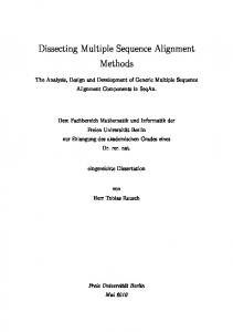
BLOSUM62 is standard for ungapped matching, and BLOSUM50 could be perhaps better for alignment with gaps. 2.3. Matrices Specificity Everybody would use the same matrix from a long time if a given one was a panacea. After testing 134 matrices to align a set of 78 family of known structures, results indicated that, each of them may be the most adapted to a given situation, but the best one is not predictable a priori [23]. We related by a factor analysis the score obtained by each matrix and the type of micro-environments coded in terms of secondary structure and solvent accessibility (exposed/buried). A clear gradient of specificity has been revealed, the PAM family being more efficient for exposed helices and BLOSUM family for the buried strands, generalist matrices being intermediary [24]. User is therefore concerned by the choice of the matrix, even if he is predisposed to keep the default matrix in case of divergence between results obtained with different matrices (see Fig. 1), validation by other criteria should be stressed. 3. PAIRWISE ALIGNMENT The pairwise alignment method can be divided into two categories [25], reflecting different perspectives. The first category considers the similarity across the full extent of the sequences, and will perform a "global alignment" [26,27]; the second focuses only on the regions where the similarity is present in some regions of the sequences, and will provide a "local alignment" [28,29]. These two types of alignments approaches will give different information. For example, the global alignments are interesting for evolutionary comparisons and local alignment are more useful for structural predictions, or comparison of sequences that share similarity only in a part of the sequence. Pairwise alignment generates high number of false positive but remains an essential and powerful tool for database searching mainly. Moreover, all methods that carry out comparison of sequences against a database, are essentially extensions of the concept of pairwise alignment algorithms. 3.1. The Dynamic Programming Algorithms One of the basic principle for finding optimal alignment for a pair of sequences is called the dynamic programming [30]. Dynamic programming algorithms are central in the field of computational sequence analysis. This kind of algorithm performs an alignment in two main steps [30]. In the first one, each amino acid of the first sequence is compared with each amino acid of the second sequence. All comparison results are marked and stored in a n x m matrix (sometimes called dot plot matrix), n and m being the size (in amino acids) of the two sequences. An algorithm will then search paths through the n x m matrix to find the optimal scoring alignment, each path being characterized with a score. If there are several possible paths, the choice of one path will depend mainly on the choice of several parameters such as the scoring matrices and the gap penalties.
Review of Common Sequence Alignment Methods
Current Genomics, 2003, Vol. 4, No. 2 133
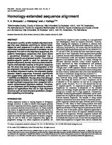
Fig. (1). Factor loadings for the first two factors of a principal component analysis performed on the following matrix: 48,121 lines represent segments defined from a set of 78 sequences of known structure (82) and 140 columns represent the micro-environment of each segment (helix, strand, loop, and 3 levels of exposition to solvent), and the alignment score obtained for 134 matrices. A zoom on the right details the score matrix classification obtained. .Matrices are grouped in families, and results show that PAM is more efficient to align exposed helices and BLOSUM to align buried beta-sheets. Generalist matrices show intermediate performances (79). As show this 2D scatterplot, well known matrix families were re-formed according to our criteria, and we point out that other families were more efficient in some specificity zones and less in others.
3.2. The Needleman and Wunsch Algorithm To obtain the optimal global alignment between two sequences allowing gaps, one can use a dynamic programming algorithm as the Needleman and Wunsch algorithm[30]. This algorithm is the most primary used to compute a global alignment between two sequences [30]. It is a matter of simple application of the strategy of the "best-path" using the concept of the dotplot like starting point. The results will then be interpreted computationally [30]. In this approach, the idea is to build up an optimal alignment using previous solutions used for optimal alignments of smaller subsequences. The greatest number of possible matches is defined between two sequences constructing a matrix M indexed by i and j, one proceed then to fill the matrix from top left to bottom right. At each step, the movement from one cell of the matrix towards another one is either a diagonal (two residues superposed in the final alignment) or a vertical or horizontal move, that correspond to an indel (insertion/deletion). Needleman and Wunsch proposed a path offering a maximum of matches, but the more efficient version was introduced by Gotoh in 1982 [31]. 3.3. The Smith-Waterman Algorithm When it is suspected that two protein sequences can share a common domain, we must look for the best alignment just between subsequences of these proteins [25]. The highest
scoring alignment of subsequences is the best local alignment. It is also usually the most sensitive way to detect a similarity between two very divergent sequences. In fact, only a part of the sequence has been under strong enough selection to preserve detectable similarity. The rest of the sequence will have accumulated so much noise through mutations that it is no longer possible to align [32]. The algorithm used to find optimal local alignments is a simple modification of the Needleman and Wunsch algorithm described in the previous section [32]. There are two main differences: First, in each cell in the matrix, one more possibility is added allowing M(i, j) to take the value 0 if all other options have value less than 0. When the score drops to 0, extension of path is terminated and a new one can start up. The second main change is that when an alignment end anywhere in the matrix, we are looking for the highest value of M(i,j) of the matrix, and restart the back-tracking from there. There can be many individual paths bounded by regions poorly matching. From these paths, those with the highest score are reported as the optimal local alignment. 3.4. Gap Penalty Input : Parameters or Output Result ? Insertion or deletion of some residues, essentially in loops, involves that similar regions aligned are shifted by several positions (20 or 30 residues) in the sequences [25]. Additionally, a whole domain may be missing in one of the sequences, as alignment could be shifted by 200 or 300
134 Current Genomics, 2003, Vol. 4, No. 2
Lambert et al.
residues [25]. In alignment outputs, gaps are inserted to compensate these indels, and are in fact the expected result of alignment algorithms. Similar sequences of exactly the same length do not need gaps neither alignment. But gaps have no structural meaning and criteria to evaluate the gap cost are essentially empirical [7]. Higher the number of gaps, higher the similarity between the residues aligned and more dubious the structural meaning of the result [33].
technique is based on the comparison of different models. A second approach is based on a statistical approach [38] by calculating the chance of having a match score greater than the observed one. This way considers significance in several situations [39]. To determine if an alignment is statistically significant we can do a permutation test.
To limit the number of gaps, the alignment score is reduced by a factor that depends on the gap penalty parameter [7]. Although a number of strategies have been proposed for penalizing gaps, the most common formulation involves a fixed deduction for introducing a gap plus an additional deduction proportional to the length of the gap. This is governed by two main parameters [34]:
(b). Aligning the new permuted sequences.
The opening gap penalty (G) is a penalty for the initiation of the gap in a sequence. A larger opening gap penalty can result in more significant matches and will result in to give a good alignment without many gaps. The gap extension penalty (L) is applied for increasing an already existing gap by one residue. As well as in the opening gap penalty case, increasing an extension gap penalty may increase the significance of the match. For a gap of a given length, the total score reduction would be G + Ln where n is the length of the gap [34]. Unfortunately, the selection of gap parameters is highly empirical and many alignment algorithms depend on a gap weighting parameter, which determines the number and length of gaps by introducing a gap cost for initiating and extending gaps. So, the expected result becomes a governing input parameter; and there is little theory to support the choice of any particular set of values. This is exactly as if a statistical program was asking to the user what difference between means he wants before performing a t test. Of course, an alignment result hardly depends of these empirical parameters and therefore few programs evaluate the reliability of a given solution [7]. So, the user may just use the default parameters, or can perform several runs and choose the output ‘that looks better’, for lack of rational discriminating criteria. A careful discussion about “gap penalties” can be found in a review of Vingron & Waterman [7]. The main problem with progressive global alignments like ClustalW [35,36] is probably that it is possible to assign a different weight to gaps, each set-up leading to a different result. 4. PERFORMANCE EVALUATION 4.1. Statistical Measures of Alignment Significance Now that we know how to obtain an alignment, how can we estimate the significance of this alignment and its score? Is it important to determine whether its score is high enough? How to decide if it is a biologically meaningful alignment giving evidence for a homology, or simply the best alignment between several unrelated sequences ? There are several approaches to tackle this topic [37]. The Bayesian
(a). Rearranging residues by random in one or all sequences.
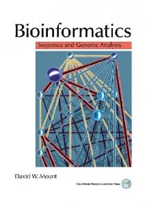
(c). Marking the scores obtained for this alignment. Repeating these steps a large number of times, generates a distribution of alignment scores that could be expected for the randomly rearranged sequences [38]. Then, we can look at the distribution of the maximum of N match scores of independent random sequences. If the probability of this maximum being greater than the observed best score is small, the observation can be considered as significant [40]. In accordance with Doolittle's rule for protein sequences, more than 25% identity will suggest homology, less than 15% would be doubtful [18] and for those cases between 1525% identity, a hard statistical argument would be required [39]. However, percentage of identity is defined after alignment and hardly depends on the method and its set-up [35]. When alignment is over-gapped, similarity is overestimated. Any standard program will produce a statistical index indicating the level of confidence that should be attached to an alignment. Our laboratory developed a program called MATCHBOX [41-43] that includes sequence alignment tools based on strict statistical thresholds of similarity between protein segments. MATCH-BOX is organized in two main programs: the first one, EXPLORE, being dedicated to pairwise similarity analysis, the second one, ALIGN (see 5.1.2), being dedicated to sequence alignment. EXPLORE scans the pairwise similarity between sequences, and tests their significance (see Fig. 2 and Table 1). Randomization of the sequence is used to check if the similarity between the sequences departs from the one expected by chance in unrelated sequences. If it is not the case, subsequent alignment is meaningless. Sequences are also plotted in a plane of factor analysis, in order to delineate relevant subgroup of sequences to align. To prepare homology modeling, sequence diverging from the couple target/ template should be removed. On the opposite, to detect conserved residues potentially implied in the protein function, too redundant sequences should be purged and the widest variety of related sequences conserved. EXPLORE is really an alternative way to consider significance in such situations. By way of example, we related in the bibliography below several of these situations which EXPLORE proved to be crucial in considering the significance [44-50]. 4.2. Confidence is a Critical Evaluation Criterion Test cases with proteins of known structure allow the definition of structurally conserved regions (SCR) to evaluate the performances of alignment algorithms [24]. To
Current Genomics, 2003, Vol. 4, No. 2 135
Review of Common Sequence Alignment Methods
Fig. (2). Cumulated frequency distribution of the distance between short segments before (diamond) and after (squares) random shuffling of the residues (Explore from Match-Box server). x-axis represents the class of distance between 9-residue segments computed from the current score matrix (by default: Blosum62). Frequency of matches is computed for each class and cumulated. Then the SUM+1 transformed in LOG10 (y-axis). The distance between the two curves, if any, represents the deviation of the similarity between sequences from randomness. When the curves are superimposed, the subsequent alignment is meaningless.
test prediction reliability of several multiple alignment methods, our laboratory defined an evaluation of algorithm performances based on two criteria: “power” (sensitivity) and “confidence” (selectivity), with confidence and power negatively correlated [9]. These criteria evaluate false negative as well as false positive in aligned positions. For a given ‘truth’ (based on structure alignment), let say 100 Table 1. The Reliability Score Shown in Figure 3 is Linearly Related to the Averaged OBSERVED Confidence in Structure Alignments. For Each Value of the Reliability Score and the Averaged Observed Confidence are Reported. Results are Expressed in % Confidence (Correctly Predicted/Total Aligned Positions) are Computed on 4900 Aligned Positions (23) Predicted Confidence Score
Observed Confidence Average
1
100
2
98
3
91
4
86
5
79
6
72
7
65
8
58
9
51
aligned positions in the structure, the power computes the part of the truth found in the solution (i.e. for 80 correct positions: power = 80%). Reciprocally, the confidence computes the part of the solution that is true (i.e. 80 correct positions, for 400 aligned positions in the structure: confidence = 20%). Power and confidence are logically inversely related: each effort to extend the part of the truth detected, i.e. thresholds softening, consequently increases the noise and lower the confidence. It is important to evaluate the performances of different methods not only in terms of power, but also in terms of confidence [9] (see Fig. 3). Molecular biologists do not seem adequately aware of the risk of error in alignments. Evaluations of alignment methods quite never take into account the confidence as a performance. This biased evaluation reinforces the tendency in getting algorithms more sensitive but less selective, and generates a high rate of false positive results. 4.3. Test Cases for the Evaluation of Alignment Performances To evaluate any alignment algorithms, we need a large number of accurate reference alignments [9]. So, this reference can be considered as true and used as test cases. Absolute comparisons between power and confidence rates can be achieved only for a given set of test cases and for a given definition of what has to be found (i.e. the truth). To evaluate power and confidence requires to define similar regions in a set of related sequences of known structure [9]. Only this region of reference allows the computing of underand over-estimations in sequence alignments. A test case
136 Current Genomics, 2003, Vol. 4, No. 2
Lambert et al.
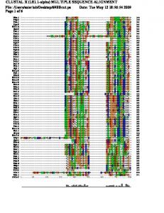
Fig. (3). Diagram representing the concept of power and confidence. Let us consider a jar containing light and dark cells, and results of independent essays to separate them placed in test-tubes, the goal being to keep only the dark cells. The power (x-axis) is the ratio between the number of light cells found in a test-tube and the total number of light cells in the jar (i.e.: n=10). The confidence (y-axis) is the ratio between the number of light cells found in a test-tube and the total number of cells in this test-tube. When similarity between sequences drops, alignment methods generate either high confidence with low power (up left) or high power with low confidence (bottom right).
requires several sequences sharing significant structural similarities despite of low sequence homology. To test multiple sequence alignment algorithms, at least 3 sequences must be included in the tests. Once the structural alignment is obtained and converted into sequence alignment, the simplest criterion is to consider as correctly aligned the whole non-gapped region [51], e.g. all the positions
occupied by a residue in all the sequences. This definition appears to be not restrictive enough, because the conserved regions are generally limited to the core of the protein, and alignment of residues of variable loops is not always relevant. A second possible criterion would be to consider as structurally conserved the secondary structures conserved in the whole set of sequences [24]. However, border effects and
Current Genomics, 2003, Vol. 4, No. 2 137
Review of Common Sequence Alignment Methods
the loose definition of coils limit these regions to the middle of helices and beta strands. Finally, the RMS distance computed between segments of protein considers not only the highly conserved helices and strands but also highly conserved loops and turns [52]. The RMS distance represents the residual mean square between the corres-ponding backbone atoms, generally C-Cα-N (sometimes limited to Cα, sometimes extended to oxygen), after optimal superimposition (minimized distance). However, the RMS obtained after a global superimposition of the structure is enable to delineate regions of relevant structural similarities between divergent but clearly homologous protein sequences as defined by Chothia & Lesk [53]. The 'best' truth is thus defined as short regions structurally superimposed according to a RMS threshold [54].
all sequences have been aligned. The iterative process compares the string with the smallest distance with any of the strings already in the multiple alignment [62].
To perform analysis of multiple alignment performance on a large set of test cases, Briffeuil et al. defined the truth using a RMS threshold of 2.5 Å. When working at the limit of the twilight zone with completely different approaches, he noted a ceiling at about 70% of power for several alignment methods [9].
Progressive alignment is a heuristic method: the most similar pairs of sequences are aligned first and it does not separate the process of scoring an alignment from the optimization algorithm.
5. MULTIPLE ALIGNMENT The main aim of multiple alignment is to show the underlying relationships between proteins, for a better comprehension of the evolution of these proteins [55]. Multiple alignments must usually be inferred from primary sequences alone [25]. Instead of examining a single protein, one can look at a family of related proteins to see how evolutionary pressures and biological economy have combined to produce new proteins having slightly different yet related functions. Manual multiple alignment is very tedious and automatic methods are today an important topic in computational biology [34]. A computational problem to provide a multiple alignment is the calculation time that will grow as Nm , where m is the number of sequences [56,57]. For this reason, computer-time accessible methods are widely fundamentally based on pairwise comparisons of sequences or segments [58-60] or on an alignment of sequence with a consensus [61]. Essentially, there are two main perspectives on the construction of alignments: the first approach is guided by the comparison of similar strings of amino acid residues [3]; the second results from comparison is at the level of secondary or tertiary structure, where alignment positions are determined on the basis of structural equivalence. Now, we review a set of different representative methods employed to carry out the multiple alignment. 5.1. Common Multiples Alignments Method 5.1.1. Progressive Methods The progressive method is probably the most commonly used approach in the field of multiple sequence alignment [62]. The main idea of this method is to construct a succession of pairwise alignments. First, two sequences are chosen and aligned by standard pairwise alignment and this alignment is fixed. Then, a third sequence is chosen and aligned to the first alignment. This process is iterated until
This strategy was introduced by several authors [58,6367]. A same fundamental approach is expressed by different original algorithms : - to choose the order to perform the alignment - to build up single growing alignment or whether subfamilies on a tree structure - to align and score sequences or alignments against existing alignments
The main advantage of the progressive strategy is that it is fast and efficient, and that it leads in many cases to a reasonable alignment. The main disadvantages of this approach are “the gap parameters” problem and of course that the subalignments are really frozen [58,68]. Moreover, early alignments are never thrown back: any mistakes made in intermediate pairwise alignments will be spread on the further steps, excepted if using an iterative refinement such as the Gotoh approach [69]. Clustal The Clustal is one widely used implementation of profile-based progressive multiple alignment. Based on the idea of progressive alignment, in much the same way as the Feng-Doolittle method except for its carefully tuned use of profile alignment methods. CLUSTALW [35] succeeded an earlier popular program, CLUSTALV [70]. The Clustal method profits from the fact that the similarity between sequences are probable to be evolutionarily related. From a set of sequences, CLUSTALW calculates a series of pairwise alignments scores (comparing each sequence one another), and convert them to two distances. From the distances by a neighbor-joining clustering algorithm, CLUSTALW builds a guide tree, which can be weighted to favor closely related sequences [68] and progressively align at nodes in order of decreasing similarity (using sequencesequence, sequence-profile, profile-profile). In addition to the customary methods of profile construction and alignment, several additional heuristics of CLUSTALW contribute to increase its performances: On one hand, the sequences can be weighted to compensate for biased representation in large sub-families. Its profile scoring function is a simply sum-of-pairs where as with Carrillo-Lipman [71], the sequences can be weighted to compensate for the defects of the sum-of-pairs. The scoring matrix is chosen on the basis of the similarity expected of the alignment; closely related sequences and distant sequences are aligned with different matrices (e.g. BLOSUM8O, BLOSUM50).
138 Current Genomics, 2003, Vol. 4, No. 2
On the second hand, to accommodate the divergences of sequences, it will undoubtedly be obligatory to insert gaps. In 1994, Thompson et al. described ClustalW using the positioning of residues to control the introduction of gaps into sequences that are more distant [72]. The specific position of gap-open penalties are multiplied by a modifier relating to the residues observed at this position. These penalties were calculated from gap frequencies observed in a large set of structural alignments. Generally, hydrophobic residues (which are more likely to be buried) give higher gap penalties than hydrophilic or flexible residues (which are more likely to be surface-accessible). This gap-open penalties are also decreased if the position is spanned by a segment of five or more consecutive hydrophilic amino acids Therefore ClustalW allows gap penalty so that gaps are preferentially opened in the less well conserved regions (typically surface loops). Now, the opening and the extension gap penalties are also both increased if there are no gaps in a column but nearby in the alignment so that to force all the gaps to occur in the same places in this alignment. This empirical approach, even sometimes operational, remains questionable and should be cross-referred by additional information such as experimental evidences. MultAlin MultAlin computes a multiple alignment from a set of related sequences. In 1988, Corpet described this method in "Multiple sequence alignment with hierarchical clustering", [73]. This method is based on a conventional dynamicprogramming method of pairwise alignment. A hierarchical clustering of the sequences is performed with a scoring matrix. The closest sequences are aligned creating sets of aligned sequences. After, this first alignment all sequences are aligned in one set. All the pairwise alignments included in the multiple alignment form another matrix that is used to produce a hierarchical clustering. If it is different from the first one, iteration of the process can be performed. The process continues until the score converge on a equivalent value, whereupon we have the final multiple sequence alignment. PileUp The PileUp method creates multiple sequence alignment using a similar simplification of the progressive alignment method of Feng and Doolittle [59]. The method also begins with the pairwise alignment of the two most similar sequences, and then performs a cluster hierarchy of the aligned sequences. Before alignment, a tree or a simple ordering represent the clustering relationship. The final alignment is achieved by several pairwise alignments including increasingly dissimilar sequences and clusters, until all sequences have been included in the final pairwise alignment. PileUp can plot the calculated dendrogram so that you can see the order of the pairwise alignments that created the final alignment. Multiple Alignment Program (MAP) MAP is another widely used multiple global alignment program. The fundamental algorithm of MAP uses an iterative pairwise approach to align two sequences. MAP
Lambert et al.
computes a best overlapping alignment between two sequences without penalizing gaps. Moreover, long internal gaps in short sequences are not strongly penalized. Thus MAP is good to produce an alignment where there are long terminal or internal gaps in some sequences. The MAP program is designed in a space-efficient manner; so long sequences can be aligned [74]. Pattern-Induced Multi-sequence Alignment (PIMA) PIMA performs a multiple alignment of a set of (presumably related) sequences using an extension of our covering pattern construction algorithm [75,76]. All pairwise comparisons between sequences in the set are performed and the resulting scores clustered into one or more families using two different linkage rules: “maximal linkage” [75] and “sequential branching” [76]. All pairwise scores are sorted high-to-low, the first sequence from the highest scoring pair is chosen as the "reference sequence", and the sequences clustered based strictly on the order of similarity to the reference sequence. Each cluster is then multiply aligned using a pattern-based alignment algorithm. Patterns are constructed using one of two extended amino acid alphabets. If secondary structure sequences are provided for one or more of the primary sequences (one of which must be designated as a "reference sequence") then the sequences are clustered using the sequentially branching rule and the set multiply aligned using a secondary structure dependent gap penalty algorithm. 5.1.2. Local Alignment There are cases where several sequences share a similar region but are otherwise completely different [42]. For example, the amino acids in the active site of an enzyme or transcription factor binding sites in a DNA sequence. To handle these cases, local multiple alignment algorithms have been developed [34]. Usually they only look for ungapped alignments, avoiding the problem to choose the optimal gap penalty. Indeed, the local alignment maximizes similarity of aligned fragments [41] and most local alignment methods do not allow gaps. The local similarities are measured between the partial sequences and the alignment is generated in which gaps are results not an input parameter. Match-Box At the beginning of the nineties, Depiereux and Feytmans developed a general protein sequence alignment methodology called Match-Box for detecting a priori unknown common structural and functional regions using two main programs, EXPLORE (see 4.1) and ALIGN [41,42,77]. Align is an original algorithm for simultaneous alignment using a fundamentally new way to match similar regions. The alignment is performed on all the sequences simultaneously, and the algorithm detects those regions that form a set of similar profiles and regardless of gap weighting. Complete matches are formed by segments more similar than expected by random, according to a given probability limit. An automatic screening delineates all the similar regions (boxes) that may be defined for a given maximal shift between the sequences. Align converges to the optimal solution with respect to objective statistical criteria,
Current Genomics, 2003, Vol. 4, No. 2 139
Review of Common Sequence Alignment Methods
building the alignment from boxes that have a very low probability to be observed by chance. Match-Box does not provide any alignment when sequences are unrelated. Many other methods align sequences from the first to the last residue, but Align clearly delineates the regions of the sequences that are aligned and the ones that are not. The reliable conserved regions outlined by Match-Box are particularly relevant for homology modeling of protein structures, prediction of essential residues for site directed mutagenesis and oligonucleotides design for cloning homologous genes by polymerase chain reaction. The MatchBox software differs from other classical alignment methods that provide a nearly optimal solution [9] by provided a score of confidence that is computed for each aligned position (see Fig. 4). This score has been shown to be linearly related to the confidence observed when aligning regions of test proteins superimposed according to the RMS criterion described above [9]. Dialign DIALIGN is a method for multiple alignment developed by Morgenstern et al. [78,79]. Its algorithm constructs pairwise and multiple alignments by comparing whole segments of the sequences instead of a traditional comparison of each residue. Pairwise as well as multiple alignments are constructed from gap-free pairs of equal length segments. These segment pairs are called 'diagonals'. Therefore DIALIGN does not use any gap penalty, thus avoiding this critical parameter. Once a diagonal is included into the alignment, it is fixed and cannot be removed at a later stage of the algorithm. Diagonals are not sorted according to their weights, but rather according to so-called overlap weights where motifs occurring in more than two sequences are preferred to motifs occurring in only two sequences [78]. This approach is especially efficient and
suited to detect a local homology and works reasonably efficiently in terms of computing time and memory [79]. PROBE Probe is a program to create and refine iteratively a multiple sequence alignment. Probe carries out a transitive search while determining which sequences are interrelated. For example, if a pairwise alignment show that sequences A and B are related, and a second alignment show that sequence B and C are related, then sequences A and C must be related even if a pairwise alignment between A and C failed to show directly the relationship. And thus, Probe performs a large number of BLAST [28]. During the assembly of this collection of related sequences, a series of alignments and realignments are carried out until the alignment cannot be improved anymore. Then, another stage of search in data base starts to find related sequences that were missed at the time of the first pass. PROBE carries out these stages until convergence of the results. It is a critical stage if a false positive contaminates the previous search. In general, PROBE can erase the putative false positives from the data during the subsequent iterations by a process called « jackknife » [80]. This provides a reliable measure of statistical significance (E-value). PROBE is currently employed to build a comprehensive data base database of protein alignment. Nevertheless, PROBE uses a heuristic method and it will not find exactly the same one alignment with various random seeds [81]. 5.2. Other Multiples Alignments Approaches, Using Hidden Markov Models, Genetic Algorithm and Bayesian Statistics The majority of automatic multiple alignments are now carried out using the “progressive” approach or variations on
Fig. (4). Alignment between lysozyme and alpha-lactalbumin discussed by McKenzie and Whites (93) and here aligned by MatchBox. Below each aligned position a score from 1 to 9 estimates the statistical significance of the alignment at this position. Lower the score is, higher is the reliability of the alignment. A score of 5 corresponds to a level of similarity of equal occurrence in related and unrelated sequences.
140 Current Genomics, 2003, Vol. 4, No. 2
it. There are some main alternatives to progressive alignment. These approaches have the advantage that their alignment is really (or closely) the best by some criterion. That is why many bioinformatics groups have adopted alternatives to progressive alignment such as Hidden Markov models (HMMs), Genetic Algorithms (Gas) or Bayesian statistic to resolve the multiple sequence alignment problems. The first category is a format of probabilistic form of statistical models of protein structure consensus called profiles [82]. One of the best introduction to the subject was described by Rabiner in 1989 [83]. The second category consists in a optimization methods to mimic the biological evolution. The Bayesian Statistic is a kind of approach that allows to bypass the substantial problem of parameter selection (scoring matrix and gap penalty). One of these main approaches uses hidden Markov models which are stochastic models composed of a large number of interconnected states, with for each state an observable output symbol [84] (see Fig. 5). Symbol emission probabilities are the probabilities of emitting each possible symbol from a state. This state sequence is "hidden" and only the symbol sequence it is emitting is observable [83]. State transition probabilities are the probabilities of moving from the current state to a new state using stochastic distribution determined by the state of the hidden Markov chain. HMM can simultaneously find an alignment and a probability model of substitutions, insertions and deletions, which is most self-consistent. The most probable path to align a sequence to a profile HMM is found by the Viterbi algorithm. And to build a multiple alignment requires the calculation for each individual sequence a Viterbi alignment [85]. Residues aligned to the same profile HMM match state are aligned in columns. At the present time, many multiple alignment methods are using hidden Markov models in their approach. For example, meta-MEME [86], HMMER [87], or Gibbs [88].
Lambert et al.
More basic introductions to HMMs include good reviews [84,89,90]. Another approach that we have not yet discussed here is algorithms using a stochastic optimization methods such as simulated annealing. Gibbs sampling algorithm described in 1993 by Lawrence et al. [88] is a short ungapped model which is essentially a profile HMM with no insert or delete states (very successfully applied to find the best local multiple alignment block with no gaps) [86,91] or genetic algorithms (GAs). Genetic Algorithms were described in 1987 by Goldberg [92] and then used in the context of multiple alignment because they are able to find an optimal multiple alignment in reasonable time using a population of potential possibilities which evolve by natural selection [92]. In the beginning, generation zero alignment is randomly created from the sequences to align. By several types of natural selection (called operator), a next generation is derived from the generation zero. Thus to create this generation, an operator is selected and could be a crossover (mixing the contents of the two parental sequences), gap insertion, block shuffling, rearrangement or a mutation. The method involves a population of alignments in quasi the same way of evolutionary and gradually increases the suitability of the population. This approach can be used for the multiple alignment problem. For example, SAGA uses an automatic strategy to control 22 different dynamically optimized operators for combining alignments [93]. Unfortunately, the number of possible alignments that must be scored in order to choose the best one becomes astronomical for more than four or five sequences of reasonable length [93]. Another approach to parameter estimation is to choose the mean of posterior distribution as the estimate, rather than the maximum value. This approach is part of a field of statistic called Bayesian [94]. Bayesian approach seeks to extract scene information to obtain an estimate [94]. In the
Fig. (5). Outline of a standard linear HMM where each node has a match state (square), insert state (diamond) and delete state (circle). Each sequence uses a series of these states to traverse the model from start to end.
Review of Common Sequence Alignment Methods
multiple sequence alignment domain, Bayesian inference algorithm which returns the posterior distribution of all alignments considering all range of gapping and scoring matrices selected, weighing each in proportion to its probability based on the data [95]. A problem with the Bayesian approach is computational complexity [96]. MSA The MSA program uses a clever algorithm for reducing the volume of the multidimensional dynamic programming matrix. The Carrillo & Lipman algorithm [71] was implemented in MSA [97]. Carrillo & Lipman assume a “sum of pairs” scoring system for residues and gaps [71]. The score of a multiple alignment is the sum of the scores of all pairwise alignments defined by the multiple alignment. A first bound is produced during this stage. Weights are usually applied to this value to produce the lower bound used by the program. Next a heuristic alignment is produced for the sequences. This heuristic alignment is produced by a procedure similar to progressive pairwise approach outlined above. Generally speaking, MSA will produce better alignments than most multiple sequence alignment programs such as Clustal [72] or PileUp. The disadvantage of MSA is that it requires an enormous amount of both computer time and memory (particularly for distantly related sequences) and directly correlated to the sequence lengths and the number of sequences [85]. All of these problems approached the limits of the problems that can be solved optimally by the MSA program. 6. PERSPECTIVES AND CONCLUSIONS Several papers have systematically tested the accuracy of different multiple alignment methods against structurally or manually generated alignments [9,69,98]. Another benchmark for the alignment methods was developed by Julie D. Thompson to evaluate several local and global multiple alignment programs [51]. The results of this study suggest that the reference alignments used as test cases affects the performance of alignments programs and not all of the alignment methods react in the same manner to the different problems presented in those test cases [51]. Our conclusions are confirmed by the work of Julie Thompson that should allow users select the most suitable technique according to their requirements in terms of selectivity and sensitivity and depending on the set of sequences to be aligned. Each aligned set of sequences consists of technique according to their requirements in terms of selectivity and sensitivity, depending on the set of sequences to be aligned. Our laboratory regularly tests prediction reliability of several multiple alignment local and global methods in terms of power and confidence. Our best set of tests is composed of manually refined structural alignments of 20 families of related proteins with low levels of identity [9]. Tests confirm that any powerful method remains reliable when the rate of identity decreases. More interestingly, results clearly show that for only some methods power and confidence decrease linearly with the rate of identity, while others emphasize reliability at the cost of lowered power.
Current Genomics, 2003, Vol. 4, No. 2 141
6.1. Additional Information Several algorithms have been designed to predict protein secondary structure [25]. The algorithms are based on different approaches and the programs achieve different accuracies (information is coming from a single residue, of a single sequence; Local interactions are taken into account; Information coming from homologous sequences is incorporated). PHD [99], one of the most popular software for protein secondary structure prediction is composed of several cascading neural networks previously trained on proteins of known structures [100]. PHD may generate its own alignment with the submitted sequence [101,102]. Direct comparison of secondary structure prediction with classical alignment often allows to delineate more accurately structurally conserved regions. Some experiences have shown that the best way to improve alignment is to add information [24]: advanced alignment researches strive for incorporating secondary structure predictions in sequence alignment algorithms [103] or even solvent accessibility predictions [104]. Increasing the number of related sequences included in the alignment may either improve or decrease the quality of the predictions substantially [9]. For some methods, the gain in power or in confidence is quite systematic; for others, the effect of the addition of homologous sequences is highly unpredictable. Also, extracting the consensus between several methods increases significantly the overall confidence of the predictions [9,105]. 6.2. Limits of Interpretation and Clues to Operate Precautions in handling different methods and time devoted to bioinformatics study hardly depend on the goal of the prediction [25]. A first guess of the possible function of an unknown sequence is obtained by running a simple BLAST [28]. To get a topological model requires a reliable prediction of secondary structure [105]. To locate residue potentially implied in the function of a given protein family requires robust multiple alignment. To build a 3-D model by homology below 30% of identity requests a very careful pairwise alignment [106]. More the bench work based on the rational design carried out in silico is consequent, more is the user concerned by the risk of false positive result. Is it really sensible to content oneself with one hour handling different tools on the Internet and selecting the result “that looks better” when site directed mutagenesis engaged to test the hypotheses takes one year? Hereafter we sum up some clues resulting from several unfortunate experience of hurried data miners: - The program will produce some statistical value indicating the level of confidence that should be attached to an alignment. For example, in pairwise comparisons for database searching where the statistics quoted are probability (p) or expected frequency (E) values. However, data mining
142 Current Genomics, 2003, Vol. 4, No. 2
Lambert et al.
in large databases generates oversampling, devaluating the statistical inference.
similarity is hard to interpret when similarity is not defined, as it is often the case.
The 'p-value' relates the score returned for an alignment to the likelihood of its occurrence by chance only. For a given event, i.e. the occurrence of "conserved" sequence motif, of probability about 0.0001, an extensive research on about 10,000,000 of segments of length 10 would generate about 1000 false positive hits!
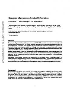
- Any prediction method offers simultaneously a low rate of false negative and positive result [9]. Performances of alignment methods (see Fig. 6), averaged on a range of similarities between sequences, reach up to 80% of power and a little less than 70% of confidence for ClustalW [9,25], or 65% power and 85% of confidence for Match-Box [9,43], which remains still today the most trustful of the multiple alignment methods tested by us. When the percentage of identity falls below 20%, confidence drops to 30% (50% of confidence means that one aligned position over two is unduly aligned) [9]. In a recent test on beta strand prediction of porins [105] performances of different methods of secondary structure prediction [99,105] vary from 52% to 94% for confidence and from 20% to 80% for power. For a given method, the range is comparable for different proteins of the test set.
In BLAST [28] the Expect value (E-value) describes the number of hits one can 'expect' to see by chance (in other words noise) when searching a database of a particular size. - Moreover, gap insertion will considerably raise the number of possibilities and consequently the risk of false positive results [51]. Number of identities between unrelated sequences may be raised up to 60% by allowing intensive gap insertion. “Swiss cheese” alignments of motives, even impressive according to identical aligned residue, suffer of a quite low predictive significance. - Percentage of identity is a very widespread criteria to characterize ranges of protein similarity and consequently of methods reliability. However, few users are aware of the fact that this statistic is computed after alignment, and hence hardly depends on the method and set-up used. Percentage of
- Even though programs such as Probe carries out a transitive search while determining which sequences are interrelated, similarity is not mathematically a transitive operator. By chaining effect, a similarity deduced from another similarity might be not relevant at all. A set of sequences often includes outsiders that interfere with the analysis, in particular for local alignment methods. Also, annotations
Fig. (6). Recent test of alignment methods performances. A given 'truth' (4900 aligned positions) is defined from local RMS (see text) computed on 20 families of structures of low sequence similarity. The power (x-axis) represents the part of the truth (%) aligned by the program and the confidence, (y-axis) the part of the alignment that is true. Seven methods are tested: prrp [64], ClustalW [33], Dialign [44,45], Multalin [38], saga [58], Match-Box [14,15], Map [96]. Match-Box is represented by two points, according to the level of confidence taken into account: all aligned positions (MB2) or positions of score ≤ 5 (MB1). Results show that methods peak up at an average of about 70% confidence. The only way to raise confidence - at lower power price- is to limit the reading to most reliable prediction (MB1).
Current Genomics, 2003, Vol. 4, No. 2 143
Review of Common Sequence Alignment Methods
servers: clues to enhance reliability of predictions, Bioinformatics 1998, 14 : 357-366.
found in database are often roughly deduced from automatic similarities and non-interpretable. - Sequence similarity provides no evidence of functional similarity [106]. For example, proteins between 10 and 20% of identity share, in average, structural similarity (80%), similar enzymatic function (50%), similar binding site (35%) [106]. - Running different methods and building consensus considerably raises the reliability of results [9,109]. A confidence score may be deduced from the number of methods leading to the same prediction. Inversely, clashing results occur in unpredictable situations. - Reliable pairwise alignments are often tricky to obtain. They should be extracted from multiple alignment, or from consensus of several multiple alignment methods [109].
[10]
Dayhoff, M.O., Schwartz, R.M. and Orcutt, B.C. A model of evolutionary change in proteins, Atlas of protein sequence and structure 1978, 5: 345-352.
[11]
Henikoff, S. and Henikoff, J.G. Amino acid substitution matrices from protein blocks, Proc. Natl. Acad. Sci. USA 1992, 89 : 10915-10919.
[12]
Overington, J., Donnelly, D., Johnon, M.S., Sali, A. and Blundell, TL. Environment-specific amino acid substitution tables: tertiary templates and prediction of protein folds, Protein Sci. 1992, 1: 516-526.
[13]
Luthy, R., McLachlan, A.D. and Eisenberg, D. Secondary structure-based profiles: use of structure-conserving scoring tables in searching protein sequence databases for structural similarities, Proteins 1991, 10 : 229-239.
[14]
Johnson, M.S. and Overington, J.P. A structural basis for sequence comparisons. An evaluation of scoring methodologies, J. Mol. Biol. 1993, 233: 716-738.
[15]
Loytynoja, A. and Milinkovitch, M.C. SOAP, cleaning multiple alignments from unstable blocks, Bioinformatics 2001, 17 : 573-574.
ACKNOWLEDGEMENT We thank N. Noël and B. Damien for helpful contribution and Guy Baudoux for fruitful discussions. Christophe Lambert holds a specialized grant from the 'Fonds pour la Formation à la Recherche dans l'Industrie et dans l'Agriculture' (F.R.I.A.).
SOAP is a stand-alone program to test the stability of a multiple alignment of molecular sequences by running ClustalW using a range of different parameters (gap penalties). SOAP identifies the 'unstable-henceunreliable' aligned columns by comparing a chosen set of alignments against a user-defined reference alignment.
REFERENCES [1]
Holm, L. and Sander, C. Searching protein structure databases has come of age, Proteins 1994, 19 : 165-173.
[2]
Attwood, T.K., Eliopoulos, E.E., Findlay, J.B. Multiple sequence alignment of protein families showing low sequence homology: a methodological approach using database pattern-matching discriminators for G-proteinlinked receptors, Genes 1991, 98 : 153-159.
[3]
[4]
[5]
[16]
Dayhoff, M.O., Barker, W.C. and Hunt, L.T. Establishing homologies in protein sequences, Methods Enzymol 1983, 91 : 524-545.
[17]
Doolittle, R.F. Of URFs and ORFs : a primer on how to analyze derived amino acid sequences, University Science Books, Mill Valley, CA, USA 1986.
Henneke, C.K. A multiple sequence alignment algorithm for homologous proteins using secondary structure information and optionally keying alignments to functionally important sites, Comput. Appl. Biosci. 1989, 5: 141-150.
[18]
Rost, B. Twilight zone of protein sequence alignments, Protein Eng. 1999, 12 : 85-94.
[19]
Vingron, M. and Argos, P. Determination of reliable regions in protein sequence alignments, Protein Eng. 1990, 3: 565-569.
Gonnet, G.H., Cohen, M.A. and Benner, S.A. Exhaustive matching of the entire protein sequence database, Sciences 1992, 256: 1443-1445.
[20]
Stormo, G.D. and Hartzell, G.W. III., Identifying protein binding sites from unaligned DNA fragments, Proc. Natl. Acad. Sci. 1989, 86 : 1183-1187.
Henikoff, S. and Henikoff, J.G. Performance evaluation of amino acid substitution matrices, Proteins 1993, 17 : 4961.
[21]
Henikoff, S. and Henikoff, J.G. Protein family classification based on searching a database of blocks, Genomics 1994, 19 : 97-107.
[22]
Pearson, W.R. Effective protein sequence comparison, Methods Enzymol. 1996, 266: 227-258.
[23]
Van, Campenhout, J-M., Lambert, C. and Depiereux, E. Development and testing of an Internet software for protein sequence alignment, Arch. Intern. Physiol. Biochem. Biophys. 1999, 107: B23.
[24]
Van, Campenhout, J-M., Lambert, C., De Bolle, X. and Depiereux, E. Exploiting the potentially informative prediction from protein sequences to improve sensitivity and selectivity of multiple sequence
[6]
Tramontano, A. Homology, modeling with low sequence identity, Methods 1998, 14 : 293-300.
[7]
Vingron, M. and Waterman, M.S. Sequence alignment and penalty choice : review of concepts, case studies and implications, J. Mol .Biol. 1994, 235: 1-2.
[8]
Bordo, D. and Argos, P. Suggestions for ‘safe’ Residue Substitutions in Site-Direct Mutagenesis, J. Mol. Biol. 1991, 217: 721-729.
[9]
Briffeuil, P., Baudoux, G., Lambert, C., De Bolle, X., Vinals, C., Feytmans, E. and Depiereux, E. Comparative analysis of seven multiple protein sequence alignment
144 Current Genomics, 2003, Vol. 4, No. 2
Lambert et al.
structurally conserved regions Engineering 1991, 4: 603-613.
alignment, Arch. Intern. Physiol. Biochem. Biophys. 1999, 110: B19. [25]
Attwood, T.K. and Parry-Smith, D.J. Introduction to bioinformatics, Addison Wesley Longman Limited, England 1999, 1-218.
[26]
Pearson, W.R. and Lipman, D.J. Improved Tools for Biological Sequence Analysis, Proc. Natl. Acad. Sci. 1988, 85 : 2444-2448.
[27]
Pearson, W. R. Rapid and Sensitive Sequence Comparison with FASTP and FASTA, Methods Enzymol 1990, 183: 63-98.
[28]
Altschul, S.F., Gish, W. Basic Local Alignment Search Tool, J. Mol. Biol. 1990, 215: 403-410.
[29]
Altschul, S.F. and Herickson, B.W. Locally optimal subalignments using nonlinear similarity functions, Bull. Math. Biol. 1986, 48 : 633-660.
[30]
Needleman, S.B. and Wunsch, C.D. A general method applicable to the search for similarities in the amino acid sequence of two proteins, J. Mol. Biol. 1970, 48 : 443453.
[31]
Gotoh, O. An improved algorithm for matching biological sequences, J. Mol. Biol. 1982, 162: 705-708.
[32]
Smith, T.F. and Waterman, M.S. Comparative biosequence metrics, J. Mol. Evol. 1981, 18 : 38-46.
[33]
Zhu, Z.Y., Sali, A. and Blundell, T.L. A variable gap penalty function and feature weights for protein 3-D structure comparisons, Protein Eng. 1992, 5: 43-51.
[34]
Baxevanis, A.D. and Ouellette, F.B.F. Bioinformatics a practical guide to the analysis of genes and proteins, Library of Congress Cataloging-in-publication Data 1998, 1-370.
[35]
Thompson, J.D., Higgins, D.G. and Gibson, T.J. CLUSTAL W: improving the sensitivity of progressive multiple sequence alignment through sequence weighting, position-specific gap penalties and weight matrix choice, Nucl. Acids Res. 1994, 22 : 4673-4680.
[36]
Higgins, D.G., Bleasby, A.J., Fuchs, R. CLUSTAL V: improved software for multiple sequence alignment, Comput. Appl. Biosci. 1992, 8: 189-91.
(SCR),
Protein
[42]
Depiereux, E. and Feytmans, E. Match-Box: a fundamentally new algorithm for simultaneous alignment of several protein sequences, Comput. Appl. Biosci. 1992, 8: 501-509.
[43]
Depiereux, E., Baudoux, G., Briffeuil, P., Reginster, I., De Bolle, X., Vinals, C., Feytmans, E. Match-Box server: a multiple sequence alignment tool placing emphasis on reliability, Comput. Appl. Biosci. 1997, 13 : 249-256.
[44]
de Fays, K., Tibor, A., Lambert, C., Vinals, C., Denoël, P., De Bolle, X., Wouters, J., Letesson, J.J. and Depiereux, E. Structure and function prediction of the Brucella abortus P39 protein by comparative modeling with marginal sequence similarities, Protein Eng. 1999, 12 : 217-223.
[45]
Bertrand, L., Vertommen, D., Freeman, P.M., Wouters, J., Depiereux, E., Di pietro, A., Hue, L. and Rider, M.H. Mutagenesis of the fructose 6-phosphate-binding site in the 2-kinase domain of 6-phosphofructo-2-kinase/ fructose-2,6-bisphosphatase, Eur. J. Biochem. 1998, 254: 490-496.
[46]
Bertrand, L., Vertommen, D., Depiereux, E., Hue, L., Rider, M.H. and Feytmans, E. Modeling the 2-kinase domain of 6-phosphofructo-2-kinase/fructose-2,6-bisphosphatase on adenylate kinase, Biochem. J. 1997, 321: 615-621.
[47]
De Bolle, X., Vinals, C., Prozzi, D., Paquet, J.Y., Leplae, R., Depiereux, E., Vandenhaute, J. and Feytmans, E. Identification of residues potentially involved in the interactions between subunits in yeast alcohol dehydrogenases, Eur. J. Biochem. 1995, 231: 214-219.
[48]
Vinals, C., De Bolle, X., Depiereux, E. and Feytmans, E. Knowledge-based modeling of the D-lactate dehydrogenase three-dimensional structure, Proteins 1995, 21 : 307-318.
[49]
Delforge, D., Depiereux, E., De Bolle, X., Feytmans, E. and Remacle, J. Similarities between alanine dehydrogenase and the N-terminal part of pyridine nucleotide transhydrogenase and their possible implication in the virulence mechanism of Mycobacterium tuberculosis, Biochem. Biophys. Res. Comm. 1993, 190: 1073-1079.
[50]
Vinals, C., Depiereux, E. and Feytmans, E. Prediction of structurally conserved regions of D-specific Hydroxy acid dehydrogenases by multiple alignment with formate dehydrogenase, Biochem. Biophys. Res. Comm. 1993, 192: 182-188.
[37]
Waterman, M. Estimating statistical significance of sequence alignments, Phil. Trans. R. Soc. Lond. 1994, 344: 383-390.
[38]
Karlin, S. and Altschul, S.F. Method for assessing the statistical significance of molecular sequence features by using general scoring schemes, Proc. Natl. Acad. Sci. USA 1990, 87 : 2264-2268.
[51]
Thompson, J.D., Plewniak, F. and Poch, O. BAliBASE: a benchmark alignment database for the evaluation of multiple alignment programs, Bioinformatics 1999, 15 : 87-8.
[39]
Karlin, S. and Altschul, S.F. Applications ans statistics for multiple high-scoring segments in molecular sequences, Proc. Natl. Acad. Sci. USA 1993, 90 : 58735877.
[52]
Greer, J. Comparative model-building of mammalian serine protease, J. Mol. Biol. 1981, 153: 1027-1042.
[53]
Chotia, C. and Lesk, A.M. The relation between the divergence of sequence and structure in proteins, EMBO Journal 1986, 5: 823-826.
[54]
Unger, R., Harel, D., Wherland, S. and Sussman, J.L. A 3D building blocks approach to analyzing and predicting structure of proteins, Proteins 1989, 5: 355-73.
[40]
Fitch, W.M. Random sequences, J. Mol. Biol. 1983, 163: 171-176.
[41]
Depiereux, E. and Feytmans, E. Simultaneous and multivariate alignment of protein sequences: correspondence between physiochemical profiles and
Current Genomics, 2003, Vol. 4, No. 2 145
Review of Common Sequence Alignment Methods
[55]
Sankoff, D. The early introduction of programming into computational Bioinformatics 2000, 16 : 41-47.
dynamic biology,
[56]
Gotoh, O. Significant Improvement in Accuracy of Multiple Protein Sequence Alignments by Iterative Refinement as Assessed by Reference to Structural Alignments, J. Mol. Biol. 1996, 264: 823-838.
[73]
Corpet, F. Multiple sequence alignment with hierarchical clustering, Nucl. Acids Res. 1988, 16 : 10881-10890.
[74]
Huang, X. On Global Sequence Alignment, Comput. Appl. Biosci. 1994, 10 : 227-235.
[75]
Smith, R.F., Anneau, T.M., Chandrasgaran, S. Finding sequence motifs in groups of functionally related proteins, Proc. Natl. Acad. Sci. 1990, 87 : 826-830.
[76]
Smith, R.F. and Smith, T.F. Pattern-induced multisequence alignment (PIMA) algorithm employing secondary structure-dependent gap penalties for use in comparative protein modelling, Protein Eng. 1992, 5: 35-41.
[77]
Depiereux, E. and Baudoux, G. Match-Box server: a multiple sequence alignment tool placing emphasis on reliability, Comput. Appl. Biosci. 1997, 13 : 249-256.
[78]
Morgenstern, B., Dres, A. and Werner, T. Multiple DNA and protein sequence alignment based on segment-tosegment comparison, Proc. Natl. Acad. Sci. 1996, 93 : 12098-12103.
[57]
Wareham, H.T. A simplified proof of the NP- and MAXSNP- hardness of multiple sequence tree alignment, J. Comput. Bio. 1995, 2: 509-514.
[58]
Barton, G.J. and Sternberg, M.J. A strategy for the rapid multiple alignment of protein sequences, J. Mol. Biol. 1987, 198: 327-337.
[59]
Feng, D.F. and Doolittle, R.F. Progressive alignment of amino acid sequences and construction of phylogenetics trees from them, Methods Enzymol 1996, 266: 368-382.
[60]
Subbiah, S. and Harrison, S.C. A method for multiple sequence alignment with gaps, Mol. Biol. 1989, 209: 539-548.
[61]
Gribskov, M., McLachlan, A.D. and Einsenberg, D. Profile analysis : detection of distantly related proteins, Proc. Natl. Acad. Sci. 1987, 84 : 4355-4358.
[79]
Morgenstern, B., Fresh, K., Dres, A., Werner, T. DIALIGN: Finding local similarities by multiple sequence alignment, Bioinformatics 1998, 14 : 290-294.
[62]
Sankoff, D. Minimal mutation trees of sequences, SIAM J. Appl. Math. 1975, 28 : 35-42.
[80]
[63]
Hogeweg, P. and Hesper, B. The alignment of sets of sequences and the construction of phyletic trees : an integrated method, J. Mol. Evol. 1984, 20 : 175-186.
Swofford, D.L., Olsen, G.J., Waddell, P.J. and Hillis, D.M. Phylogenetic inference. In molecular Systematics, Hillis, D.M., Moritz, C., Mable, B.K. Eds. (Sunderland, M.A.: Sinauer Associates) 1996, 407-514.
[81]
Waterman, M.S. and Perlwitz, M.D. Line geometries for sequence comparisons, Bulletin of Mathematical Biology 1984, 46 : 567-577.
Neuwald, A.F., Liu, J.S., Lipman, D.J. and Lawrence, C.E. Extracting protein alignment models from the sequence database, Nucl. Acids Res. 1997, 25 : 1665-1677.
[82]
Feng, D.F. and Doolittle, R.F. Progressive sequence alignment as a prerequisite to correct phylogenetic trees, J. Mol. Evol. 1987, 25 : 351-360.
Baldi, P., Hunkapiller, Y., Chauvin, T. and McClure, M.A. Hidden Markov Models of biological primary sequence information, Proc. Natl. Acad. Sci. 1994, 91 : 1059-1063.
[83]
Rabiner, L.R. A tutorial on Hidden Markov Models and selected applications in speech recognition, Proceedings of IEEE 1989, 77 : 257-286.
[84]
Krogh, A., Brown, M., Mian, I.S., Sjolander, K. and Haussler, D. Hidden Markov Models in computational biology : applications to protein modeling, J. Mol. Biol. 1994, 234: 1501-10531.
[85]
Durbin, R., Eddy, S., Krogh, A. and Mitchison, G. Biological sequence analysis : Probabilistic models of proteins and nucleic acids, Cambridge University Press 1998.
[86]
Bailey, T.L. and Elkan, C. The value of prior knowledge in discovering motifs with MEME, In Rawlings, C., Clark, D., Altman, R., Hunter, L., Lengauer, T. and Wodak, S. Proceedings of Third International Conference on Intelligent Systems for Molecular Biology 1995, 21-29 AAAI Press.
[87]
Eddy, S.R. Multiple alignment using Hidden Markov Models, In Rawlings, C., Clark, D., Altman R., Hunter, L., Lengauer, T. and Wodak, S. Proceedings of Third International Conference on Intelligent Systems for Molecular Biology 1995, 114-120 AAAI Press.
[88]
Lawrence, C.E., Altschul, S.F., Boguski, M.S., Liu, J.S., Neuwald, A.F. and Wotton, J.C. Detecting subtle
[64]
[65]
[66]
Taylor, W.R. Multiple sequence alignment by pairwise algorithm, Comput. Appl. Biosci. 1987, 3: 81-87.
[67]
Higgins, D.G. and Sharp, P.M. Fast and sensitive multiple sequence alignments on a microcomputer, Comput. Appl. Biosci. 1989, 8: 189-191.
[68]
Berger, M.P. and Munson, P.J. A novel randomized iterative strategy for aligning multiple protein sequences, Comput. Appl. Biosci. 1991, 7: 479-484.
[69]
Gotoh, O. Significant improvement in accuracy of multiple protein sequence alignments by iterative refinement as assessed by reference to structural alignments, J. Mol. Biol. 1996, 264: 823-838.
[70]
Saitou, N. and Nei, M. The neighbor-joining method : a new method for reconstructing phylogenetic trees, Molecular Biology and Evolution 1987, 4: 406-425.
[71]
Carillo, H. and Lipman, D. The multiple sequence alignment problem in biology, SIAM Journal of Applied Mathematics 1988, 48 : 1073-1082.
[72]
Thompson, J.D., Higgins, D.G. and Gibson, T.J. Improved sensitivity of profile searches through the use of sequence weights and gap excision., Comput. Appl. Biosci. 1994, 10 : 19-29.
146 Current Genomics, 2003, Vol. 4, No. 2
Lambert et al.
sequence signals : a Gibbs sampling strategy for multiple alignment, Science 1993, 262: 208-214. [89]
Gribskov, M. Profile analysis, Methods Mol. Biol. 1994, 25 : 247-266.
[90]
Krogh, A. and Mitchison, G. Maximum entropy weighting of aligned sequences of protein or DNA, In Rawlings, C., Clark, D., Altman, R., Hunter, L., Lengauer, T. and Wodak, S. Proceedings of Third International Conference on Intelligent Systems for Molecular Biology 1995, 215-221, AAAI Press.
[91]
Bailey, T.L. and Elkan, C. Fitting a mixture model by expectation maximization to discover motifs in biopolymers, In Altman, R., Brutlag, D., Karp, P., Latthrop, R. and Searls, D. eds., Proceedings of Second International Conference on Intelligent Systems for Molecular Biology 1994, 28-36, AAAI Press.
[92]
Goldberg, D. The genetic Algorithm, Artificial Life 1987, 154-187.
[93]
Notredame, C. and Higgins, D.G. SAGA: sequence alignment by genetic algorithm., Nucl. Acids Res. 1996, 24 : 1515-1524.
[94]
Box, G.E.P. and Tiao, G.C. Bayesian Inference Statistical Analysis, Wiley-Interscience 1992.
[95]
Zhu, J., Liu, J.S. Bayesian adaptive alignment and inference, Ismb 1997, 5: 358-68.
[96]
Zhu, J., Liu, J.S. Bayesian adaptive sequence alignment algorithms, Bioinformatics 1998, 14 : 25-39.
[97]
Lipman, D.J., Altschul, S.F. and Kececioglu, J.D. A tool for multiple sequence alignment, Proc. Natl. Acad. Sci. 1989, 86 : 4412-4415.
[98]
McClure, M.A., Vasi, T.K. and Fitch, W.M. Comparative analysis of multiple protein-sequence alignment methods, J. Mol. Evol. 1994, 11 : 571-592.
[99]
.
in
Rost, B. and Sander, C. Prediction of secondary structure at better than 70% accuracy, J. Mol. Biol. 1993, 232: 584599.
[100] Rost, B. and Casadio, R. Prediction of helical transmembrane segments at 95% accuracy, Protein Sci. 1995, 4: 521-533. [101] Rost, B. and Sander, C. PHD--an automatic mail server for protein secondary structure prediction, Comput. Appl. Biosci. 1994, 10 : 53-60. [102] Rost, B., Fariselli, P. and Casadio, R. Topology prediction for helical transmembrane proteins at 86% accuracy, Protein Sci. 1996, 7: 1704-1718. [103] Lambert, C., Noel, N., Van Campenhout, J-M., De Bolle, X. and Depiereux, E. Improving multiple sequence alignment using secondary structure prediction, Arch. Intern. Physiol Biochem. Biophys. 2000, 110: B11. [104] Van Campenhout, J-M., Lambert, C., De Bolle, X. and Depiereux, E. A new strategy algorithm to improve power and confidence of multiple sequence alignment by exploiting informative prediction programs, Protein Sci. 2000, 9: 76. [105] Paquet, J-Y., Vinals, C., Wouters, J., Letesson, J-J. and Depiereux, E. Evaluation of 3-state secondary structure prediction methods in porin topology prediction and application to Brucella abortus Omp2b porin, Journal of biomolecular structure & dynamics 2000, 17 : 4. [106] Devos, D. and Valencia, A. Practical limits of function prediction, Proteins 2000, 41 : 98-107. [107] Sauder, M.J., Arthur, J.W., Dunbrack, R.L. Jr. Large-Scale comparison of Protein Sequence alignment Algorithms With Structure Alignments, Proteins 2000, 40 : 6- 22. [108] Sali, A. and Blundell, T.L. Definition of general topological equivalence in protein structures. A procedure involving comparison of properties and relationships through simulated annealing and dynamic programming, Mol. Biol. 1990, 212: 403. [109] Bucka-Lassen, K., Caprani, O., Hein, J. Combining many multiple alignments in one improved alignment, Bioinformatics 1999, 15 : 122-130.