Review of modern logistic regression methods with ... - Semantic Scholar

Review of modern logistic regression methods with application to small and medium sample size problems Enes Makalic and Daniel F. Schmidt The University of Melbourne, Centre for MEGA Epidemiology, 723 Swanston Street, Carlton VIC 3053, Australia {emakalic,dschmidt}@unimelb.edu.au

Abstract. Logistic regression is one of the most widely applied machine learning tools in binary classification problems. Traditionally, inference of logistic models has focused on stepwise regression procedures which determine the predictor variables to be included in the model. Techniques that modify the log-likelihood by adding a continuous penalty function of the parameters have recently been used when inferring logistic models with a large number of predictor variables. This paper compares and contrasts three popular penalized logistic regression methods: ridge regression, the Least Absolute Shrinkage and Selection Operator (LASSO) and the elastic net. The methods are compared in terms of prediction accuracy using simulated data as well as real data sets. Keywords: Logistic regression; Variable Selection; LASSO; Elastic Net; Ridge regression

1

Introduction

Logistic regression is one of the most widely applied machine learning algorithms in binary classification problems. The popularity of logistic regression is due to the relatively low computational complexity of fitting the model parameters and the high interpretability of the logistic model. Fitting a logistic regression model is commonly done using the iteratively-reweighted least squares (IRLS) algorithm which is efficient provided the number of predictor variables is not too large. Most statistical software packages in use today implement some form of c has the logit() function. Unlike black-box algoIRLS; for example, STATA rithms, such as artificial neural networks, logistic regression models are highly interpretable and thus can be used in scenarios where interpretation of the model is as important as prediction accuracy. Formally, one observes p predictor variables (or covariates) x ∈ Rp and a binary target (or response) variable y ∈ {−1, +1} which states the class membership of the observed vector of predictors. The conditional probability that a vector of covariates x is assigned to a class y in logistic regression is p(y = ±1|x, β) =

1 1 + exp(−yx′ β)

(1)

2

Review of modern logistic regression methods

where β ∈ Rp are the regression coefficients. A positive regression coefficient for a predictor implies that the predictor is associated with an increased probability of the response (y = +1), while a negative coefficient reduces the response probability. A predictor with a regression coefficient of zero has no effect on the probability of the response and should ideally be excluded from the model. In order to make accurate predictions, one must estimate the parameter coefficients and select which of the p predictors, if any, are useful in explaining the response. In practice, one typically observes a set of independent observations D = {(x1 , y1 ), . . . , (xn , yn )} and proceeds by forming the log-likelihood l(β) = −

n X

log (1 + exp(−yi x′i β))

(2)

i=1

which is a function of the regression parameters β. A commonly used estimator of β is the the maximum likelihood estimator obtained by finding the parameters β that maximise the log-likelihood function. Traditionally, a stepwise regression procedure combined with the maximum likelihood method for parameter inference is used to determine significant predictors and their contribution to the probability of the target variable. The decision to include a new regressor in the model at each stage in the selection process is then based on the one set of data. This practice of data re-use, or data dredging, is known to be problematic and can often result in biased selection of significant predictors. More recently, techniques that modify the log-likelihood by adding a penalty function of the parameters have been used when inferring logistic models with a large number of predictor variables. This paper considers three popular penalized logistic regression algorithms: ridge regression [6], the Least Absolute Shrinkage and Selection Operator (LASSO) [11] and the elastic net [12]. Analysis of these methods in the literature has largely focused on the linear regression model in the asymptotic setting (that is, as the sample size or the number of predictors approaches infinity). In contrast, there has been relatively little research on the performance of penalized logistic regression methods, especially in small and medium sample size problems. This is somewhat surprising given the popularity of logistic regression in practice. This paper aims to address the aforementioned gap by comparing and contrasting three popular logistic regression algorithms in the small to medium sample size setting. Due to the mathematical complexity of the logistic model, all performance comparisons will be empirical and use both simulated data as well as real data sets.

2 2.1

Logistic regression algorithms Stepwise regression

Stepwise regression encompasses a range of procedures for automatic selection of significant predictors for linear or logistic regression models. Stepwise regression

Review of modern logistic regression methods

3

algorithms can be divided into two broad categories: (1) forward selection, and (2) backward elimination. In forward selection, the algorithm starts with all predictors excluded from the model and, at each step, includes a single predictor variable that is statistically important. For example, statisticians often include a predictor that results in the largest reduction of the log-likelihood at each stage in the selection process. The process is continued until all variables are included in the model or until some pre-determined threshold is met. In contrast, backward elimination begins with the full model that includes all p predictors and at each step removes a predictor from the model that does not result in a significant change to the log-likelihood. Like in forward selection, the elimination process continues until either all predictors are excluded or some performance threshold is met. It is also possible to use a hybrid strategy that considers inclusion and removal of regressors at each step. Due to the similarity of the various stepwise regression procedures, this paper considers only the forward selection algorithm. Given a model proposed by forward selection, it remains to infer the model parameters β. The most popular approach of parameter inference and the one considered in this paper is that of maximum likelihood. The maximum likelihood estimator is the estimator that maximises the likelihood or the log-likelihood (2). Formally, the maximum likelihood estimator of the logistic model parameters is ) ( n X ′ ˆ log (1 + exp(−yi x β) (3) βML = arg max − β

i

i=1

The maximum likelihood estimator must be obtained numerically. Due to the convexity of the log-likelihood, the estimator is unique unless the data is completely (linearly) separable. The main disadvantage of forward selection and stepwise regression in general is that the same data set is used for testing whether a predictor is included (or excluded) at each stage in the algorithm. Each test is therefore conditioned on the assumption that the previous inclusion (or exclusion) of predictors is ‘correct’. Statistical corrections for this multiple testing problem are possible, but are by no means trivial. Consequently, forward selection can result in a biased selection of pertinent predictors.

3

Penalized logistic regression

It is well known that the method of maximum likelihood often overestimates logistic regression parameters resulting in models that predict poorly. In order to tackle this problem a number of methods that shrink the parameters and perform automatic variable selection have been proposed. This paper examines the three most popular penalized logistic regression methods in use today: (1) ridge regression, (2) the Least Absolute Shrinkage and Selection Operator (LASSO) [11], and (3) the elastic net [12]. Note that forward selection may also be viewed as a type of penalized regression where the penalty function is the ℓ0 norm. A Bayesian implementation of penalized logistic regression is briefly considered in Section 4.

4

3.1

Review of modern logistic regression methods

Ridge regression

Ridge regression [6, 2] maximises the log-likelihood subject to a penalty on the size of the regression parameters. This results in continuous shrinking of the maximum likelihood parameter estimates which is known to improve prediction accuracy. Formally, the ridge regression estimator is ( ) p X 2 βˆRR = arg max l(β) − λ β (4) i

β

i=i

where the penalty parameter λ ≥ 0 determines the amount of shrinkage; for example, λ = 0 denotes no shrinkage, while λ → ∞ results in all parameters being shrunk to zero. Ridge regression can often result in models that predict well but cannot infer sparse models, a sparse model being one where majority of the coefficients are zero. Ridge regression either shrinks all parameters to zero or includes all predictors in the model. 3.2

Least absolute shrinkage and selection operator

Least absolute shrinkage and selection operator (LASSO) [11] employs a ℓ1 penalty on the regression parameters rather than the ℓ2 penalty of ridge regression. This results in a procedure that simultaneously performs parameter shrinkage and pertinent variable selection automatically. Formally, the LASSO estimator is ( ) p X βˆLA = arg max l(β) − λ |βi | (5) β

i=i

where λ ≥ 0 determines the amount of shrinkage. The main advantage of LASSO over ridge regression is that it can generate sparse models which are easier to interpret. However, the LASSO can exhibit undesirable behaviour in the presence of highly correlated predictors. For example, if there is a group of predictors which are highly correlated, the LASSO tends to randomly include one predictor from the group ignoring the other predictors. In addition, empirical observations [11] show that ridge regression dominates the LASSO in linear models when there are many correlated predictors. 3.3

Elastic net

Recently, Zou and Hastie have proposed a new penalized regression technique, the elastic net [12], to address the poor performance of LASSO given many correlated predictors. Like the LASSO, elastic net can produce sparse models as well as shrink parameter coefficients. However, if there is a group of highly correlated predictors, the elastic net includes all the predictors in the group thereby improving prediction performance. The elastic net penalty is a combination of the LASSO and ridge regression penalties, defined as ) ( p p X X β2 |βi | − λ2 (6) βˆEN = arg max l(β) − λ1 β

i

i=i

i=i

Review of modern logistic regression methods

5

where (λ1 , λ2 ) ≥ 0 are the penalty parameters. In contrast to ridge regression and the LASSO, elastic net requires inference of two extra penalty parameters which can be computationally demanding. Furthermore, it has been observed that the elastic net can overshrink the regression parameters in linear models. An empirical correction for this behaviour is available but only for the linear regression model.

4

Bayesian logistic regression

Penalized regression methods can be interpreted within the Bayesian statistics paradigm. Here, the log-likelihood penalty takes the form of a prior distribution over the parameter coefficients β. For example, ridge regression can be viewed as a Bayesian method where the prior for the parameters is a multivariate Gaussian distribution; the variance of the distribution being a function of the penalty parameter λ. Similarly, the LASSO penalty amounts to assuming a Laplace prior distribution over the parameter coefficients. Inference proceeds by forming a posterior distribution of the parameters conditioned on the data. Bayesian algorithms for penalized logistic regression have received relatively little attention, perhaps due to the mathematical complexity of the logistic model. Bayesian sampling approaches based on various approximations to the posterior distribution are examined in [9, 10]. An exact sampling scheme for the logistic distribution through data augmentation was introduced in [7]. Recently, an efficient scheme based on z-distributions is given by Gramacy and Polson [4]. We briefly examine how the Bayesian interpretation of the various penalized regression methods compares to the standard algorithms in Section 5.2.

5

Empirical comparison

Although a number of papers review penalized logistic regression [1, 5], relatively little work has been published on empirical performance of modern logistic regression methods in small to medium sample size applications. The methods chosen here represent the most popular approaches to penalized logistic regression in the literature. The all-subset selection algorithm was not tested because of the inherent instability (high variance) as well as prohibitive computational complexity of the method; for p regressors, all-subset selection requires fitting 2p logistic models! Various extensions of the ridge regression and LASSO, such as for example group LASSO, which have been developed for correlated predictors have also been omitted. A number of these algorithms require that the correlation groups are pre-defined before executing the method. This is generally not possible in practice. Lastly, the DANTZIG [8] selector was not included in the simulation experiments due to it’s high similarity to the LASSO. The selected logistic regression methods are now compared using both real c enviand simulated data. All simulation code was written in the MATLAB ronment and is available from the authors upon request. Special care was taken during implementation of numerical optimisation routines since both the LASSO

6

Review of modern logistic regression methods

and elastic net are not differentiable at βi = 0. Furthermore, standard NewtonRaphson optimisation requires costly matrix inversion and is only feasible when the number of predictors is relatively small. We have implemented a cyclic coordinate descent algorithm [3] which can be applied to a large number of predictors and gracefully handles minimisation of the LASSO and elastic net functions. 5.1

A simulation study

We have simulated data sets from four different scenarios originally examined in [12] and reproduced here for convenience. For each simulation, we independently generated a training set, a validation set and a test set. All regression parameters were estimated using only the training data. The validation data set was used to select the optimal penalty parameters, for the ridge, LASSO and elastic net algorithms, and the best model for the forward selection procedure. The optimal penalty parameters were computed using a grid search over a lattice recommended in [12]. The performance of the methods was computed using only the test data set. We have chosen the entropy loss function, rather than 0/1 loss, for this purpose. Unlike the 0/1 loss, the entropy loss is a convex, differentiable function that uses estimated probabilities to compute classification error and does not require specification of an arbitrary hard threshold. The entire procedure was repeated for 1000 iterations. The notation ·/ · /· is subsequently used to denote the sample size of the training, validation and test sets respectively. The four scenarios are: 1. Example 1: The number of samples was 20/20/200. The true regression coefficients were set to β = (3, 1·5, 0, 0, 2, 0, 0, 0)′ . The pairwise correlation between predictors i and j was corr(i, j) = 0.5|i−j| . 2. Example 2: Same as Example 1, except that βi = 0.85 for all i. 3. Example 3: The number of samples was 100/100/400 and corr(i, j) = 0.5 for all i and j. The regression coefficients (p = 40) were β = (0, . . . , 0, 2, . . . , 2, 0, . . . , 0, 2, . . . , 2)′ | {z } | {z } | {z } | {z } 10

10

10

10

4. Example 4: The number of samples was 50/50/400. The regression coefficients (p = 40) were β = (3, . . . , 3, 2, . . . , 2, 0, . . . , 0)′ | {z } | {z } | {z } 10

15

25

The predictors were generated from:

xi = Z1 + ǫi , Z1 ∼ N (0, 1), i = 1, . . . , 5 xi = Z2 + ǫi , Z2 ∼ N (0, 1), i = 6, . . . , 10 xi = Z3 + ǫi , Z3 ∼ N (0, 1), i = 11, . . . , 15 and xi ∼ N (0, 1) for i = 16, . . . , 40, where N (0, 1) represents the standard normal variable and ǫj ∼ N (0, 0·01) for j = 1, . . . , 15.

Review of modern logistic regression methods Method

Simulation Example 1

Stepwise Ridge LASSO Elastic net

7

0·6046 0·4215 0·4202 0·4158

(0·139) (0·028) (0·039) (0·033)

Example 2 0·7012 0·4249 0·4941 0·4381

(0·017) (0·023) (0·041) (0·028)

Example 3 0·0669 0·0534 0·0527 0·0527

(0·001) (0·001) (0·001) (0·001)

Example 4 0·5088 0·2477 0·2265 0·2280

(0·008) (0·002) (0·002) (0·002)

Table 1. Mean entropy loss for the four simulation examples based on 1000 test iterations; bootstrap estimates of standard errors given in parentheses

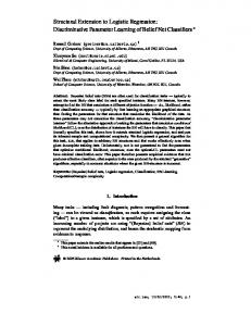
In all simulations, the targets y were generated uniformly with probability given by (1). Example 1 and Example 2 depict scenarios where the true model is sparse and dense respectively, while Example 3 and Example 4 simulate data with grouped predictor variables. Mean entropy loss for the four simulation scenarios is shown in Table 1. Stepwise regression had the largest mean entropy loss of all the methods tested in the four scenarios. In contrast, the three penalized regression methods performed relatively well, with the elastic net having a slight edge over ridge regression and the LASSO. LASSO performed poorly in Example 2 when compared to ridge regression and the elastic net. Ridge regression achieved the lowest entropy loss here which is not unexpected given that the predictors form a dense set. It is somewhat surprising that LASSO and ridge regression performed quite well on grouped predictor variables in Examples 3 and 4. Of the three penalized logistic regression methods, the authors recommend the elastic net as it achieves amongst the lowest entropy loss in all the scenarios tested. The elastic net is able to handle both sparse and dense predictors, as well as varying levels of correlation. It is of interest to compare the performance of penalized regression algorithms as the number of predictors increases, while keeping the sample size constant. This roughly mimics real world data sets such as those obtained from Genome Wide Association Studies (GWAS); here the number of predictors is often much higher than the number of samples. Figure 1 depicts the mean entropy loss of elastic net, ridge regression and the LASSO as the ratio r = (p/n) was increased from r = 0, . . . , 5 for (n = 50). For each ratio r, the regression parameters were generated with 50% sparseness; that is, approximately half of the regression parameters contained signal, while the rest were set to zero. In this example, both the elastic net and ridge regression outperformed the LASSO in terms of mean entropy loss. This is most evident when there are more predictors than samples (that is, for r > 1). 5.2

Real data examples

The performance of all methods was also examined on real data obtained from the UCI Machine Learning repository (UCI-MLR). The four data sets were: Pima

8

Review of modern logistic regression methods 0.75 Elastic Net LASSO Ridge 0.7

Mean entropy loss

0.65

0.6

0.55

0.5

0.45

0.4

0

0.5

1

1.5

2 2.5 3 3.5 Ratio of Predictors to Sample Size

4

4.5

5

Fig. 1. Mean entropy loss for ridge, LASSO and elastic net as the ratio of parameters to sample size is increased

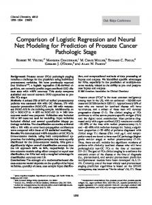
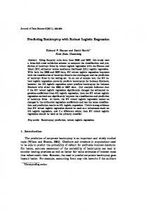
Indian diabetes (250/250/268), ionosphere (100/100/151), Haberman’s survival (250/250/268) and Wisconsin diagnostic breast cancer (WDBC) (100/100/369). During each iteration, a data set was randomly divided into training, validation and testing sets. The mean entropy loss for each method was recorded using only the test data; the penalty parameters were inferred with a grid search algorithm using the validation data. The entire procedure was repeated for 1000 iterations for each data set. Figure 2 depicts the mean entropy loss of the four methods tested. As with simulated data, the penalized regression methods outperformed stepwise regression in each simulation The performance difference is most evident on the WDBC dataset which contained a moderate number of predictor variables (p ≈ 30). In all experiments, the penalized regression methods performed roughly equally well, with ridge regression slightly outperforming LASSO and elastic net on the WDBC data. We also briefly compared the Bayesian LASSO [4] with the standard LASSO implementation using the UCI-MLR data sets. The Bayesian LASSO outperformed the standard LASSO in terms of mean entropy loss in all four data sets; interestingly, the parameter estimates of the two methods were relatively close. Figure 3 depicts the the Bayesian coefficient estimates for Haberman’s survival data and the WDBC data set. The behaviour of the LASSO shrinkage prior is clearly evident; the Bayesian estimates are much smaller than the maximum likelihood estimates and correspond to models with significantly better prediction accuracy. The maximum likelihood estimates for the WDBC data set were quite large and are not shown in Figure 3(b) for reasons of clarity. Therefore, the Bayesian LASSO should be preferred over the regular LASSO as it provides better prediction accuracy and an automatic estimate of the penalty parameter.

Review of modern logistic regression methods 0.65

9

1.4

1.2

0.6

Mean entropy loss

Mean entropy loss

1 0.55

0.5

0.8

0.6

0.45 0.4

0.4

0.2 Stepwise

Ridge

LASSO

Elastic Net

Stepwise

Ridge

Methods

LASSO

Elastic Net

Methods

(a) Pima

(b) Ionosphere

0.75 0.8 0.7

Mean entropy loss

Mean entropy loss

0.6 0.65

0.6

0.4

0.2

0.55

0

0.5

0.45

−0.2 Stepwise

Ridge

LASSO Methods

(c) Haberman

Elastic Net

Stepwise

Ridge

LASSO

Elastic Net

Methods

(d) WDBC

Fig. 2. Mean entropy loss performance of all methods on four real data sets from the UCI Machine Learning repository

6

Conclusion

This paper has compared stepwise regression, ridge regression, the LASSO and the elastic net using both real and simulated data. In all scenarios, penalized logistic regression was found to be superior to stepwise regression. Of the three penalized regression methods, the elastic net is recommended as it automatically handles data with various sparsity patterns as well as correlated groups of regressors. Additionally, the Bayesian LASSO was found to be superior to the regular LASSO in terms prediction accuracy in all real data tests. This is in agreement with previous research comparing Bayesian and standard penalized regression methods on linear models.

Acknowledgments. The authors would like to thank Robert B. Gramacy for providing his Bayesian logistic regression simulation source code.

100

Review of modern logistic regression methods

10

10

MLE

MLE MAP

0

posterior

−5 −20

−100

−15

−50

−10

posterior

0

50

5

MAP

mu

b1

b2 coefficients

(a) Haberman

b3

mu

b2

b4

b6

b8 b10

b13

b16

b19

b22

b25

b28

coefficients

(b) WDBC

Fig. 3. Regression coefficients estimated by Bayesian sampling for two real data sets

References 1. Bunea, F.: Honest variable selection in linear and logistic regression models via ℓ1 and ℓ1 + ℓ2 penalization. Electronic Journal of Statistics 2, 1153–1194 (2008) 2. Cessie, S.L., Houwelingen, J.C.V.: Ridge estimators in logistic regression. Journal of the Royal Statistical Society (Series C) 41(1), 191–201 (1992) 3. Genkin, A., Lewis, D.D., Madigan, D.: Large-scale Bayesian logistic regression for text categorization. Technometrics 49(3), 291–304 (2007) 4. Gramacy, R.B., Polson, N.G.: Simulation-based regularized logistic regression (2010), arXiv:1005.3430v1 5. Hesterberg, T., Choi, N.H., Meier, L., Fraley, C.: Least angle and ℓ1 penalized regression: A review. Statistics Survey 2, 61–93 (2008) 6. Hoerl, A., Kennard, R.: Ridge regression. In: Encyclopedia of Statistical Sciences, vol. 8, pp. 129–136. Wiley, New York (1988) 7. Holmes, C.C., Held, L.: Bayesian auxiliary variable models for binary and multinomial regression. Bayesian Analysis 1(1), 145–168 (2006) 8. James, G.M., Radchenko, P.: A generalized Dantzig selector with shrinkage tuning. Biometrika 96(2), 323–337 (June 2009) 9. O’Brien, S.M., Dunson, D.B.: Bayesian multivariate logistic regression. Biometrics 60(3), 739–746 (2004) 10. Scott, S.L.: Data augmentation, frequentist estimation, and the Bayesian analysis of multinomial logit models. Statistical Papers (to appear) 11. Tibshirani, R.: Regression shrinkage and selection via the lasso. Journal of the Royal Statistical Society (Series B) 58(1), 267–288 (1996) 12. Zou, H., Hastie, T.: Regularization and variable selection via the elastic net. Journal of the Royal Statistical Society (Series B) 67(2), 301–320 (2005)