Jun 3, 1997 - Master of Science in Electrical Engineering and Computer Science at the ... Nancy Lynch. NEC Professor of Software Science and Engineering ...... and conducts a successful round, there are (n2) messages in the channels which are ...... Technical Memo MIT/LCS/TM-487.b, Lab. for Computer Science, MIT,.
Revisiting the Paxos Algorithm by
Roberto De Prisco Laurea in Computer Science (1991) University of Salerno, Italy
Submitted to the Department of Electrical Engineering and Computer Science in partial ful llment of the requirements for the degree of
Master of Science in Electrical Engineering and Computer Science at the MASSACHUSETTS INSTITUTE OF TECHNOLOGY June 3, 1997 Revised August 1998
c Massachusetts Institute of Technology. All rights reserved.
Author . . . . . . . . . . . . . . . . . . . . . . . . . . . . . . . . . . . . . . . . . . . . . . . . . . . . . . . . . . . . . . Department of Electrical Engineering and Computer Science June 3, 1997 Certi ed by. . . . . . . . . . . . . . . . . . . . . . . . . . . . . . . . . . . . . . . . . . . . . . . . . . . . . . . . . . Prof. Nancy Lynch NEC Professor of Software Science and Engineering Thesis Supervisor Accepted by . . . . . . . . . . . . . . . . . . . . . . . . . . . . . . . . . . . . . . . . . . . . . . . . . . . . . . . . . Prof. Arthur C. Smith Chairman, Department Committee on Graduate Theses
2
Revisiting the Paxos Algorithm by Roberto De Prisco Submitted to the Department of Electrical Engineering and Computer Science on June 3, 1997, in partial ful llment of the requirements for the degree of Master of Science in Electrical Engineering and Computer Science
Abstract
The paxos algorithm is an e�cient and highly fault-tolerant algorithm, devised by Lamport, for reaching consensus in a distributed system. Although it appears to be practical, it seems to be not widely known or understood. This thesis contains a new presentation of the paxos algorithm, based on a formal decomposition into several interacting components. It also contains a correctness proof and a time performance and fault-tolerance analysis. The presentation is built upon a general timed automaton (GTA) model. The correctness proof uses automaton composition and invariant assertion methods. The time performance and fault-tolerance analysis is conditional on the stabilization of the underlying physical system behavior starting from some point in an execution. In order to formalize this stabilization, a special type of GTA called a Clock GTA is de ned. Thesis Supervisor: Prof. Nancy Lynch Title: NEC Professor of Software Science and Engineering
Acknowledgments I would like to thank my advisor Nancy Lynch. Her constant support throughout this work, her help for my understanding of the subject and the writing of the thesis, her thorough review of various revisions of the manuscript, substantially improved the overall quality of the thesis. I also thank Nancy for her patience in explaining me many times the things that I did not understand readily. In particular I am grateful to her for teaching me the di�erence between \that" and \which", that (or which?) is something I still have to understand! I would also like to thank Butler Lampson for useful discussions and suggestions. Butler also has written the 6.826 Principles of Computer System handout that provides a description of paxos; that handout provided the basis for the work in this thesis. I would like to thank Alan Fekete, Victor Luchangco, Alex Shvartsman and Mandana Vaziri for reading parts of the thesis and Atul Adya and Arvind Parthasarathi for useful discussions.
Contents 1 Introduction
7
2 Models 2.1 2.2 2.3 2.4 2.5 2.6
Overview . . . . . . . . . . . . . . . The basic I/O automata model . . The MMT automaton model. . . . The GT automaton model . . . . . The Clock GT automaton model . Composition of automata . . . . . . 2.6.1 Composition of BIOA. . . . 2.6.2 Composition of MMTA. . . 2.6.3 Composition of GTA. . . . . 2.6.4 Composition of Clock GTA. 2.7 Bibliographic notes . . . . . . . . .
. . . . . . . . . . .
. . . . . . . . . . .
. . . . . . . . . . .
. . . . . . . . . . .
. . . . . . . . . . .
. . . . . . . . . . .
. . . . . . . . . . .
. . . . . . . . . . .
. . . . . . . . . . .
. . . . . . . . . . .
. . . . . . . . . . .
. . . . . . . . . . .
. . . . . . . . . . .
. . . . . . . . . . .
. . . . . . . . . . .
. . . . . . . . . . .
. . . . . . . . . . .
. . . . . . . . . . .
. . . . . . . . . . .
16 16 18 19 21 23 29 29 32 33 35 35
3 The distributed setting
36
4 The consensus problem
44
3.1 Processes . . . . . . . . . . . . . . . . . . . . . . . . . . . . . . . . . 3.2 Channels . . . . . . . . . . . . . . . . . . . . . . . . . . . . . . . . . . 3.3 Distributed systems . . . . . . . . . . . . . . . . . . . . . . . . . . . .
4.1 Overview . . . . . . . . . . . . . . . . . . . . . . . . . . . . . . . . . . 4.2 Formal de nition . . . . . . . . . . . . . . . . . . . . . . . . . . . . . 5
37 38 41
44 47
4.3 Bibliographic notes . . . . . . . . . . . . . . . . . . . . . . . . . . . .
48
5 Failure detector and leader elector
50
6 The paxos algorithm
61
5.1 A failure detector . . . . . . . . . . . . . . . . . . . . . . . . . . . . . 5.2 A leader elector . . . . . . . . . . . . . . . . . . . . . . . . . . . . . . 5.3 Bibliographic notes . . . . . . . . . . . . . . . . . . . . . . . . . . . .
6.1 Overview . . . . . . . . . . . . . . 6.2 Automaton basicpaxos . . . . . 6.2.1 Overview . . . . . . . . . 6.2.2 The code . . . . . . . . . . 6.2.3 Partial Correctness . . . . 6.2.4 Analysis of Sbpx . . . . . 6.3 Automaton Spax . . . . . . . . . 6.4 Correctness and analysis of Spax 6.5 Messages . . . . . . . . . . . . . . 6.6 Concluding remarks . . . . . . . .
7 The multipaxos algorithm 7.1 7.2 7.3 7.4 7.5
Overview . . . . . . . . . . . . . Automaton multibasicpaxos. Automaton multistarteralg Correctness and analysis . . . . Concluding remarks . . . . . . .
8 Application to data replication
8.1 Overview . . . . . . . . . . . . . 8.2 Sequential consistency . . . . . 8.3 Using multipaxos . . . . . . . 8.3.1 The code . . . . . . . . . 8.3.2 Correctness and analysis
. . . . . . . . . . 6
. . . . . . . . . . . . . . . . . . . .
. . . . . . . . . . . . . . . . . . . .
. . . . . . . . . . . . . . . . . . . .
. . . . . . . . . . . . . . . . . . . .
. . . . . . . . . . . . . . . . . . . .
. . . . . . . . . . . . . . . . . . . .
. . . . . . . . . . . . . . . . . . . .
. . . . . . . . . . . . . . . . . . . .
. . . . . . . . . . . . . . . . . . . .
. . . . . . . . . . . . . . . . . . . .
. . . . . . . . . . . . . . . . . . . .
. . . . . . . . . . . . . . . . . . . .
. . . . . . . . . . . . . . . . . . . .
. . . . . . . . . . . . . . . . . . . .
. . . . . . . . . . . . . . . . . . . .
. . . . . . . . . . . . . . . . . . . .
. . . . . . . . . . . . . . . . . . . .
. . . . . . . . . . . . . . . . . . . .
. . . . . . . . . . . . . . . . . . . .
50 56 59
. 61 . 64 . 64 . 70 . 80 . 91 . 97 . 100 . 104 . 105 . . . . . . . . . .
107
107 108 118 119 119
122
122 123 124 126 130
8.4 Concluding remarks . . . . . . . . . . . . . . . . . . . . . . . . . . . . 132
9 Conclusions
134
A Notation
138
7
List of Figures 2-1 An I/O automaton. . . . . . . . . . . . . . . . . . . . . . . . . . . . .
21
3-1 Automaton channeli;j . . . . . . . . . . . . . . . . . . . . . . . . . . 3-2 The communication system Scha . . . . . . . . . . . . . . . . . . . .
42 45
5-1 5-2 5-3 5-4
Automaton detector for process i . . . . The system Sdet . . . . . . . . . . . . . . Automaton leaderelector for process i The system Slea . . . . . . . . . . . . . .
. . . .
54 55 60 61
6-1 6-2 6-3 6-4 6-5 6-6 6-7 6-8 6-9 6-10 6-11
paxos: process i. . . . . . . . . . . . . . . . . . . . . . . . . . . . . . basicpaxos: Messages. . . . . . . . . . . . . . . . . . . . . . . . . .
66 66 69 72 74 75 76 77 78 84 102
. . . .
. . . .
Exchange of messages . . . . . . . . . . . . . . Choosing the values of rounds. . . . . . . . . . Automaton bpleader for process i (part 1) . Automaton bpleader for process i (part 2) . Automaton bpagent for process i . . . . . . Automaton bpsuccess for process i (part 1) . Automaton bpsuccess for process i (part 2) . History variables. . . . . . . . . . . . . . . . . Automaton starteralg for process i . . . .
. . . .
. . . . . . . . .
. . . .
. . . . . . . . .
. . . .
. . . . . . . . .
. . . .
. . . . . . . . .
. . . .
. . . . . . . . .
. . . .
. . . . . . . . .
. . . .
. . . . . . . . .
. . . .
. . . . . . . . .
. . . .
. . . . . . . . .
. . . .
. . . . . . . . .
. . . .
. . . . . . . . .
. . . .
. . . . . . . . .
. . . . . . . . .
7-1 Automaton bmpleader for process i (part 1) . . . . . . . . . . . . . 115 7-2 Automaton bmpleader for process i (part 2) . . . . . . . . . . . . . 116 7-3 Automaton bmpagent for process i . . . . . . . . . . . . . . . . . . . 117 8
7-4 7-5 7-6 7-7
Automaton bmpsuccess for process i (part 1) . . . . Automaton bmpsuccess for process i (part 2) . . . . Automaton multistarteralg for process i (part 1) Automaton multistarteralg for process i (part 2)
. . . .
. . . .
. . . .
. . . .
. . . .
. . . .
. . . .
. . . .
. . . .
118 119 123 124
8-1 Automaton datareplication for process i (part 1) . . . . . . . . . 130 8-2 Automaton datareplication for process i (part 2) . . . . . . . . . 131 8-3 Data replication . . . . . . . . . . . . . . . . . . . . . . . . . . . . . . 136
9
Chapter 1 Introduction Reaching consensus is a fundamental problem in distributed systems. Given a distributed system in which each process1 starts with an initial value, to solve a consensus problem means to give a distributed algorithm that enables each process to eventually output a value of the same type as the input values, in such a way that three conditions, called agreement, validity and termination, hold. There are di�erent definitions of the problem depending on what these conditions require. The agreement condition states requirements about the way processes need to agree (e.g., \no two di�erent outputs occur"). The validity condition states requirements about the relation between the input and the output values (e.g., \any output value must belong to the set of initial values"). The termination condition states requirements about the termination of an algorithm that solves the problem (e.g., \each non-faulty process eventually outputs a value"). Distributed consensus has been extensively studied; a good survey of early results is provided in [17]. We refer the reader to [35] for a more up-to-date treatment of consensus problems. We remark that the words \process" and \processor" are often used as synonyms. The word \processor" is more appropriate when referring to a physical component of a distributed system. A physical processor is often viewed as consisting of several logical components, called \processes". Processes are composed to describe larger logical components, and the resulting composition is also called a process. Thus the whole physical processor can be identi ed with the composition of all its logical components. Whence the word \process" can also be used to indicate the physical processor. In this thesis we use the word \process" to mean either a physical processor or a logical component of it. The distinction either is unimportant or should be clear from the context. 1
10
Consensus problems arise in many practical situations, such as, for example, distributed data replication, distributed databases and ight control systems. Data replication is used in practice to provide high availability: having more than one copy of the data allows easier access to the data, i.e., the nearest copy of the data can be used. However, consistency among the copies must be maintained. A consensus algorithm can be used to maintain consistency. A practical example of the use of data replication is an airline reservation system. The data consists of the current booking information for the ights and it can be replicated at agencies spread over the world. The current booking information can be accessed at any of the replicas. Reservations or cancellations must be agreed upon by all the copies. In a distributed database, the consensus problem arises when a collection of processes participating in the processing of a distributed transaction has to agree on whether to commit or abort the transaction, that is, make the changes due to the transaction permanent or discard the changes. A common decision must be taken to avoid inconsistencies. A practical example of the use of distributed transactions is a banking system. Transactions can be done at any bank location or ATM machine, and the commitment or abortion of each transaction must be agreed upon by all the bank locations or ATM machines involved. In a ight control system, the consensus problem arises when the ight surface and airplane control systems have to agree on whether to continue or abort a landing in progress or when the control systems of two approaching airplanes need to modify the air routes to avoid collision. Various theoretical models of distributed systems have been considered. A general classi cation of models is based on the kind of communications allowed between processes of the distributed system. There are two ways by which processes communicate: by passing messages over communication channels or using a shared memory. In this thesis we focus on message-passing models. A wide variety of message-passing models can be used to represent distributed systems. They can be classi ed by the network topology, the synchrony of the system and the failures allowed. The network topology describes which processes can send 11
messages directly to which other processes and it is usually represented by a graph in which nodes represent processes and edges represent direct communication channels. Often one assumes that a process knows the entire network; sometimes one assumes that a process has only a local knowledge of the network (e.g., each process knows only the processes for which it has a direct communication channel). About synchrony, several model variations, ranging from the completely asynchronous setting to the completely synchronous one, can be considered. A completely asynchronous model is one with no concept of real time. It is assumed that messages are eventually delivered and processes eventually respond, but it may take arbitrarily long. In partially synchronous systems some timing assumptions are made. For example, upper bounds on the time needed for a process to respond and for a message to be delivered hold. These upper bounds are known by the processes and processes have some form of real-time clock to take advantage of the time bounds. In completely synchronous systems, the computation proceeds in rounds in which steps are taken by all the processes. Failures may concern both communication channels and processes. In partially synchronous models, messages are supposed to be delivered and processes are expected to act within some time bounds; a timing failure is a violation of these time bounds. Communication failures can result in loss of messages. Duplication and reordering of messages may be considered failures, too. The weakest assumption made about process failures is that a faulty process has an unrestricted behavior. Such a failure is called a Byzantine failure. More restrictive models permit only omission failures, in which a faulty process fails to send some messages. The most restrictive models allow only stopping failures, in which a failed process simply stops and takes no further actions. Some models assume that failed processes can be restarted. Often processes have some form of stable storage that is not a�ected by a stopping failure; a stopped process is restarted with its stable storage in the same state as before the failure and with every other part of its state restored to some initial values. In the absence of failures, distributed consensus problems are easy to solve: it is enough to exchange information about the initial values of the processes and use a 12
common decision rule for the output in order to satisfy both agreement and validity. Failures complicate the matter, so that distributed consensus can even be impossible to achieve. The di�culties depend upon the distributed system model considered and the exact de nition of the problem (i.e., the agreement, validity and termination conditions). Real distributed systems are often partially synchronous systems subject to process, channel and timing failures and process recoveries. Today's distributed systems occupy larger and larger physical areas; the larger the physical area spanned by the distributed system, the harder it is to provide synchrony. Physical components are subject to failures. When a failure occurs, it is likely that, some time later, the problem is xed, restoring the failed component to normal operation. Moreover, though timely responses can usually be provided in real distributed systems, the possibility of process and channel failures makes it impossible to guarantee that timing assumptions are always satis ed. Thus real distributed systems su�er timing failures. Any practical consensus algorithm needs to consider all the above practical issues. Moreover, the basic safety properties must not be a�ected by the occurrence of failures. Also, the performance of the algorithm should be good when there are no failures. paxos is an algorithm devised by Lamport [29] that solves the consensus problem.
The model considered is a partially synchronous distributed system where each process has a direct communication channel with each other process. The failures allowed are timing failures, loss, duplication and reordering of messages and process stopping failures. Process recoveries are considered; some stable storage is needed. paxos is guaranteed to work safely, that is, to satisfy agreement and validity, regardless of process, channel and timing failures and process recoveries. When the distributed system stabilizes, meaning that there are no failures nor process recoveries and a majority of the processes are not stopped, for a su�ciently long time, termination is achieved; the performance of the algorithm when the system stabilizes is good. In [29] there is also presented a variation of paxos that considers multiple concurrent runs of paxos when consensus has to be reached on a sequence of values. We call this variation the 13
multipaxos algorithm2.
The basic idea of the paxos algorithm is to have processes propose values until one of the value is accepted by a majority of the processes: that value is the nal output value. Any process may propose a value by initiating a round for that value. The process initiating a round is the leader of that round. Rounds are guaranteed to satisfy agreement and validity. A successful round, that is, a round in which a value is accepted by a majority of the processes, results in the termination of the algorithm. However a successful round is guaranteed to be conducted only when the distributed system stabilizes. Basically paxos keeps starting rounds while the system is not stable, but when the system stabilizes, a successful round is conducted. Though failures may force the algorithm to repeatedly start new rounds, a single round is not costly: it uses O(n) messages, where n is the number of processes, and constant time. Thus, paxos has good fault-tolerance properties and when the system is stable combines those fault-tolerance properties with the performance of an e�cient algorithm, so that it can be useful in practice. In the original paper [29], the paxos algorithm is described as the result of discoveries of archaeological studies of an ancient Greek civilization. That paper contains a sketch of a proof of correctness and a discussion of the performance analysis. The style used for the description of the algorithm often diverts the reader's attention. Because of this, we found the paper hard to understand and we suspect that others did as well. Indeed the paxos algorithm, even though it appears to be a practical and elegant algorithm, seems not widely known or understood, either by distributed systems researchers or distributed computing theory researchers. This thesis contains a new, detailed presentation of the paxos algorithm, based on a formal decomposition into several interacting components. It also contains a correctness proof and a time performance and fault-tolerance analysis. The multipaxos algorithm is also described together with an application to data replication. 2 paxos is the name of the ancient civilization studied in [29]. The actual algorithm is called the \single-decree synod" protocol and its variation for multiple consensus is called the \multi-decree parliament" protocol. We take the liberty of using the name paxos for the single-decree synod protocol and the name multipaxos for the multi-decree parliament protocol.
14
The formal framework used for the presentation is provided by Input/Output automata models. Input/Output automata are simple state machines with transitions labelled with actions. They are suitable for describing asynchronous and partially synchronous distributed systems. The basic I/O automaton model, introduced by Lynch and Tuttle [37], is suitable for modelling asynchronous distributed systems. For our purposes, we will use the general timed automaton (GTA) model, introduced by Lynch and Vandraager [38, 39, 40]3, which has formal mechanisms to represent the passage of time and is suitable for modelling partially synchronous distributed systems. The correctness proof uses automaton composition and invariant assertion methods. Composition is useful for representing a system using separate components. This split representation is helpful in carrying out the proofs. We provide a modular presentation of the paxos algorithm, obtained by decomposing it into several components. Each one of these components copes with a speci c aspect of the problem. In particular there is a \failure detector" module that detects process failures and recoveries. There is a \leader elector" module that copes with the problem of electing a leader; processes elected leader by this module, start new rounds for the paxos algorithm. The paxos algorithm is then split into a basic part that ensures agreement and validity and an additional part that ensures termination when the system stabilizes; the basic part of the algorithm, for the sake of clarity of presentation, is further subdivided into three components. The correctness of each piece is proved by means of invariants, i.e., properties of system states that are always true in an execution. The key invariants we use in our proof are the same as in [31, 32]. The time performance and fault-tolerance analysis is conditional on the stabilization of the system behavior starting from some point in an execution. While it is easy to formalize process and channel failures, dealing formally with timing failures is harder. To cope with this problem, this thesis introduces a special type of GTA called a Clock GTA. The Clock GTA is a GTA augmented with a simple way of forThe term \general timed automaton" was not used in these papers; it was introduced in the book by Lynch [35]. 3
15
malizing timing failures. Using the Clock GTA we provide a technique for practical time performance analysis based on the stabilization of the physical system. A detailed description of the multipaxos protocol is also provided. As an example of an application, the use of multipaxos to implement a data replication algorithm is presented. With multipaxos the high availability of the replicated data is combined with high fault tolerance. This is not trivial, since having replicated copies implies that consistency has to be guaranteed and this may result in low fault tolerance. Independent work related to paxos has been carried out. The algorithms in [11, 34] have similar ideas. The algorithm of Dwork, Lynch and Stockmeyer [11] also uses rounds conducted by a leader, but the rounds are conducted sequentially, whereas in paxos a leader can start a round at any time and multiple simultaneous leaders are allowed. The strategy used in each round by the algorithm of [11] is somewhat di�erent from the one used by paxos. Moreover the distributed model of [11] does not consider process recoveries. The time analysis provided in [11] is conditional on a \global stabilization time" after which process response times and message delivery times satisfy the time assumptions. This is similar to our analysis. (A similar time analysis, applied to a di�erent problem, can be found in [16].) multipaxos can be easily used to implement a data replication algorithm. In [34] a data replication algorithm is provided. It incorporates ideas similar to the ones used in paxos. paxos bears some similarities with the standard three-phase commit protocol: both require, in each round, an exchange of 5 messages. However the standard commit protocol requires a reliable leader elector while paxos does not. Moreover paxos sends information on the value to agree on, only in the third message of a round, while the commit protocol sends it in the rst message; because of this, multipaxos can exchange the rst two messages only once for many instances and use only the exchange of the last three messages for each individual consensus problem while such a strategy cannot be used with the three-phase commit protocol. In the class notes of the graduate level Principles of Computer Systems course [31] taught at MIT, a description of paxos is provided using a speci cation language called 16
SPEC. The presentation in [31] contains the description of how a round of paxos is conducted. The leader election problem is not considered. Timing issues are not addressed; for example, the problem of starting new rounds is not considered. A proof of correctness, written also in SPEC, is outlined. Our presentation di�ers from that of [31] in the following aspects: it is based on I/O automata models rather than on a programming language; it provides all the details of the algorithm; it provides a modular description of the algorithm, including auxiliary parts such as a failure detector module and a leader elector module; along with the proof of correctness, it provides a performance and fault-tolerance analysis. In [32] Lampson provides an overview of the paxos algorithm together with the key points for proving the correctness of the algorithm. In [43] the clock synchronization problem has been studied; the solution provided there introduces a new type of GTA, called the mixed automaton model. The mixed automaton is similar to our Clock automaton with respect to the fact that both try to formally handle the local clocks of processes. However while the mixed automaton model is used to describe synchronization of the local clocks, the Clock GTA automaton is used to model good timing behavior and thus does not need to cope with synchronization.
Summary of contributions. This thesis provides a new, detailed and modular
description of the paxos algorithm, a correctness proof and a time performance analysis. The multipaxos algorithm is described and an application to data replication is provided. This thesis also introduces a special type of GTA model, called the Clock GTA model, and a technique for practical time performance analysis when the system stabilizes.
Organization. This thesis is organized as follows. In Chapter 2 we provide a
description of the I/O automata models and in particular we introduce the Clock GTA model. In Chapter 3 we discuss the distributed setting we consider. Chapter 4 gives a formal de nition of the consensus problem we consider. Chapter 5 is devoted 17
to the design of a simple failure detector and a simple leader elector which will be used to give an implementation of paxos. Then in Chapter 6 we describe the paxos algorithm, prove its correctness and analyze its performance. In Chapter 7 we describe the multipaxos algorithm. Finally in Chapter 8 we discuss how to use multipaxos to implement a data replication algorithm. Chapter 9 contains the conclusions.
18
Chapter 2 Models In this chapter we describe the I/O automata models we use in this thesis. Section 2.1 presents an overview of the automata models. Then, Section 2.2 describes the basic I/O automaton model, which is used in Section 2.3 to describe the MMT automaton model. Section 2.4 describes the general timed automaton model. In Section 2.5 the Clock GT automaton is introduced; Section 2.5 provides also a technique to transform an MMTA into a Clock GTA. Section 2.6 describes how automata are composed.
2.1 Overview The I/O automata models are formal models suitable for describing asynchronous and partially synchronous distributed systems. Various I/O automata models have been developed so far (see, for example, [35]). The simplest I/O automata model does not consider time and thus it is suitable for describing asynchronous systems. We remark that in the literature this simple I/O automata model is referred to as the \I/O automaton model". However we prefer to use the general expression \I/O automata models" to indicate all the I/O automata models, henceforth we refer to the simplest one as the \basic I/O automaton model" (BIOA for short). The BIOA model was developed by Lynch and Tuttle [37]. Two extensions of the BIOA model that provide formal mechanisms to handle the passage of time and thus are suitable for describing partially synchronous distributed systems, are the MMT automaton 19
(MMTA for short), developed by Merritt, Modugno and Tuttle [42] and the general timed automaton (GT automaton or GTA for short) developed by Lynch and Vaandrager [38, 39, 40]. The MMTA is a special case of GTA, and thus it can be regarded as a notation for describing some GT automata. In this thesis we introduce a particular type of GTA that we call \Clock GTA". The Clock GTA is suitable for describing partially synchronous distributed systems with processors having local clocks; thus it is suitable for describing timing assumptions. In this thesis we use the GTA model and in particular the Clock GT automaton model. However, we use the MMT automaton model to describe some of the Clock GTAs1 ; this is possible because an MMTA is a particular type of GTA; there is a standard technique that transforms an MMTA into a GTA and we specialize this technique in order to transform an MMT automaton into a Clock GTA. An I/O automaton is a simple type of state machine in which transitions are associated with named actions. These actions are classi ed into categories, namely input, output, internal and, for the timed models, time-passage. Input and output actions are used for communication with the external environment, while internal actions are local to the automaton. The time-passage actions are intended to model the passage of time. The input actions are assumed not to be under the control of the automaton, that is, they are controlled by the external environment which can force the automaton to execute the input actions. Internal and output actions are controlled by the automaton. The time-passage actions are also controlled by the automaton. As an example, we can consider an I/O automaton that models the behavior of a process involved in a consensus problem. Figure 2-1 shows the typical interface (that is, input and output actions) of such an automaton. The automaton is drawn as a circle, input actions are depicted as incoming arrows and output actions as outcoming arrows (internal actions are hidden since they are local to the automaton). The reason why we use MMT automata to describe some of our Clock GT automata is that MMT automata code is simpler. We use MMTA to describe the parts of the algorithm that can run asynchronously and we use the time bounds only for the analysis. 1
20
Init(v)
Decide(v)
I/O automaton
Send(m)
Receive(m)
Figure 2-1: An I/O automaton. The automaton receives inputs from the external world by means of action Init(v), which represents the receipt of an input value v and conveys outputs by means of action Decide(v) which represents a decision of v. Actions Send(m) and Receive(m) are supposed to model the communication with other automata.
2.2 The basic I/O automata model A signature S is a triple consisting of three disjoint sets of actions: the input actions, in (S ), the output actions, out (S ), and the internal actions, int (S ). The external actions, ext (S ), are in (S ) [ out (S ); the locally controlled actions, local (S ), are out (S ) [ int (S ); and acts (S ) consists of all the actions of S . The external signature, extsig (S ), is de ned to be the signature (in (S ); out (S ); ;). The external signature is also referred to as the external interface. A basic I/O automaton (BIOA for short) A, consists of ve components:
� sig (A), a signature � states (A), a (not necessarily nite) set of states � start (A), a nonempty subset of states (A) known as the start states or initial states
� trans (A), a state-transition relation, where trans (A) � states (A) � 21
acts (sig (A)) � states (A); this must have the property that for every state s and every input action �, there is a transition (s; �; s0) 2 trans (A)
� tasks (A), a task partition, which is an equivalence relation on local (sig (A)) having at most countably many equivalence classes
Often acts (A) is used as shorthand for acts (sig (A)), and similarly in (A), and so on. An element (s; �; s0) of trans (A) is called a transition , or step , of A. If for a particular state s and action �, A has some transition of the form (s; �; s0), then we say that � is enabled in s. Input actions are enabled in every state. The fth component of the I/O automaton de nition, the task partition tasks (A), should be thought of as an abstract description of \tasks," or \threads of control," within the automaton. This partition is used to de ne fairness conditions on an execution of the automaton; roughly speaking, the fairness conditions say that the automaton must continue, during its execution, to give fair turns to each of its tasks. An execution fragment of A is either a nite sequence, s0 ; �1; s1; �2 ; : : : ; �r ; sr , or an in nite sequence, s0 ; �1; s1; �2 ; : : : ; �r ; sr ; : : : , of alternating states and actions of A such that (sk ; �k+1; sk+1) is a transition of A for every k � 0. Note that if the sequence is nite, it must end with a state. An execution fragment beginning with a start state is called an execution. The length of a nite execution fragment � = s0; �1 ; s1; �2; : : : ; �r ; sr is r. The set of executions of A is denoted by execs (A). A state is said to be reachable in A if it is the nal state of a nite execution of A. The trace of an execution � of A, denoted by trace (�), is the subsequence of � consisting of all the external actions. A trace of A is a trace of an execution of A. The set of traces of A is denoted by traces (A).
2.3 The MMT automaton model. An MMT timed automaton model is obtained simply by adding to the BIOA model lower and upper bounds on the time that can elapse before an enabled action is executed. Formally an MMT automaton consists of a BIOA and a boundmap b. A 22
boundmap b is a pair of mappings, lower and upper which give lower and upper bounds for all the tasks. For each task C , it is required that 0 � lower(C ) � upper(C ) � 1 and that lower(C ) < 1. The bounds lower(C ) and upper(C ) are respectively, a lower bound and an upper bound on the time that can elapse before an enabled action belonging to C is executed. A timed execution of an MMT automaton B = (A; b) is de ned to be a nite sequence � = s0 , (�1 ; t1), s1 , (�2 ; t2); : : : ; (�r ; tr ), sr or an in nite sequence � = s0, (�1 ; t1), s1 , (�2 ; t2); : : : ; (�r ; tr ), sr ; : : : , where the s's are states of the I/O automaton A, the �'s are actions of A, and the t's are times in R �0 . It is required that the sequence s0 ; �1; s1; : : : |that is, the sequence � with the times ignored|be an ordinary execution of I/O automaton A. It is also required that the successive times tr in � be nondecreasing and that they satisfy the lower and upper bound requirements expressed by the boundmap b. De ne r to be an initial index for a task C provided that C is enabled in sr and one of the following is true: (i) r = 0; (ii) C is not enabled in sr?1; (iii) �r 2 C . The initial indices represent the points at which we begin to measure the time bounds of the boundmap. For every initial index r for a task C , it is required that the following conditions hold. (Let t0 = 0.) Upper bound condition: If there exists k > r with tk > tr + upper(C ), then there exists k0 > r with tk � tr + upper(C ) such that either �k 2 C or C is not enabled in sk . Lower bound condition: There does not exist k > r with tk < tr + lower(C ) and �k 2 C . The upper bound condition says that, from any initial index for a task C , if time ever passes beyond the speci ed upper bound for C , then in the interim, either an action in C must occur, or else C must become disabled. The lower bound condition says that, from any initial index for C , no action in C can occur before the speci ed lower bound. The set of timed executions of B is denoted by texecs (B ). A state is said to be reachable in B if it is the nal state of some nite timed execution of B . 0
0
0
23
A timed execution is admissible provided that the following condition is satis ed:
Admissibility condition: If timed execution � is an in nite sequence, then the times of the actions approach 1. If � is a nite sequence, then in the nal state of �, if task C is enabled, then upper(C ) = 1. The admissibility condition says that time advances normally and that processing does not stop if the automaton is scheduled to perform some more work. The set of admissible timed executions of B is denoted by atexecs (B ). Notice that time bounds of the MMT substitute for the fairness conditions of a BIOA. The timed trace of a timed execution � of B , denoted by ttrace (�), is the subsequence of � consisting of all the external actions, each paired with its associated time. The admissible timed traces of B , which are denoted by attraces (B ), are the timed traces of admissible timed executions of B .
2.4 The GT automaton model The GTA model uses time-passage actions called � (t), t 2 R + to model the passage of time. The time-passage action � (t) represents the passage of time by the amount t. A timed signature S is a quadruple consisting of four disjoint sets of actions: the input actions in (S ), the output actions out (S ), the internal actions int (S ), and the time-passage actions. For a GTA
� the visible actions, vis (S ), are the input and output actions, in (S ) [ out (S ) � the external actions, ext (S ), are the visible and time-passage actions, vis (S ) [ f� (t) : t 2 R + g � the discrete actions, disc (S ), are the visible and internal actions, vis (S ) [ int (S ) � the locally controlled actions, local (S ), are the output and internal actions, out (S ) [ int (S ) 24
� acts (S ) are all the actions of S A GTA A consists of the following four components:
� sig (A), a timed signature � states (A), a set of states � start (A), a nonempty subset of states (A) known as the start states or initial states
� trans (A), a state transition relation, where trans (A) � states (A) � acts (sig (A)) � states (A); this must have the property that for every state s and every input action �, there is a transition (s; �; s0) 2 trans (A) Often acts (A) is used as shorthand for acts (sig (A)), and similarly in (A), and so on. An element (s; �; s0) of trans (A) is called a transition , or step , of A. If for a particular state s and action �, A has some transition of the form (s; �; s0), then we say that � is enabled in s. Since every input action is required to be enabled in every state, automata are said to be input-enabled. The input-enabling assumption means that the automaton is not able to somehow \block" input actions from occurring. There are two simple axioms that A is required to satisfy:
A1: If (s; � (t); s0) and (s0 ; � (t0); s00) are in trans (A), then (s; � (t+t0 ); s00) is in trans (A). A2: If (s; � (t); s0) 2 trans (A) and 0 < t0 < t, then there is a state s00 such that (s; � (t0); s00) and (s00; � (t ? t0 ); s0) are in trans (A). Axiom A1 allows repeated time-passage steps to be combined into one step, while Axiom A2 is a kind of converse to A1 that allows a time-passage step to be split in two. A timed execution fragment of a GTA, A, is de ned to be either a nite sequence � = s0; �1 ; s1; �2; : : : ; �r ; sr or an in nite sequence � = s0; �1 ; s1; �2; : : : ; �r ; sr ; : : : , where the s's are states of A, the �'s are actions (either input, output, internal, or time-passage) of A, and (sk ; �k+1; sk+1) is a step (or transition) of A for every k. Note 25
that if the sequence is nite, it must end with a state. The length of a nite execution fragment � = s0; �1; s1 ; �2; : : : ; �r ; sr is r. A timed execution fragment beginning with a start state is called a timed execution. Axioms A1 and A2, say that there is not much di�erence between timed execution fragments that di�er only by splitting and combining time-passage steps. Two timed execution fragments � and �0 are time-passage equivalent if � can be transformed into �0 by splitting and combining time-passage actions according to Axioms A1 and A2. If � is any timed execution fragment and �r is any action in �, then we say that the time of occurrence of �r is the sum of all the reals in the time-passage actions preceding �r in �. A timed execution fragment � is said to be admissible if the sum of all the reals in the time-passage actions in � is 1. The set of admissible timed executions of A is denoted by atexecs (A). A state is said to be reachable in A if it is the nal state of a nite timed execution of A. The timed trace of a timed execution fragment �, denoted by ttrace (�), is the sequence of visible events in �, each paired with its time of occurrence. The admissible timed traces of A, denoted by attraces (A), are the timed traces of admissible timed executions of A. We may refer to a timed execution simply as an execution. Similarly a timed trace can be referred to as a trace.
2.5 The Clock GT automaton model A Clock GTA is a GTA with a special component included in the state; this special variable is called Clock and it can assume values in R . The purpose of Clock is to model the local clock of the process. The only actions that are allowed to modify Clock are the time-passage actions � (t). When a time-passage action � (t) is executed by an automaton, the Clock is incremented by an amount of time t0 � 0 independent of the amount t of time speci ed by the time-passage action. Formally, beside Axioms A1 and A2, of a regular GTA, for a Clock GTA we 26
require that
A3: If (s; � (t); s0) is in trans (A), then (s; � (t~); s0), for any t~ > 0, is in trans (A). Hence a Clock GTA cannot keep track of the real time. Since the occurrence of the time-passage action � (t) represents the passage of (real) time by the amount t, by incrementing the variable Clock by an amount t0 di�erent from t we are able to model the passage of clock time by the amount t0 . As a special case, we have some time-passage actions in which t0 = t; in these cases the local clock of the process is running at the speed of real time. In the following and in the rest of the thesis, we use the notation s:x to denote the value of state component x in state s.
De nition 2.5.1 A step (sk?1; � (t); sk ) of a Clock GTA is called regular if sk :Clock ? sk?1:Clock = t; it is called irregular if it is not regular.
That is, a time-passage step executing action � (t) is regular if it increases Clock by t0 = t. In a regular time-passage step, the local clock is increased by the same amount as the real time, whereas in an irregular time-passage step � (t) that represents the passage of real time by the amount t, the local clock is increased either by t0 < t (the local clock is slower than the real time) or by t0 > t (the local clock is faster than the real time).
De nition 2.5.2 A timed execution fragment � of a Clock GTA is called regular if all the time-passage steps of � are regular. It is called irregular if it is not regular, i.e., if at least one of its time-passage steps is irregular.
In a partially synchronous distributed system processes are expected to respond and messages are expected to be delivered within given time bounds. A timing failure is a violation of these time bounds. An irregular time-passage step can model the occurrence of a timing failure in the following way. Assume that a particular process is supposed to execute some action within a given time bound and this time bound is modeled by restricting the time that can elapse with time-passage actions (this is 27
how GT automata are used to model partial synchrony). We can impose the same time bound on the clock time so that when time-passage action � (t) is executed the local clock of the particular process we are considered is actually incremented by an amount t0 so that the time bound on the local clock time is not violated. Clearly if t0 < t then it is possible that a violation of the time bound (with respect to real time) actually occurs. We remark that a time bound violation can actually be either an upper bound violation (a process or a channel is slower than expected) or a lower bound violation (a process or a channel is faster than expected). The latter can be modeled with a time-passage action � (t) that increments the clock time by an amount t0 , t0 > t. Though we have de ned a regular execution fragment so that it does not contain any of the timing failures, we remark that for the the scope of this thesis we actually need only that the former type of timing failures (upper bound) does not happen. That is, for the scope of this thesis, we could have de ned a regular step � (t) as one that increases the clock time by an amount t0, t0 � t. However, to not lose in generality, a regular step is de ned to rule out both kinds timing failures. Obviously, in a regular execution fragment there are no timing failures.
Transforming MMTA into Clock GTA. MMT automata are a special case of
GT automata. There is a standard transformation technique that given an MMTA produces an equivalent GTA, i.e., one that has the same external behavior (see Section 23.2.2 of [35]). Next, we show how to transform any MMT automaton (A; b) into an equivalent clock general timed automaton A0 = clockgen(A; b). Automaton A0 acts like automaton A, but the time bounds of the boundmap b are expressed as restrictions on the value that the local time can assume. The technique used is essentially the same as the one that transforms an MMTA into an equivalent GTA with some modi cations to handle the Clock variable. The transformation involves building clock time deadlines into the state and not allowing the clock time to pass beyond those deadlines while they are still in force. 28
The deadlines are set according to the boundmap b. New constraints on non-timepassage actions are added to express the lower bound conditions. Notice however, that all these constraints are on the clock time, while in the transformation of an MMTA into a GTA they are on the real time. More speci cally, the state of the underlying BIOA A is augmented with a Clock component, plus First(C ) and Last(C ) components for each task C . The First(C ) and Last(C ) components represent, respectively, the earliest and latest clock times at which the next action in task C is allowed to occur. The time-passage actions � (t) are also added. The First and Last components get updated by the various steps, according to the lower and upper bounds speci ed by the boundmap b. The time-passage actions � (t) have an explicit precondition saying that the clock time cannot pass beyond any of the Last(C ) values; this is because these represent deadlines for the various tasks. Restrictions are also added on actions in any task C , saying that the current clock time Clock must be at least as great as the lower bound First(C ). In more detail, the timed signature of A0 = clockgen(A; b) is the same as the signature of A, with the addition of the time-passage actions � (t), t 2 R + . Each state of A0 consists of the following components: basic 2 states (A), initially a start state of A Clock 2 R , initially arbitrary For each task C of A: First(C ) 2 R , initially Clock + lower(C ) if C is enabled in state basic, otherwise 0 Last(C ) 2 R [ f1g, initially Clock + upper(C ) if C is enabled in basic, otherwise 1
The transitions are de ned as follows. If � 2 acts(A), then (s; �; s0) 2 trans (A0) exactly if all the following conditions hold: 1. (s:basic; �; s0:basic) 2 trans (A). 29
2. s0:Clock = s:Clock. 3. For each C 2 tasks (A), (a) If � 2 C , then s:First(C ) � s:Clock. (b) If C is enabled in both s:basic and s0:basic and � 2= C , then s:First(C ) = s0 :First(C ) and s:Last(C ) = s0:Last(C ). (c) If C is enabled in s0:basic and either C is not enabled in s:basic or � 2 C , then s0:First(C ) = s:Clock + lower(C ) and s0:Last(C ) = s:Clock + upper(C ). (d) If C is not enabled in s0 :basic, then s0:First(C ) = 0 and s0:Last(C ) = 1. If � = � (t), then (s; �; s0) 2 trans (A0 ) exactly if all the following conditions hold: 1. s0:basic = s:basic. 2. s0:Clock � s:Clock. 3. For each C 2 tasks (A), (a) s0 :Clock � s:Last(C ). (b) s0 :First(C ) = s:First(C ) and s0:Last(C ) = s:Last(C ). It should be clear that the above transformation yields a Clock GTA and that for each task C , the lower and upper time bounds speci ed by the boundmap's components First(C ) and Last(C ) are transformed into lower and upper bounds on the clock time. More formally we have the following lemma.
Lemma 2.5.3 In any reachable state of clockgen(A; b) and for any task C of A, we
have that.
1. Clock � Last(C ). 2. If C is enabled, then Last(C ) � Clock + upper(C ). 3. First(C ) � Clock + lower(C ).
30
4. First(C ) � Last(C ).
If some of the timing requirements speci ed by b are trivial|that is, if some lower bounds are 0 or some upper bounds are 1|then it is possible to simplify the automaton clockgen(A; b) just by omitting mention of these components. In this thesis all the MMT automata have boundmaps that specify a lower bound of 0 and an upper bound of a xed constant `; thus the above general transformation could be simpli ed (by omitting mention of First(C ) and using ` instead of upper(C ), for any C ) for our purposes. In the following lemma we assume lower(C ) = 0 and upper(C ) = `. Informally the lemma states that if B = clockgen(A; b) is a clock GTA obtained by transforming an MMTA A with boundmap b, then the upper bounds on tasks of A speci ed by the boundmap b are not violated when B executes a regular execution fragment.
Lemma 2.5.4 Consider a regular execution fragment � of clockgen(A; b), starting
from a reachable state s0 and lasting for more than ` time. Assume that lower(C ) = 0 and upper(C ) = ` for each task C of automaton A. Then (i) any task C enabled in s0 either has a step or is disabled within ` time, and (ii) any new enabling of C has a subsequent step or disabling within ` time, provided that � lasts for more than ` time from the enabling of C .
Proof: Let us rst prove (i). Let C be a task enabled in state s0. By Lemma 2.5.3 we have that s0 :First(C ) � s0 :Clock � s0:Last(C ) and that s0:Last(C ) � s0 :Clock + `.
Since the execution is regular and lasts for more then ` time, within time `, Clock passes the value s0:Clock + `. But this cannot happen (since s0:Last(C ) � s0 :Clock + `) unless Last(C ) is increased, which means either C has a step or it is disabled within ` time. The proof of (ii) is similar. Let s be the state in which C becomes enabled. Then the proof is as before replacing s0 with s.
31
2.6 Composition of automata The composition operation allows an automaton representing a complex system to be constructed by composing automata representing simpler system components. The most important characteristic of the composition of automata is that properties of isolated system components still hold when those isolated components are composed with other components. The composition identi es actions with the same name in di�erent component automata. When any component automaton performs a step involving �, so do all component automata that have � in their signatures. Since internal actions of an automaton A are intended to be unobservable by any other automaton B , automaton A cannot be composed with automaton B unless the internal actions of A are disjoint from the actions of B . Moreover, A and B cannot be composed unless the sets of output actions of A and B are disjoint.
2.6.1 Composition of BIOA. Let I be an arbitrary nite index set2 . A nite countable collection fSigi2I of signatures is said to be compatible if for all i; j 2 I , i 6= j , the following hold3: 1. int (Si ) \ acts (Sj ) = ; 2. out (Si) \ out (Sj ) = ; A nite collection of automata is said to be compatible if their signatures are compatible. When we compose a collection of automata, output actions of the components become output actions of the composition, internal actions of the components become internal actions of the composition, and actions that are inputs to some components The composition operation for BIOA is de ned also for an in nite but countable collection of automata [35], but we only consider the composition of a nite number of automata. 3 We remark that for the composition of an in nite countable collection of automata, there is a third condition on the de nition of compatible signature [35]. However this third condition is automatically satis ed when considering only nite sets of automata. 2
32
but outputs of none become input actions of the composition. Formally, the composition S = Qi2I Si of a nite compatible collection of signatures fSi gi2I is de ned to be the signature with
� out (S ) = [i2I out (Si) � int (S ) = [i2I int (Si) � in (S ) = [i2I in (Si ) ? [i2I out (Si) The composition A = Qi2I Ai of a nite collection of automata, is de ned as
follows:4
� sig (A) = Qi2I sig (Ai) � states (A) = Q states (A ) i2I
� start (A) = Qi2I start (Ai)
i
� trans (A) is the set of triples (s; �; s0) such that, for all i 2 I , if � 2 acts (Ai), then (si; �; s0i) 2 trans (Ai ); otherwise si = s0i � tasks (A) = [i2I tasks (Ai ) Thus, the states and start states of the composition automaton are vectors of states and start states, respectively, of the component automata. The transitions of the composition are obtained by allowing all the component automata that have a particular action � in their signature to participate simultaneously in steps involving �, while all the other component automata do nothing. The task partition of the composition's locally controlled actions is formed by taking the union of the components' task partitions; that is, each equivalence class of each component automaton becomes an equivalence class of the composition. This means that the task structure of individual components is preserved when the components are composed. Notice The � notation in the de nition of start (A) and states (A) refers to the ordinary Cartesian product, while the � notation in the de nition of sig (A) refers to the composition operation just de ned, for signatures. Also, the notation s denotes the ith component of the state vector s. 4
i
33
that since the automata Ai are input-enabled, so is their composition. The following theorem follows from the de nition of composition.
Theorem 2.6.1 The composition of a compatible collection of BIO automata is a BIO automaton.
The following theorems relate the executions and traces of a composition to those of the component automata. The rst says that an execution or trace of a composition \projects" to yield executions or traces of the component automata. Given an execution, � = s0; �1 ; s1; : : : ; of A, let �jAi be the sequence obtained by deleting each pair �r ; sr for which �r is not an action of Ai and replacing each remaining sr by (sr )i, that is, automaton Ai's piece of the state sr . Also, given a trace of A (or, more generally, any sequence of actions), let jAi be the subsequence of consisting of all the actions of Ai in . Also, j represents the subsequence of a sequence of actions consisting of all the actions in a given set in .
Theorem 2.6.2 Let fAigi2I be a compatible collection of automata and let A = Q A. i2I i
1. If � 2 execs (A), then �jAi 2 execs (Ai ) for every i 2 I . 2. If 2 traces (A), then jAi 2 traces (Ai ) for every i 2 I .
The other two are converses of Theorem 2.6.2. The next theorem says that, under certain conditions, executions of component automata can be \pasted together" to form an execution of the composition.
Theorem 2.6.3 Let fAigi2I be a compatible collection of automata and let A = Q A . Suppose � is an execution of A for every i 2 I , and suppose is a sequence i2I i
i
i
of actions in ext (A) such that jAi = trace (�i ) for every i 2 I . Then there is an execution � of A such that = trace (�) and �i = �jAi for every i 2 I .
The nal theorem says that traces of component automata can also be pasted together to form a trace of the composition. 34
Theorem 2.6.4 Let fAigi2I be a compatible collection of automata and let A = Q A . Suppose is a sequence of actions in ext (A). If jA 2 traces (A ) for every i2I i
i
i 2 I , then 2 traces (A).
i
Theorem 2.6.4 implies that in order to show that a sequence is a trace of a system, it is enough to show that its projection on each individual system component is a trace of that component.
2.6.2 Composition of MMTA. MMT automata can be composed in much the same way as BIOA, by identifying actions having the same name in di�erent automata. Let I be an arbitrary nite index set. A nite collection of MMT automata is said to be be compatible if their underlying BIO automata are compatible. Then the composition (A; b) = Qi2I (Ai ; bi ) of a nite compatible collection of MMT automata f(Ai; bi)gi2I is the MMT automaton de ned as follows:
� A = Qi2I Ai , that is, A is the composition of the underlying BIO automata Ai for all the components.
� For each task C of A, b's lower and upper bounds for C are the same as those of bi , where Ai is the unique component I/O automaton having task C .
Clearly we have the following theorem.
Theorem 2.6.5 The composition of a compatible collection of MMT automata is an MMT automaton.
The following theorems correspond to Theorems 2.6.2{2.6.4 stated for BIOA.
Theorem 2.6.6 Let fBigi2I be a compatible collection of MMT automata and let B=Q B. i2I i
1. If � 2 atexecs (B ), then �jBi 2 atexecs (Bi ) for every i 2 I . 2. If 2 attraces (B ), then jBi 2 attraces (Bi) for every i 2 I .
35
Theorem 2.6.7 Let fBigi2I be a compatible collection of MMT automata and let B = Q B . Suppose � is an admissible timed execution of B for every i 2 I i2I i
i
i
and suppose is a sequence of (action,time) pairs, where all the actions in are in ext (A), such that jBi = ttrace (�i ) for every i 2 I . Then there is an admissible timed execution � of B such that = ttrace (�) and �i = �jBi for every i 2 I .
Theorem 2.6.8 Let fBigi2I be a compatible collection of MMT automata and let B = Q B . Suppose is a sequence of (action,time) pairs, where all the actions in i2I i
are in ext (A). If jBi 2 attraces (Bi) for every i 2 I , then 2 attraces (B ).
2.6.3 Composition of GTA. Let I be an arbitrary nite index set. A nite collection fSigi2I of timed signatures is said to be compatible if for all i; j 2 I , i 6= j , we have 1. int (Si ) \ acts (Sj ) = ; 2. out (Si) \ out (Sj ) = ; A collection of GTAs is compatible if their timed signatures are compatible. The composition S = Qi2I Si of a nite compatible collection of timed signatures fSigi2I is de ned to be the timed signature with
� out (S ) = [i2I out (Si) � int (S ) = [i2I int (Si) � in (S ) = [i2I in (Si ) ? [i2I out (Si) The composition A = Qi2I Ai of a nite compatible collection of GTAs fAigi2I is
de ned as follows:
� sig (A) = Qi2I sig (Ai) � states (A) = Q states (A ) i2I
� start (A) = Qi2I start (Ai)
i
36
� trans (A) is the set of triples (s; �; s0) such that, for all i 2 I , if � 2 acts (Ai), then (si; �; s0i) 2 trans (Ai ); otherwise si = s0i The transitions of the composition are obtained by allowing all the components that have a particular action � in their signature to participate, simultaneously, in steps involving �, while all the other components do nothing. Note that this implies that all the components participate in time-passage steps, with the same amount of time passing for all of them.
Theorem 2.6.9 The composition of a compatible collection of general timed automata is a general timed automaton.
The following theorems correspond to Theorems 2.6.2{2.6.4 stated for BIOA and to Theorems 2.6.6{2.6.8 stated for MMTA. Theorem 2.6.11, has a small technicality that is a consequence of the fact that the GTA model allows consecutive time-passage steps to appear in an execution. Namely, the admissible timed execution � that is produced by \pasting together" individual admissible timed executions �i might not project to give exactly the original �i's, but rather admissible timed executions that are time-passage equivalent to the original �i's.
Theorem 2.6.10 Let fBigi2I be a compatible collection of general timed automata and let B = Q B . i2I i
1. If � 2 atexecs (B ), then �jBi 2 atexecs (Bi ) for every i 2 I . 2. If 2 attraces (B ), then jBi 2 attraces (Bi) for every i 2 I .
Theorem 2.6.11 Let fBigi2I be a compatible collection of general timed automata and let B = Q B . Suppose � is an admissible timed execution of B for every i2I i
i
i
i 2 I , and suppose is a sequence of (action,time) pairs, with all the actions in vis (B ), such that jBi = ttrace (�i) for every i 2 I . Then there is an admissible timed execution � of B such that = ttrace (�) and �i is time-passage equivalent to �jBi for every i 2 I . 37
Theorem 2.6.12 Let fBigi2I be a compatible collection of general timed automata and let B = Q B . Suppose is a sequence of (action,time) pairs, where all the aci2I i
tions in are in vis (A). If jBi 2 attraces (Bi ) for every i 2 I , then 2 attraces (B ).
2.6.4 Composition of Clock GTA. Clock GT automata are GT automata; thus, they can be composed as GT automata are composed. However we point out that the composition of Clock GT automata does not yield a Clock GTA but a GTA. This follows from the fact that in a composition of Clock GT automata there is more than one special state component Clock. It is possible to generalize the de nition of Clock GTA by letting a Clock GTA have several special state components Clock1; Clock2; : : : so that the composition of Clock GT automata is still a Clock GTA. However we do not make this extension in this thesis, since for our purposes we do not need the composition of Clock GT automata to be a Clock GTA.
2.7 Bibliographic notes The basic I/O automata was introduced by Lynch and Tuttle in [37]. The MMT automaton model was designed by Merritt, Modugno, and Tuttle [42]. Work on transformation of MMT automata to GT automata has been done by Lynch and Attiya [36]. The de nition used in this chapter is the one provided in the book by Lynch [35]. The GT automaton model was introduced by Lynch and Vaandrager [38, 39, 40], though they did not use the name General Timed Automaton. The book by Lynch [35] contains a broad coverage of these models and more pointers to the relevant literature.
38
Chapter 3 The distributed setting In this chapter we discuss the distributed setting. We consider a complete network of n processes communicating by exchange of messages in a partially synchronous setting. Each process of the system is uniquely identi ed by its identi er i 2 I , where I is a totally ordered nite set of n identi ers. The set I is known by all the processes. Moreover each process of the system has a local clock. Local clocks can run at di�erent speeds, though in general we expect them to run at the same speed as real time. We assume that a local clock is available also for channels; though this may seem somewhat strange, it is just a formal way to express the fact that a channel is able to deliver a given message within a xed amount of time, by relying on some timing mechanism (which we model with the local clock). We use Clock GT automata to model both processes and channels. Throughout the thesis we use two constants, ` and d, to represent upper bounds on the time needed to execute an enabled process action and to deliver a message, respectively. These bounds do not necessarily hold for every action and message in every execution; a violation of these bounds is a timing failure. A Clock GTA models timing failures with irregular time-passage actions.
39
3.1 Processes A process is modeled by a Clock GT automaton. We allow process stopping failures and recoveries and timing failures. To formally model process stops and recoveries we model process i with a Clock GTA which has a special state component called Statusi and two input actions Stopi and Recoveri . The state variable Statusi re ects the current condition of process i. The e�ect of action Stopi is to set Statusi to stopped, while the e�ect of Recoveri is to set Statusi to alive. Moreover when Statusi = stopped, all the locally controlled actions are not enabled and the input actions have no e�ect, except for action Recoveri .
De nition 3.1.1 A \process automaton" for process i is a Clock GTA having the
special Statusi variable and input actions Stopi and Recoveri and whose behavior satis es the following. The e�ect of action Stopi is to set Statusi to stopped, while the e�ect of Recoveri is to set Statusi to alive. In any reachable state s such that s:Status = stopped the only possible steps are (s; �; s0) where � is an input action. Moreover when s:Status = stopped for all � 6= Recoveri state s0 is equal to state s. A process automaton has an upper bound of ` on the clock time that can elapse before an enabled action is executed.
We remark that the time bound is directly encoded into the steps of process automata. When the execution is regular, the local clock runs at the speed of real time and thus the time bound holds with respect to the real time, too. For simplicity we refer to a \process automaton" simple as a \process". A process can be alive or dead in a state or an execution fragment of an execution. More formally:
De nition 3.1.2 We say that a process i is alive (resp. stopped) in a given state of
an execution of a system which includes process i, if in that state we have Statusi = alive (resp. Statusi = stopped).
De nition 3.1.3 We say that a process i is alive (resp. stopped) in a given execution
fragment of an execution of a system which includes process i, if it is alive (resp.
40
stopped) in all the states of the execution fragment.
Between a failure and a recovery a process does not lose its state. We remark that paxos needs only a small amount of stable storage (see Section 6.6); however, for simplicity, we assume that the entire state of a process is stable. Finally, we provide the following de nition of \stable" execution fragment of a given process. This de nition will be used later to de ne a stable execution of a distributed system.
De nition 3.1.4 Given a process automaton processi, we say that an execution fragment � of processi is \stable" if process i is either stopped or alive in � and � is regular.
3.2 Channels We consider unreliable channels that can lose and duplicate messages. Reordering of messages is not considered a failure. Timing failures are also possible. Figure 3-1 shows the code of a Clock GT automaton channeli;j , which models the communication channel from process i to process j ; there is one automaton for each possible choice of i and j . Notice that we allow the possibility that i = j , that is, the sender and the receiver are the same process. We denote by M the set of messages that can be sent over the channels. The interface of channeli;j , consists of input actions modelling failures, namely Losei;j and Duplicatei;j , and input actions Send(m)i;j , m 2 M, which are used by process i to send messages to process j , and output actions Receive(m)i;j , m 2 M, which are used by the channel automaton to deliver messages sent by process i to process j . Channel failures are formally modeled as input actions Losei;j , and Duplicatei;j . The e�ect of these two actions is to manipulate Msgs. In particular Losei;j deletes one message from Msgs; Duplicatei;j duplicates one of the messages in Msgs. When the execution is regular, automaton channeli;j guarantees that messages are delivered within time d of the sending. When the execution is irregular, messages can take arbitrarily long time to be delivered. 41
channeli;j
Signature: Input: Send(m) , Lose , Duplicate Output: Receive(m) Time-passage: � (t) i;j
i;j
i;j
i;j
State: Clock 2 R, initially arbitrary Msgs, a set of elements of M � R, initially empty
Actions: input Send(m)
input Lose
i;j
E�: add (m; Clock) to Msgs
output Receive(m)
i;j
E�: remove one element of Msgs
input Duplicate
i;j
Pre: (m; t) is in Msgs, for some t E�: remove (m; t) from Msgs
i;j
E�: let (m; t) be an element of Msgs let t0 such that t � t0 � Clock place (m; t0 ) into Msgs
time-passage � (t) Pre: Let t0 � 0 be such that for all (m; t00 ) 2 Msgs, Clock + t0 � t00 + d E�: Clock := Clock + t0
Figure 3-1: Automaton channeli;j
42
The next lemma provides a basic property of channeli;j .
Lemma 3.2.1 In a reachable state s of channeli;j , if a message (m; t) 2 s:Msgsi;j then t � s:Clocki;j � t + d. Proof: We prove the lemma by induction on the length k of an execution � =
s0�1 s1 : : : sk?1�k sk . The base k = 0 is trivial since s0:Msgs is empty. For the inductive step assume that the assertion is true in state sk and consider the execution ��s. We need to prove that the assertion is still true in s. Actions Losei;j , Duplicatei;j , and Receive(m)i;j , do not add any new element to Msgs and do not modify Clock; hence they cannot make the assertion false. Thus we only need to consider the cases � = Send(m)i;j and � = � (t). If � = Send(m)i;j a new element (m; t), with t = sk :Clock is added to Msgs; however since sk :Clock = s:Clock the assertion is still true in state s. If � = � (t), by the precondition of � (t), we have that s:Clock � t + d for all (m; t) in Msgs. Thus the assertion is true also in state s.
We remark that if channeli;j is not in a reachable state then it may be unable to take time-passage steps, because Msgsi;j may contain messages (m; t) for which Clocki;j > t + d and thus the time-passage actions are no longer enabled, that is, time cannot pass. The following de nition of \stable" execution fragment for a channel captures the condition under which messages are delivered on time.
De nition 3.2.2 Given a channel channeli;j , we say that an execution fragment
� of channeli;j is \stable" if no Losei;j and Duplicatei;j actions occur in � and � is regular.
Next lemma proves that in a stable execution fragment messages are delivered within time d of the sending.
Lemma 3.2.3 In a stable execution fragment � of channeli;j beginning in a reach-
able state s and lasting for more than d time, we have that (i) all messages (m; t) that in state s are in Msgsi;j are delivered by time d, and (ii) any message sent in �
43
is delivered within time d of the sending, provided that � lasts for more than d time from the sending of the message.
Proof: Let us rst prove assertion (i). Let (m; t) be a message belonging to s:Msgsi;j . By Lemma 3.2.1 we have that t � s:Clocki;j � t + d. However since � is stable, the
time-passage actions increment Clocki;j at the speed of real time and since � lasts for more than d time, Clock passes the value t + d. However this cannot happen if m is not delivered since by the preconditions of � (t) of channeli;j , all the increments t0 of Clocki;j are such that Clocki;j + t0 � t + d. Notice that m cannot be lost (by a Losei;j action), since � is stable. Now let us prove assertion (ii). Let (s0;Send(m)i;j ; s00) be the step that puts (m; t), with t = s0:Clock, in Msgs. Since s0:Clock = s00:Clock, we have that s00:Clocki;j = t. Since � is stable, the time-passage actions increment Clocki;j at the speed of real time and since � lasts for more than d time from the sending of m, Clocki;j passes the value t + d. However this cannot happen if m is not delivered since by the preconditions of � (t) of channeli;j , all the increments t0 of Clocki;j are such that Clocki;j + t0 � t + d. Again, notice that m cannot be lost (by a Losei;j action), since � is stable.
3.3 Distributed systems In this section we give a formal de nition of distributed system. A distributed system is the composition of automata modelling channels and processes. We are interested in modelling bad and good behaviors of a distributed system; in order to do so we provide some de nitions that characterize the behavior of a distributed system. The de nition of \nice" execution fragment given in the following captures the good behavior of a distributed system. Informally, a distributed system behaves nicely if there are no process failures and recoveries, no channel failures and no irregular steps|remember that an irregular step models a timing failure|and a majority of the processes are alive.
De nition 3.3.1 Given a set J � I of processes, a communication system for J is 44
the composition of channel automata channeli;j for all possible choices of i; j 2 J .
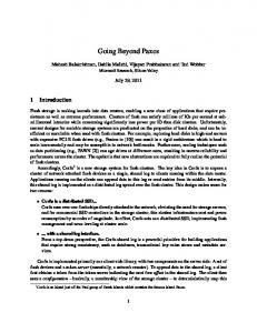
De nition 3.3.2 A distributed system is the composition of process automata modeling some set J of processes and a communication system for J . In this thesis we will always compose automata that model the set of all processes I . Thus we de ne the communication system Scha to be the communication system for the set I of all processes. Figure 3-2 shows this communication system and its interactions with the external environment. Duplicate i,j Send i,j
Receive i,j
Receive j,i
Send j,i CHANNEL i,j
Lose n,n CHANNEL j,i
Receive 1,2
S CHA
CHANNEL n,n
CHANNEL 1,2
CHANNEL 1,1
Send n,n
Send 1,2
Receive n,n
Send 1,1 Receive 1,1
Figure 3-2: The communication system Scha Next we provide the de nition of \stable" execution fragment for a distributed system exploiting the de nitions of stable execution fragment given previously for channels and process automata.
De nition 3.3.3 Given a distributed system S , we say that an execution fragment
� of S is \stable" if:
1. for all automata processi modelling process i, i 2 S it holds that �jprocessi is a stable execution fragment for process i.
45
2. for all channels channeli;j with i; j 2 S it holds that �jchanneli;j is a stable execution fragment for channeli;j .
Finally we provide the de nition of \nice" execution fragment that captures the conditions under which paxos satis es termination.
De nition 3.3.4 Given a distributed system S , we say that an execution fragment
� of S is \nice" if � is a stable execution fragment and a majority of the processes are alive in �.
The above de nition requires a majority of processes to be alive. As will be explained in Chapter 6, the property of majorities needed by the paxos algorithm is that any two majorities have one element on common. Hence any quorum scheme could be used. In the rest of the thesis, we will use the word \system" to mean \distributed system".
46
Chapter 4 The consensus problem Several variations of the consensus problem have been studied. These variations depends on the model used. In this chapter we provide a formal de nition of the consensus problem that we consider.
4.1 Overview In a distributed system processes need to cooperate and fundamental to such cooperation is the problem of reaching agreement on some data upon which the computation depends. Well known practical examples of agreement problems arise in distributed databases, where data managers need to agree on whether to commit or abort a given transaction, and ight control systems, where the airplane control system and the ight surface control system need to agree on whether to continue or abort a landing in progress. In the absence of failures, achieving agreement is a trivial task. An exchange of information and a common rule to make a decision is enough. However the problem becomes much more complex in the presence of failures. Several di�erent but related agreement problems have been considered in the literature. All have in common that processes start the computation with initial values and at the end of the computation each process must reach a decision. The variations mostly concern stronger or weaker requirements that the solution to the 47
problem has to satisfy. The requirement that a solution to the problem has to satisfy are captured by three properties, usually called agreement, validity and termination. As an example, the agreement condition may state that no two processes decide on di�erent values, the validity condition may state that if all the initial values are equal then the (unique) decision must be equal to the initial value and the termination condition may state that every process must decide. A weaker agreement condition may require that only non-faulty processes agree on the decision (this weaker condition is necessary, for example, when considering Byzantine failures for which the behavior of a faulty process is unconstrained). A stronger validity condition may state that every decision must be equal to some initial value. It is clear that the de nition of the consensus problem must take into account the distributed setting in which the problem is considered. About synchrony, several model variations, ranging from the completely asynchronous setting to the completely synchronous one, can be considered. A completely asynchronous model is one with no concept of real time. It is assumed that messages are eventually delivered and processes eventually respond, but it may take arbitrarily long. In a completely synchronous model the computation proceeds in a sequence of steps1 . At each step processes receive messages sent in the previous step, perform some computation and send messages. Steps are taken at regular intervals of time. Thus in a completely synchronous model, processes act as in a single synchronous computer. Between the two extremes of complete synchrony and complete asynchrony, other models with partial synchrony can be considered. These models assume upper bounds on the message transmission time and on the process response time. These upper bounds may be known or unknown to the processes. Moreover processes have some form of real-time clock to take advantage of the time bounds. Failures may concern both communication channels and processes. In synchronous and partially synchronous models, timing failures are considered. Communication failures can result in loss of messages. Duplication and reordering of messages may Usually these steps are called \rounds". However in this thesis we use the word \round" with a di�erent meaning. 1
48
be considered failures, too. Models in which incorrect messages may be delivered are seldom considered since there are many techniques to detect the alteration of a message. The weakest assumption made about process failures is that a faulty process has an unrestricted behavior. Such a failure is called a Byzantine failure. Byzantine failures are often considered with authentication; authentication provides a way to sign messages, so that, even a Byzantine-faulty process cannot send a message with the signature of another process. More restrictive models permit only omission failures, in which a faulty process fails to send some messages. The most restrictive models allow only stopping failures, in which a failed process simply stops and takes no further actions. Some models assume that failed processes can be restarted. Often it is assumed that there is some form of stable storage that is not a�ected by a stopping failure; a stopped process is restarted with its stable storage in the same state as before the failure and with every other part of its state restored to some initial values. In synchronous and partially synchronous models messages are supposed to be delivered and processes are expected to act within some time bounds. A timing failure is a violation of those time bounds. Real distributed systems are often partially synchronous systems subject to process and channel failures. Though timely responses can be provided in real distributed systems, the possibility of process and channels failures makes impossible to guarantee that timing assumptions are always satis ed. Thus real distributed systems su�er timing failures, too. The possibility of timing failures in a partially synchronous distributed system means that the system may as well behave like an asynchronous one. Unfortunately, reaching consensus in asynchronous systems, is impossible, unless it is guaranteed that no failures happen [18]. Henceforth, to solve the problem we need to rely on the timing assumptions. Since timing failures are anyway possible, safety properties, that is, agreement and validity conditions, must not depend at all on timing assumptions. However we can rely on the timing assumptions for the termination condition.
49
4.2 Formal de nition In Section 3 we have described the distributed setting we consider in this thesis. In summary, we consider a partial synchronous system of n processes in a complete network; processes are subject to stop failures and recoveries and have stable storage; channels can lose, duplicate and reorder messages; timing failures are also possible. Next we give a formal de nition of the consensus problem we consider. For each process i there is an external agent that provides an initial value v by means of an action Init(v)i2. We denote by V the set of possible initial values and, given a particular execution �, we denote by V� the subset of V consisting of those values actually used as initial values in �, that is, those values provided by Init(v)i actions executed in �. A process outputs a decision v by executing an action Decide(v)i. If a process i executes action Decide(v)i more than once then the output value v must be the same. To solve the consensus problem means to give a distributed algorithm that, for any execution � of the system, satis es
� Agreement: All the Decide(v) actions in � have the same v. � Validity: For any Decide(v) action in �, v belongs to V�. and, for any admissible execution �, satis es
� Termination: If � = and is a nice execution fragment and for each
process i alive in an Init(v)i action occurs in � when process i is alive, then any process i alive in , executes a Decide(v)i action in �.
The agreement and termination conditions require, as one can expect, that correct processes \agree" on a particular value. The validity condition is needed to relate the output value to the input values (otherwise a trivial solution, i.e. always output a default value, exists). We remark that usually it is assumed that for each process i the Init(v) action is executed at most once; however we do not need this assumption. 2
i
50
4.3 Bibliographic notes paxos solves the consensus problem in a partially synchronous distributed system
achieving termination when the system executes a nice execution fragment. Allowing timing failures, the partially synchronous system may behave as an asynchronous one. A fundamental theoretical result, proved by Fischer, Lynch and Paterson [18] states that in an asynchronous system there is no consensus algorithm even in the presence of only one stopping failure. Essentially the impossibility result stem from the inherent di�culty of determining whether a process has actually stopped or is only slow. The paxos algorithm was devised by Lamport. In the original paper [29], the paxos algorithm is described as the result of discoveries of archaeological studies of an ancient Greek civilization. The paxos algorithm is presented by explaining how the parliament of this ancient Greek civilization worked. A proof of correctness is provided in the appendix of that paper. A time-performance analysis is discussed. Many practical optimizations of the algorithm are also discussed. In [29] there is also presented a variation of paxos that considers multiple concurrent runs of paxos when consensus has to be reached on a sequence of values. We call this variation the multipaxos algorithm. multipaxos can be easily used to implement a data replication algorithm. In [34] a data replication algorithm is provided. It incorporates ideas similar to the ones used in paxos. In the class notes of Principles of Computer Systems [31] taught at MIT, a description of paxos is provided using a speci cation language called SPEC. The presentation in [31] contains the description of how a round of paxos is conducted. The leader election problem is not considered. Timing issues are not considered; for example, the problem of starting new rounds is not addressed. A proof of correctness, written also in SPEC, is provided. Our presentation di�ers from that of [31] in the following aspects: it uses the I/O automata models; it provides all the details of the algorithm; it provides a modular description of the algorithm, including auxiliary 51
parts such as a failure detector module and a leader elector module; along with the proof of correctness, it provides a performance and fault-tolerance analysis. In [32] Lampson provides a brief overview of the paxos algorithm together with the key points for proving the correctness of the algorithm. In [11] three di�erent partially synchronous models are considered. For each of them and for di�erent types of failure an upper bound on the number of failures that can be tolerated is shown, and algorithms that achieve the bounds are given. A model studied in [11] considers a distributed setting similar to the one we consider in this thesis: a partially synchronous distributed system in which upper bounds on the process response time and message delivery time hold eventually; the failures considered are process stop failures (also other models that consider omission failures, Byzantine failures with and without authentication are studied in [11]). The protocol provided in [11], the DLS algorithm for short, needs a linear, in the number of processes, amount of time from the point in which the upper bounds on the process response time and message delivery time start holding. This is similar to the paxos performance which requires a linear amount of time to achieve termination when the system executes a nice execution fragment. However the DLS algorithm does not consider process recoveries and it is resilient to a number of process stopping failures which is less or equal to half the number of processes. This can be related to paxos by the fact that paxos requires a majority of processes alive to reach termination. The paxos algorithm is resilient also to channel failures while the DLS algorithm does not consider channel failures. paxos bears some similarities with the standard three-phase commit protocol:
both require, in each round, an exchange of 5 messages. However the standard commit protocol requires a reliable leader elector while paxos does not. Moreover paxos sends information on the value to agree on only in the third message of a round (while the commit protocol sends it in the rst message) and because of this, multipaxos can exchange the rst two messages only once for many instances and use only the exchange of the last three messages for each individual consensus problem. 52
Chapter 5 Failure detector and leader elector In this chapter we provide a failure detector algorithm and then we use it to implement a leader election algorithm, which in turn will be used in Chapter 6 to implement paxos. The failure detector and the leader elector we implement here are both sloppy, meaning that they are guaranteed to give accurate information on the system only in a stable execution. However, this is enough for implementing paxos.
5.1 A failure detector In this section we provide an automaton that detects process failures and recoveries and we prove that the automaton satis es certain properties that we will need in the rest of the thesis. We do not provide a formal de nition of the failure detection problem, however, roughly speaking, the failure detection problem is the problem of checking which processes are alive and which ones are stopped. Without some knowledge of the passage of time it is not possible to detect failures; thus to implement a failure detector we need to rely on timing assumptions. Figure 5-1 shows a Clock GT automaton, called detector(z; c)i. In our setting failures and recoveries are modeled by means of actions Stopi and Recoveri . These two actions are input actions of detector(z; c)i. Moreover detector(z; c)i has InformStopped(j )i and InformAlive(j )i as output actions which are executed when, respectively, the stopping and the recovering of process j are detected. Automaton detector(z; c)i 53
detector(z; c)i
Signature: Input: Internal: Output: Time-passage:
Receive(m) , Stop , Recover Check(j ) InformStopped(j ) , InformAlive(j ) , Send(m) � (t) j;i
i
i
i
i
i
i;j
State: Clock 2 R Status 2 falive; stoppedg Alive 2 2I for all j 2 I : Prevrec(j ) 2 R�0 Lastinform(j ) 2 R�0 Lastsend(j ) 2 R�0 Lastcheck(j ) 2 R�0
Actions: input Stop
initially arbitrary initially alive initially I initially arbitrary initially Clock initially Clock initially Clock
internal Check(j ) Pre: Status = alive j 2 Alive
i
i
E�: Status := stopped
input Recover
E�: Lastcheck(j ) := Clock + c if Clock > Prevrec(j ) + z + d then Alive := Alive n fj g
i
E�: Status := alive
internal Send(\Alive")
output InformStopped(j ) Pre: Status = alive j 62 Alive
i;j
Pre: Status = alive E�: Lastsend(j ) := Clock + z
input Receive(\Alive")
i
E�: Lastinform(j ) := Clock + `
j;i
E�: if Status = alive then Prevrec(j ) := Clock if j 62 Alive then Alive := Alive [ fj g Lastcheck(j ) := Clock + c
output InformAlive(j ) Pre: Status = alive j 2 Alive
i
E�: Lastinform(j ) := Clock + `
time-passage � (t)
Pre: Status = alive E�: Let t0 be such that 8j; Clock + t0 � Lastinform(j ) 8j; Clock + t0 � Lastsend(j ) 8j; Clock + t0 � Lastcheck(j ) Clock := Clock + t0
Figure 5-1: Automaton detector for process i 54
works by having each process constantly sending \Alive" messages to each other process and checking that such messages are received from other processes. It sends at least one \Alive" message in an interval of clock time of a xed length z (i.e., if an \Alive" message is sent at time t then the next one is sent before time t + z) and checks for incoming messages at least once in an interval of time of a xed length c. Let us denote by Sdet the system consisting of system Scha and an automaton detector(z; c)i for each process i 2 I . Figure 5-2 shows Sdet . InformStopped (j)i
InformAlive (j) i
InformAlive (j)1
InformStopped(j)n InformAlive (j)n
InformStopped (j)1
S DET
DETECTOR i DETECTOR n
DETECTOR 1 Send i,j
Receive j,i Send n,j
Receive j,1
Receive j,n
Send 1,j
S CHA
Figure 5-2: The system Sdet The next two lemmas state that if an execution fragment of system Sdet is stable then after some time the information provide by the failure detector correctly re ects the status of the processes.
Lemma 5.1.1 If an execution fragment � of Sdet, starting in a reachable state and lasting for more than z + c + ` + 2d time, is stable and process i is stopped in �, then by time z + c + ` + 2d, for each process j alive in �, an action InformStopped(i)j is executed and no subsequent InformAlive(i)j action is executed in �.
55
Proof: Let j be any alive process, and let t0 be the Clockj value of process j at
the beginning of �. Notice that, since � is stable, at time � in �, we have that Clockj = t0 + �. Now, notice that channeli;j is a subsystem of Sdet, that is, Sdet is the composition of channeli;j and other automata. By Theorem 2.6.10 the projection �jchanneli;j is an execution fragment of channeli;j and thus any property true for channeli;j in �jchanneli;j is true for Sdet in �; in particular we can use Lemma 3.2.3. Since � is stable and starts in a reachable state we have that �jchanneli;j is stable and starts in a reachable state. Thus by Lemma 3.2.3, any message from i to j that is in the channel at the beginning of � is delivered by time d and consequently, since process i is stopped in �, no message from process i is received by process j after time d. We distinguish two possible cases. Let s be the rst state of � after which no further messages from i are received by j and let �s be the action that brings the system into state s. Notice that the time of occurrence of �s is before or at time d. Case 1: Process i 62 s:Alivej . Then, by the code of detectori an action InformStopped(i)j is executed within ` time after s. Clearly action InformStopped(i)j is executed after s and, since the time of occurrence of �s is � d then it is executed before or at time d + `. Moreover since no messages from i are received after s, no InformAlive(i)j can happen later on. Thus the lemma is proved in this case. Case 2: Process i 2 s:Alivej . Let Prevrec be the value of Clockj at the moment when the last \Alive" message from i is received from j . Since no message from process i is received by process j after s and the time of occurrence of �s is � d, we have that Prevrec � t0 + d; indeed, as we observed before, at time � in �, we have that Clockj = t0 + �, for any �. Since process i is supposed to send a new \Alive" message within z time from the previous one and the message may take up to d time to be delivered, a new \Alive" message from process i is expected by process j before Clockj passes the value Prevrec + z + d. However, no messages are received when Clockj > Prevrec. By the code of detector(z; c)j an action Check(i)j occurs after time Prevrec + z + d and before or at time Prevrec + z + c + d; indeed, a check action occur at least once in an interval of time of length c. When this action occurs, 56
since Clockj > Prevrec + z + d, it removes process i from the Alivej set (see code). Thus by time Prevrec + z + c + d process i is not in Alivej . Since Prevrec � t0 + d, we have that process i is not in Alivej before Clockj passes t0 + z + c + 2d. Action InformStopped(i)j is executed within additional ` time, that is before Clockj passes t0 + z + c + 2d + `. Notice also|and we will need this for the second part of the proof|that this action happens when Clockj > t0 + z + c + 2d > t0 + d. Thus we have that action InformStopped(i)j is executed by time z + c + 2d + `. Since we are considering the case when process i is in Alivej at time d, action InformStopped(i)j is executed after time d. This is true for any alive process j . Thus the lemma is proved also in this case. This concludes the proof of the rst part of the lemma. Now, since no messages from i are received by j after time d, that is, no message from i to j is received when Clockj > t0 + d and, by the rst part of this proof, InformStopped(i)j happens when Clockj > t0 + d, we have that no InformAlive(i)j action can occur after InformStopped(i)j has occurred. This is true for any alive process j . Thus also the second part of the lemma is proved.
Lemma 5.1.2 If an execution fragment � of Sdet, starting in a reachable state and
lasting for more than z + d + ` time, is stable and process i is alive in �, then by time z + d + `, for each process j alive in �, an action InformAlive(i)j is executed and no subsequent InformStopped(i)j action is executed in �.
Proof: Let j be any alive process, and let t0 be the value of Clocki and t00 be the value
of Clockj at the beginning of �. Notice that, since � is stable, at time � in �, we have that Clocki = t0 +� and Clockj = t00 +�. Now, notice that channeli;j is a subsystem of Sdet, that is, Sdet can be though of as the composition of channeli;j and other automata. By Theorem 2.6.10 �jchanneli;j is an execution of channeli;j and thus any property of channeli;j true in �jchanneli;j is true for Sdet in �; in particular we can use Lemma 3.2.3. Since process i is alive in � and � is stable, process i sends an \Alive" message to process j by time z and, by Lemma 3.2.3, such a message is received by process j by time z + d. Whence, before Clockj passes t00 + z + d, action 57
Receive(\Alive")i;j is executed and thus process i is put into Alivej (unless it was already there). Once process i is into Alivej , within additional ` time, that is before Clockj passes t00 + z + d + `, or equivalently, by time z + d + `, action InformAlive(i)j is executed. This is true for any process j . This proves the rst part of the Lemma. Let t be the time of occurrence of the rst Receive(\Alive")i;j executed in �; by the rst part of this lemma, t � z + d. Then since � is stable, process i sends at least one \Alive" message in an interval of time z and each message takes at most d to be delivered. Thus in any interval of time z + d process j executes a Receive(\Alive")i;j . This implies that the Clockj variable of process j never assumes values greater than Prevrec(i)j + z + d, which in turns imply that every Check(i)j action does not remove process i from Alivej . Notice that process i may be removed from Alivej before time t. However it is put into Alivej at time t and it is not removed later on. Thus also the second part of the lemma is proved. The strategy used by detector(z; c)i is a straightforward one. For this reason it is very easy to implement. However the failure detector so obtained is not reliable, i.e., it does not give accurate information, in the presence of failures (Stopi, Losei;j , irregular executions). For example, it may consider a process stopped just because the \Alive" message of that process was lost in the channel. Automaton detector(z; c)i is guaranteed to provide accurate information on faulty and alive processes only when the system is stable. In the rest of this thesis we assume that z = ` and c = `, that is, we use detector(`; `)i . This particular strategy consists of sending an \Alive" message in each interval of ` time (i.e., we assume z = `) and of checking for incoming messages at least once in each interval of ` time (i.e., we assume c = `). In practice the choice of z and c may be di�erent. However for the sake of simplicity we get rid of parameters z and c by assuming z = ` and c = `. Lemmas 5.1.3 and 5.1.4 can be restated as follows.
Lemma 5.1.3 If an execution fragment � of Sdet, starting in a reachable state and lasting for more than 3` + 2d time, is stable and process i is stopped in �, then by
58
time 3` + 2d, for each process j alive in �, an action InformStopped(i)j is executed and no subsequent InformAlive(i)j action is executed in �.
Lemma 5.1.4 If an execution fragment � of Sdet, starting in a reachable state and lasting for more than d + 2` time, is stable and process i is alive in �, then by time d + 2`, for each process j alive in �, an action InformAlive(i)j is executed and no subsequent InformStopped(i)j action is executed in �.
5.2 A leader elector Electing a leader in an asynchronous distributed system is a di�cult task. An informal argument that explains this di�culty is that the leader election problem is somewhat similar to the consensus problem, which, in an asynchronous system subject to failures is unsolvable [18], in the sense that to elect a leader all processes must reach consensus on which one is the leader. As for the failure detector, we need to rely on timing assumptions. It is fairly clear how a failure detector can be used to elect a leader. Indeed the failure detector gives information on which processes are alive and which ones are not alive. This information can be used to elect the current leader. We use the detector(`; `)i automaton to check for the set of alive processes. Figure 5-3 shows automaton leaderelectori which is an MMT automaton. Remember that we use MMT automata to describe in a simpler way some Clock GT automata. Automaton leaderelectori interacts with detector(`; `)i by means of actions InformStopped(j )i, which inform process i that process j has stopped, and InformAlive(j )i, which inform process i that process j has recovered. Each process updates its view of the set of alive processes when these two actions are executed. The process with the biggest identi er in the set of alive processes is declared leader. We denote with Slea the system consisting of Sdet composed with a leaderelectori automaton for each process i 2 I . Figure 5-4 shows Slea. Since detector(`; `)i is not a reliable failure detector, also leaderelectori is not reliable. Thus, it is possible that processes have di�erent views of the system so that more than one process considers itself leader, or the process supposed to be the 59
leaderelectori
Signature: InformStopped(j ) , InformAlive(j ) , Stop , Recover Leader , NotLeader
Input: Output:
i
i
i
i
i
i
State: Status 2 falive; stoppedg Pool 2 2I
initially alive initially fig
Derived variable: Leader, de ned as max of Pool
Actions: input Stop
input Recover
i
E�: Status := stopped
output Leader
i
E�: Status := alive
output NotLeader Pre: Status = alive i= 6 Leader
i
i
Pre: Status = alive i = Leader E�: none
E�: none
input InformStopped(j ) E�: if Status = alive then Pool := Pool n fj g
input InformAlive(j )
i
i
E�: if Status = alive Pool := Pool [ fj g
Tasks and bounds: fLeader , NotLeader g, bounds [0; `] i
i
Figure 5-3: Automaton leaderelector for process i
60
Leader i
NotLeader i
NotLeader 1
Leader n NotLeader n
Leader 1
S LEA LEADERELECTOR i
LEADERELECTOR1
LEADERELECTOR n
InformStopped (j)
S DET
InformAlive (j) i
i
DETECTOR i DETECTOR n
DETECTOR 1 Send i,j Receive
Receive
j,i
Send n,j j,1
Receive j,n
Send 1,j
S CHA
Figure 5-4: The system Slea leader is actually stopped. However as the failure detector becomes reliable when the system Sdet executes a stable execution fragment (see Lemmas 5.1.3 and 5.1.4), also the leader elector becomes reliable when system Slea is stable. Notice that when Slea executes a stable execution fragment, so does Sdet. Formally we consider a process i to be leader if Leaderi = i. That is, a process i is leader if it consider itself to be the leader. This allows multiple or no leaders and does not require other processes to be aware of the leader or the leaders. The following de nitions give a much more precise notion of leader.
De nition 5.2.1 A state s of system Slea, is a \unique-leader" state if there exists
an alive process i such that for all alive processes j it holds that s:Leaderj = i. Process i is the \leader" in state s.
De nition 5.2.2 An execution � of system Slea, is a \unique-leader" execution if 61
all the states of � are unique-leader states with the same leader in all the states.
The next lemma states that in a stable execution fragment, eventually there will be a unique-leader state.
Lemma 5.2.3 If an execution fragment � of Slea, starting in a reachable state and lasting for more than 4` +2d, is stable, then by time 4` +2d, there is a state occurrence s such that state s and all the states after s are unique-leader states. Moreover the unique leader is always the process with the biggest identi er among the processes alive in �.
Proof: First notice that the system Slea consists of system Sdet composed with
other automata. Hence by Theorem 2.6.10 we can use any property of Sdet. In particular we can use Lemmas 5.1.3 and 5.1.4 and thus we have that by time 3` + 2d each process has a consistent view of the set of alive and stopped processes. Let i be the leader. Since � is stable and thus also regular, by Lemma 2.5.4, within additional ` time, actions Leaderj and NotLeaderj are consistently executed for each process j , including process j = i. The fact that i is the the process with the biggest identi er among the processes alive in � follows directly from the code of leaderelectori.
We remark that, for many algorithms that rely on the concept of leader, it is important to provide exactly one leader. For example when the leader election is used to generate a new token in a token ring network, it is important that there is exactly one process (the leader) that generates the new token, because the network gives the right to send messages to the owner of the token and two tokens may result in an interference between two communications. For these algorithms, having two or more leaders jeopardizes the correctness. Hence the sloppy leader elector provided before is not suitable. However for the purpose of this thesis, leaderelectori is all we need.
62
5.3 Bibliographic notes In an asynchronous system it is impossible to distinguish a very slow process from a stopped one. This is why the consensus problem cannot be solved even in the case where at most one process fails [18]. If a reliable failure detector were provided then the consensus problem would be solvable. This clearly implies that in a completely asynchronous setting no reliable failure detector can be provided. Chandra and Toueg [5] gave a de nition of unreliable failure detector, and characterized failure detectors in terms of two properties: completeness, which requires that the failure detector eventually suspect any stopped process, and accuracy, which restricts the mistakes a failure detector can make. No failure detectors are actually implemented in [5]. The failure detector provided in this thesis di�ers from those classi ed by Chandra and Toueg in that it provides reliability conditional to the system stabilization. If the system eventually stabilizes then our failure detector can be classi ed in the class of the eventually perfect failure detectors. However it should be noted that in order to achieve termination we actually do not need that the system become stable forever but only for a su�ciently long time. Chandra, Hadzilacos and Toueg [4] identi ed the \weakest" failure detector that can be used to solve the consensus problem. Failure detectors have practical relevance since it is often important to establish which processes are alive and which ones are stopped. The need for a leader in a distributed computation arises in many practical situations, like, for example, in a token ring network. However in asynchronous systems there is the inherent di�culty of distinguishing a stopped process from a slow one.
63
Chapter 6 The paxos algorithm paxos was devised a very long time ago1 but its discovery, due to Lamport, is very
recent [29]. In this chapter we describe the paxos algorithm, provide an implementation using Clock GT automata, prove its correctness and analyze its performance. The performance analysis is given assuming that there are no failures nor recoveries, and a majority of the processes are alive for a su�ciently long time. We remark that when no restrictions are imposed on the possible failures, the algorithm might not terminate.
6.1 Overview Our description of paxos is modular: we have separated various parts of the overall algorithm; each piece copes with a particular aspect of the problem. This approach should make the understanding of the algorithm much easier. The core part of the algorithm is a module that we call basicpaxos; this piece incorporates the basic ideas on which the algorithm itself is built. The description of this piece is further subdivided into three components, namely bpleader, bpagent and bpsuccess. In basicpaxos processes try to reach a decision by running what we call a \round". A process starting a round is the leader of that round. basicpaxos guar1
The most accurate information dates it back to the beginning of this millennium [29].
64
antees that, no matter how many leaders start rounds, agreement and validity are not violated. However to have a complete algorithm that satis es termination when there are no failures for a su�ciently long time, we need to augment basicpaxos with another module; we call this module starteralg. The functionality of starteralg is to make the current leader start a new round if the previous one is not completed within some time bound. Leaders are elected by using the leaderelector algorithm provided in Chapter 5. We remark that this is possible because the presence of two or more leaders does not jeopardize agreement or validity; however, to get termination there must be a unique leader. Thus, our implementation of paxos is obtained by composing the following automata: channeli;j for the communication between processes, detectori and leaderelectori for the leader election, basicpaxosi and starteralgi , for every process i; j 2 I . The resulting system is called Spax. Figure 6-1 shows the automaton at process i. Notice that not all of the actions are drawn in the picture: we have drawn only some of them and we refer to the formal code for all of the actions. Actions Stopi and Recoveri are input actions of all the automata. The Spax automaton at process i interacts with automata at other processes by sending messages over the channels. Channels are not drawn in the picture. Figure 6-2 shows the messages exchanged by processes i and j . The automata that send and receive these messages are shown in the picture. We remark that channels and actions interacting with channels are not drawn, as well as other actions for the interaction with other automata. It is worth to remark that some pieces of the algorithm do need to be able to measure the passage of the time (detectori, starteralgi and bpsuccessi) while others do not. We will prove (Theorems 6.2.15 and 6.2.18) that the system Spax solves the consensus problem ensuring partial correctness|any output is guaranteed to be correct, that is, agreement and validity are satis ed|and (Theorem 6.4.2) that Spax guar65
DETECTOR i
Stop i
InformRecovered (j) i
InformStopped (j) i
Recover i LEADERELECTOR i
Leader i
NotLeader i
STARTERALG i Init (v) i
NewRound i
RndSuccess i
BPLEADER i BPAGENT i
RndSuccess i BASICPAXOS i
Decide (v) i
BPSUCCESS i
Figure 6-1: paxos: process i.
(r,‘‘Collect’’) (r,‘‘Last’’,r’,v) BPAGENTj
(r,‘‘Begin’’,v)
BPLEADER i
(r,‘‘Accept’’)
RndSuccess (v) i
(‘‘Success’’,v) BPSUCCESS i
BPSUCCESS j (‘‘Ack’’)
Figure 6-2: basicpaxos: Messages. 66
antees also termination when the system executes a nice execution fragment, that is, without failures and recoveries and with at least a majority of the processes remaining alive.
Roadmap for the rest of the chapter. In Section 6.2 we provide automaton
basicpaxos. This automaton is responsible for carrying out a round in response to
an external request. We prove that any round satis es agreement and validity and we provide a performance analysis for a successful round. Then in Section 6.3 we provide automaton starteralg which takes care of the problem of starting new rounds. In Section 6.4 we prove that the entire system Spax is correct and provide a performance analysis. In Section 6.5 we provide some comments about the number of messages used by the algorithm. Finally Section 6.6 contains some concluding remarks.
6.2 Automaton basicpaxos In this section we present the automaton basicpaxos which is the core part of the paxos algorithm. We begin by providing an overview of how automaton basicpaxos works, then we provide the automaton code along with a detailed description and nally we prove that it satis es agreement and validity.
6.2.1 Overview The basic idea is to have processes propose values until one of them is accepted by a majority of the processes; that value is the nal output value. Any process may propose a value by initiating a round for that value. The process initiating a round is said to be the leader of that round while all processes, including the leader itself, are said to be agents for that round. Informally, the steps for a round are the following. 1. To initiate a round, the leader sends a \Collect" message to all agents2 announcing that it wants to start a new round and at the same time asking for 2 Thus it sends a message also to itself. This helps in that we do not have to specify di�erent behaviors for a process according to the fact that it is both leader and agent or just an agent. We just need to specify the leader behavior and the agent behavior.
67
information about previous rounds in which agents may have been involved. 2. An agent that receives a message sent in step 1 from the leader of the round, responds with a \Last" message giving its own information about rounds previously conducted. With this, the agent makes a kind of commitment for this particular round that may prevent it from accepting (in step 4) the value proposed in some other round. If the agent is already committed for a round with a bigger round number then it informs the leader of its commitment with an \OldRound" message. 3. Once the leader has gathered information about previous rounds from a majority of agents, it decides, according to some rules, the value to propose for its round and sends to all agents a \Begin" message announcing the value and asking them to accept it. In order for the leader to be able to choose a value for the round it is necessary that initial values be provided. If no initial value is provided, the leader must wait for an initial value before proceeding with step 3. The set of processes from which the leader gathers information is called the info-quorum of the round. 4. An agent that receives a message from the leader of the round sent in step 3, responds with an \Accept" message by accepting the value proposed in the current round, unless it is committed for a later round and thus must reject the value proposed in the current round. In the latter case the agent sends an \OldRound" message to the leader indicating the round for which it is committed. 5. If the leader gets \Accept" messages from a majority of agents, then the leader sets its own output value to the value proposed in the round. At this point the round is successful. The set of agents that accept the value proposed by the leader is called the accepting-quorum. Since a successful round implies that the leader of the round reached a decision, after a successful round the leader still needs to do something, namely to broadcast the reached decision. Thus, once the leader has made a decision it broadcasts a 68
\Success" message announcing the value for which it has decided. An agent that receives a \Success" message from the leader makes its decision choosing the value of the successful round. We use also an \Ack" message sent from the agent to the leader, so that the leader can make sure that everyone knows the outcome. Voter
Leader
Voter
Leader (r,‘‘Collect’’)
(r,‘‘Collect’’)
(r,‘‘Last’’,r’,v)
(r,‘‘OldRound’’,r’)
(r,‘‘Begin’’,v)
(r,‘‘Begin’’,v)
(r,‘‘Accept’’)
(r,‘‘OldRound’’,r’)
(a)
(b)
Voter
Leader (‘‘Success’’,v)
(‘‘Ack’’)
(c)
Figure 6-3: Exchange of messages Figure 6-3 shows: (a) the steps of a successful round r; (b) the responses from an agent that informs the leader that an higher numbered round r0 has been already initiated; (c) the broadcast of a decision. The parameters used in the messages will be explained later. Section 6.2.2 contains a description of the messages. Since di�erent rounds may be carried out concurrently (several processes may concurrently initiate rounds), we need to distinguish them. Every round has a unique 69
identi er. Next we formally de ne these round identi ers. A round number is a pair (x; i) where x is a nonnegative integer and i is a process identi er. The set of round numbers is denoted by R. A total order on elements of R is de ned by (x; i) < (y; j ) i� x < y or, x = y and i < j .
De nition 6.2.1 Round r \precedes" round r0 if r < r0. If round r precedes round r0 then we also say that r is a previous round, with respect to round r0. We remark that the ordering of rounds is not related to the actual time the rounds are conducted. It is possible that a round r0 is started at some point in time and a previous round r, that is, one with r < r0, is started later on. For each process i, we de ne a \+i" operation that given a round number (x; j ) and an integer y, returns the round number (x; j ) +i y = (x + y; i). Every round in the algorithm is tagged with a unique round number. Every message sent by the leader or by an agent for a round (with round number) r 2 R, carries the round number r so that no confusion among messages belonging to di�erent rounds is possible. However the most important issue is about the values that leaders propose for their rounds. Indeed, since the value of a successful round is the output value of some processes, we must guarantee that the values of successful rounds are all equal in order to satisfy the agreement condition of the consensus problem. This is the tricky part of the algorithm and basically all the di�culties derive from solving this problem. Consistency is guaranteed by choosing the values of new rounds exploiting the information about previous rounds from at least a majority of the agents so that, for any two rounds, there is at least one process that participated in both rounds. In more detail, the leader of a round chooses the value for the round in the following way. In step 1, the leader asks for information and in step 2 an agent responds with the number of the latest round in which it accepted the value and with the accepted value or with round number (0; j ) and nil if the agent has not yet accepted a value. Once the leader gets such information from a majority of the agents (which is the info-quorum of the round), it chooses the value for its round to be equal to the value 70
of the latest round among all those it has heard from the agents in the info-quorum or equal to its initial value if all agents in the info-quorum were not involved in any previous round. Moreover, in order to keep consistency, if an agent tells the leader of a round r that the last round in which it accepted a value is round r0, r0 < r, then implicitly the agent commits itself not to accept any value proposed in any other round r00, r0 < r00 < r. Given the above setting, if r0 is the round from which the leader of round r gets the value for its round, then, when a value for round r has been chosen, any round r00, r0 < r00 < r, cannot be successful; indeed at least a majority of the processes are committed for round r, which implies that at least a majority of the processes are rejecting round r00 . This, along with the fact that info-quorums and acceptingquorums are majorities, implies that if a round r is successful, then any round with a bigger round number r~ > r is for the same value. Indeed the information sent by processes in the info-quorum of round r~ is used to choose the value for the round, but since info-quorums and accepting-quorums share at least one process, at least one of the processes in the info-quorum of round r0 is also in the accepting-quorum of round r. Indeed, since the round is successful, the accepting-quorum is a majority. This implies that the value of any round r~ > r must be equal to the value of round r, which, in turn, implies agreement. We remark that instead of majorities for info-quorums and accepting-quorums, any quorum system can be used. Indeed the only property that is required is that there be a process in the intersection of any info-quorum with any accepting-quorum.
Example. Figure 6-4 shows how the value of a round is chosen. In this example we have a network of 5 processes, A; B; C; D; E (where the ordering is the alphabetical one) and vA ; vB denote the initial values of A and B . At some point process B is the leader and starts round (1; B ). It receives information from A; B; E (the set fA; B; E g is the infoquorum of this round). Since none of them has been involved in a previous round, process B is free to choose its initial value vB as the value of the round. However it receives acceptance only from B; C (the set fB; C g is the accepting-quorum for this round). Later, process A becomes the leader and starts round (2; A). The info-quorum for this round is fA; D; E g.
71
Round number
Value
(1,B)
vB
(2,A)
vA
(2,D)
vB
(3,A)
vA
(3,B)
vB
A
B
C
D
E
Figure 6-4: Choosing the values of rounds. Empty boxes denote that the process is in the info-quorum, and black boxes denote acceptance. Dotted lines indicate commitments. Since none of this processes has accepted a value in a previous round, A is free to choose its initial value for its round. For round (2; D) the info-quorum is fC; D; E g. This time in the quorum there is process C that has accepted a value in round (1; B ) so the value of this round must be the same of that of round (1; B ). For round (3; A) the info-quorum is fA; B; Eg and since A has accepted the value of round (2; A) then the value of round (2; A) is chosen for round (3; A). For round (3; B ) the info-quorum is fA; C; Dg. In this case there are three processes that accepted values in previous rounds: process A that has accepted the value of round (2; A) and processes C; D, that have accepted the value of round (2; D). Since round (2; D) is the higher round number, the value for round (3; B ) is taken from round (2; D). Round (3; B ) is successful.
To end up with a decision value, rounds must be started until at least one is successful. The basic consensus module basicpaxos guarantees that a new round does not violate agreement or validity, that is, the value of a new round is chosen in 72
such a way that if the round is successful, it does not violate agreement and validity. However, it is necessary to make basicpaxos start rounds until one is successful. We deal with this problem in Section 6.3.
6.2.2 The code In order to describe automaton basicpaxosi for process i we provide three automata. One is called bpleaderi and models the \leader" behavior of the process; another one is called bpagenti and models the \agent" behavior of the process; the third one is called bpsuccessi and it simply takes care of broadcasting a reached decision. Automaton basicpaxosi is the composition of bpleaderi, bpagenti and bpsuccessi. Figures 6-5 and 6-6 show the code for bpleaderi, while Figure 6-7 shows the code for bpagenti. We remark that these code fragments are written using the MMTA model. Remember that we use MMTA to describe in a simpler way Clock GT automata. In section 2.3 we have described a standard technique to transform any MMTA into a Clock GTA. Figures 6-8 and 6-9 show automaton bpsuccessi. The purpose of this automaton is simply to broadcast the decision once it has been reached by the leader of a round. Figures 6-2 and 6-3 describe the exchange of messages used in a round. It is worth noticing that the code fragments are \tuned" to work e�ciently when there are no failures. Indeed messages for a given round are sent only once, that is, no attempt is made to try to cope with losses of messages and responses are expected to be received within given time bounds. Other strategies to try to conduct a successful round even in the presence of some failures could be used. For example, messages could be sent more than once to cope with the loss of some messages or a leader could wait more than the minimum required time before abandoning the current round and starting a new one|this is actually dealt with in Section 6.3. We have chosen to send only one message for each step of the round: if the execution is nice, one message is enough to conduct a successful round. Once a decision has been made, there is nothing to do but try to send it to others. Thus once the decision has been made 73
bpleaderi
Signature:
Input: Receive(m) , m 2 f\Last", \Accept",\OldRound"g Init(v) , NewRound , Stop , Recover , Leader , NotLeader Internal: Collect , BeginCast , GatherLast(m) , m is a \Last" message GatherAccept(m) , m is a \Accept" message GatherOldRound(m) m is a \OldRound" message Output: Send(m) , m 2 f\Collect", \Begin"g Gathered(v) , Continue , RndSuccess(v) j;i
i
i
i
i
i
i
i
i
i
i
i
i;j
i
i
i
State:
Status 2 falive,stoppedg initially alive IamLeader, a boolean initially false Mode 2 fcollect,gatherlast,
CurRnd 2 R HighestRnd 2 R Value 2 V [ fnilg ValFrom 2 R InfoQuo 2 2I AcceptQuo 2 2I InMsgs, multiset of msgs OutMsgs, multiset of msgs
wait, begincast, gatheraccept, decided,done initially done nil initially nil nil initially nil
g
InitValue 2 V [ Decision 2 V [ f
g
initially (0; i) initially (0; i) initially nil initially (0; i) initially fg initially fg initially fg initially fg
Derived Variable:
LeaderAlive, a boolean, true i� Status = alive and IamLeader = true
Actions: input Stop
input Recover
i
input Leader
i
E�: Status := alive
E�: Status := stopped
input NotLeader
i
i
E�: if Status = alive then IamLeader := false
E�: if Status = alive then IamLeader := true
input Receive(m)
output Send(m) Pre: Status = alive m 2 OutMsgs i;j
j;i
E�: if Status = alive then add m to InMsgs j;i
i;j
E�: remove m from OutMsgs i;j
input Init(v)
i
E�: if Status = alive then InitValue := v
Figure 6-5: Automaton bpleader for process i (part 1)
74
Actions: input NewRound
internal Continue
i
E�: if LeaderAlive = true then CurRnd := HighestRnd + 1 HighestRnd := CurRnd Mode := collect i
output Collect
i
Pre: LeaderAlive = true Mode = collect E�: ValFrom := (0; i) InfoQuo := fg AcceptQuo := fg 8j put hCurRnd; \Collect"i in OutMsgs Mode := gatherlast
internal GatherLast(m)
i
Pre: LeaderAlive = true Mode = wait Value = nil InitValue = 6 nil E�: Value := InitValue Mode := begincast
internal BeginCast
i
Pre: LeaderAlive = true Mode = begincast E�: 8j put hCurRnd; \Begin"; Valuei in OutMsgs Mode := gatheraccept
i;j
internal GatherAccept(m)
i
Pre: LeaderAlive = true Mode = gatheraccept m = hr; \Accept"i 2 InMsgs CurRnd = r E�: remove m from InMsgs AcceptQuo := AcceptQuo [fj g if jAcceptQuoj > n=2 then Decision := Value Mode := decided
i
Pre: LeaderAlive = true Mode = gatherlast m = hr; \Last"; r0 ; vi 2 InMsgs CurRnd = r E�: remove m from InMsgs InfoQuo := InfoQuo [ fj g if ValFrom < r0 and v 6= nil then Value := v ValFrom := r0 if jInfoQuoj > n=2 then Mode := gathered
j;i
j;i
output RndSuccess(Decision) Pre: LeaderAlive = true Mode = decided E�: Mode := done
output Gathered(Value)
Pre: LeaderAlive = true Mode = gathered E�: if Value = nil and InitValue 6= nil then Value := InitValue if Value 6= nil then Mode := begincast else Mode := wait
i
internal GatherOldRound(m) Pre: Status = alive m = hr; \OldRound"; r0 i 2 InMsgs i
HighestRnd < r0 E�: remove m from InMsgs HighestRnd := r0
j;i
Tasks and bounds: fCollect , Gathered(v) , Continue , BeginCast , RndSuccess(v) g, bounds [0; `] fGatherLast(m) , m 2 InMsgs, m is a \Last" messageg, bounds [0; `] fGatherAccept(m) , m 2 InMsgs, m is a \Accept" messageg, bounds [0; `] fGatherOldRound(m) , m 2 InMsgs, m is a \OldRound" messageg, bounds [0; `] fSend(m) , m 2 OutMsgsg, bounds [0; `] i
i
i
i
i
i
i
i
i;j
i;j
i;j
Figure 6-6: Automaton bpleader for process i (part 2) 75
bpagenti
Signature:
Input: Receive(m) , m 2 f\Collect", \Begin"g Init(v) , Stop , Recover Internal: LastAccept(m) , m is a \Collect" message Accept(m) , m is a \Begin" message Output: Send(m) , m 2 f"Last", \Accept", \OldRound"g j;i
i
i
i
i
i
i;j
State:
Status 2 falive,stoppedg initially alive LastR 2 R initially (0; i) LastV 2 V [ fnilg initially nil
Actions: input Stop
Commit 2 R initially (0; i) InMsgs, multiset of msgs initially fg OutMsgs, multiset of msgs initially fg
input Recover
i
E�: Status := stopped
i
E�: Status := alive
output Send(m) Pre: Status = alive m 2 OutMsgs
input Receive(m)
i;j
j;i
E�: if Status = alive then add m to InMsgs j;i
E�: remove m from OutMsgs i;j
internal Accept(m) Pre: Status = alive m = hr; \Begin"; vi 2 InMsgs E�: remove m from InMsgs if r � Commit then put hr; \Accept"i in InMsgs
internal LastAccept(m) Pre: Status = alive m = hr; \Collect"i 2 InMsgs E�: remove m from InMsgs if r � Commit then Commit := r put hr; \Last"; LastR; LastVi
i
i
j;i
j;i
i;j
LastR := r, LastV := v else put hr; \OldRound"; Commiti in OutMsgs
i;j
in OutMsgs else put hr; \OldRound"; Commiti in OutMsgs
i;j
input Init(v)
i
E�: if Status = alive then if LastV = nil then LastV := v
Tasks and bounds: fLastAccept(m) , m 2 InMsgs, m is a \Collect" messageg, bounds [0; `] fAccept(m) , m 2 InMsgs, m is a \Begin" messageg, bounds [0; `] fSend(m) , m 2 OutMsgs g, bounds [0; `] i
i
i;j
i;j
i;j
Figure 6-7: Automaton bpagent for process i
76
bpsuccessi
Signature:
Receive(m) , m 2 f\Ack", \Success"g Stop , Recover , Leader , NotLeader , RndSuccess(v) Internal: SendSuccess , Check Output: Send(m) , m 2 f\Ack", \Success"g Decide(v) Time-passage: � (t) Input:
j;i
i
i
i
i
i
i
i
i;j i
State: Clock 2 R Status 2 falive; stoppedg IamLeader, a boolean Decision 2 V [ fnilg Prevsend 2 R [ fnilg LastCheck 2 R [ f1g LastSS 2 R [ f1g For each j 2 I Acked(j ), a boolean LastSendAck(j ) 2 R [ f1g LastSendSuc(j ) 2 R [ f1g OutAckMsgs(j ), set of msgs OutSucMsgs(j ), set of msgs
Actions: input Stop
initially arbitrary initially alive initially false initially nil initially nil initially 1 initially 1 initially false initially 1 initially 1 initially fg initially fg
input Recover
i
input Leader
i
E�: Status := alive
E�: Status := stopped
input NotLeader
i
i
E�: if Status = alive then IamLeader := false LastSS := 1 LastCheck := 1 For each j 2 I LastSendSuc(j ) := 1
E�: if Status = alive and IamLeader = false then IamLeader := true if Decision 6= nil then LastSS := clock + ` PrevSend := nil
input Receive(h\Ack"i)
output Send(m) Pre: Status = alive m 2 OutAckMsgs(j ) E�: OutAckMsgs(j ) := fg LastSendAck(j ) := 1 i;j
j;i
E�: if Status = alive then Acked(j ) := true
i;j
input Receive(h\Success",vi)
j;i
E�: if Status = alive then Decision := v put h\Ack"i into OutAckMsgs(j ) LastSendAck(j ) := Clock + `
output Send(m) Pre: Status = alive m 2 OutSucMsgs(j ) E�: OutSucMsgs(j ) := fg LastSendSuc(j ) := 1 i;j
i;j
i;j
Figure 6-8: Automaton bpsuccess for process i (part 1) 77
input RndSuccess(v)
internal Check
i
E�: if Status = alive then Decision := v if IamLeader = true then LastSS := Clock + ` PrevSend := nil
internal SendSuccess
i
Pre: Status = alive PrevSend 6= nil Clock > PrevSend + (2` + 2d) E�: PrevSend := nil LastSS := Clock + ` LastCheck := 1
output Decide(v) Pre: Status = alive Decision = 6 nil
i
Pre: Status = alive IamLeader = true Decision = 6 nil PrevSend = nil 9j 6= i, Acked(j ) = false E�: 8j 6= i such that Acked(j ) = false put h\Success",Decisioni in OutSucMsgs(j ) LastSendSuc(j ) := Clock + ` PrevSend := Clock LastCheck := Clock + (2` + 2d) + ` LastSS := 1
i
Decision = v E�: none
time-passage � (t)
i;j
Pre: Status = alive E�: Let t0 be such that Clock+t0 � LastCheck Clock+t0 � LastSS and for each j 2 I Clock+t0 � LastSendAck(j ) Clock+t0 � LastSendSuc(j ) Clock := Clock+t0
Figure 6-9: Automaton bpsuccess for process i (part 2) by the leader, the leader repeatedly sends the decision to the agents until it gets an acknowledgment. We remark that also in this case, in practice, it is important to choose appropriate time-outs for the re-sending of a message; in our implementation we have chosen to wait the minimum amount of time required by an agent to respond to a message from the leader; if the execution is stable this is enough to ensure that only one message announcing the decision is sent to each agent. We remark that there is some redundancy that derives from having separate automata for the leader behavior and for the broadcasting of the decision. For example, both automata bpleaderi and bpsuccessi need to be aware of the decision, thus both have a Decision variable (the Decision variable of bpsuccessi is updated when action RndSuccessi is executed by bpleaderi after the Decision variable of bpleaderi is set). Having only one automaton would have eliminated the need of such a duplication. However we preferred to separate bpleaderi and bpsuccessi because they accomplish di�erent tasks. In addition to the code fragments of bpleaderi, bpagenti and bpsuccessi, we 78
provide here some comments about the messages, the state variables and the actions.
Messages. In this paragraph we describe the messages used for communication
between the leader i and the agents of a round. Every message m is a tuple of elements. The messages are:
1. \Collect" messages, m =hr;\Collect"ii;j . This message is sent by the leader of a round to announce that a new round, with number r, has been started and at the same time to ask for information about previous rounds. 2. \Last" messages, m =hr,\Last",r0,vij;i. This message is sent by an agent to respond to a \Collect" message from the leader. It provides the last round r0 in which the agent has accepted a value, and the value v proposed in that round. If the agent did not accept any value in previous rounds, then v is either nil or the initial value of the agent and r0 is (0; j ). 3. \Begin" messages, m = hr;\Begin",vii;j . This message is sent by the leader of round r to announce the value v of the round and at the same time to ask to accept it. 4. \Accept" messages, m = hr; \Accept"ij;i. This message is sent by an agent to respond to a \Begin" message from the leader. With this message an agent accepts the value proposed in the current round. 5. \OldRound" messages, m = hr; \OldRound"; r0ij;i. This message is sent by an agent to respond either to a \Collect" or a \Begin" message. It is sent when the agent is committed to reject round r and it informs the leader about round r0, which is the higher numbered round for which the agent is committed to reject round r. 6. \Success" messages, m = h\Success",vii;j . This message is sent by the leader to broadcast the decision. 7. \Ack" messages, m =h\Ack"ij;i. This message is an acknowledgment, so that the leader can be sure that an agent has received the \Success" message. 79
We use the kind of a message to indicate any message of that kind. For example the notation m 2 f\Collect", \Begin"g means that m is either a \Collect" message, that is m =hr,"Collect"i for some r, or a \Begin" message, that is m =hr,"Begin",vi for some r and v.
Automaton
bpleaderi . Variable Statusi is used to model process failures and
recoveries. Variable IamLeaderi keeps track of whether the process is leader. Variable Modei is used like a program counter, to go through the steps of a round. Variable InitValuei contains the initial value of the process. Variable Decisioni contains the value, if any, decided by process i. Variable CurRndi contains the number of the round for which process i is currently the leader. Variable HighestRndi stores the highest round number seen by process i. Variable Valuei contains the value being proposed in the current round. Variable ValFromi is the round number of the round from which Valuei has been chosen (recall that a leader sets the value for its round to be equal to the value of a particular previous round, which is round ValFromi). Variable InfoQuoi contains the set of processes for which a \Last" message has been received by process i (that is, the info-quorum). Variable AcceptQuo contains the set of processes for which an \Accept" message has been received by process i (that is, the accepting-quorum). We remark that in the original paper by Lamport, there is only one quorum which is xed in the rst exchange of messages between the leader and the agents, so that only processes in that quorum can accept the value being proposed. However, there is no need to restrict the set of processes that can accept the proposed value to the info-quorum of the round. Messages from processes in the info-quorum are used only to choose a consistent value for the round, and once this has been done anyone can accept that value. This improvement is also suggested in Lamport's paper [29]. Finally, variables InMsgsi and OutMsgsi are bu�ers used for incoming and outcoming messages. Actions Stopi and Recoveri model process failures and recoveries. Actions Leaderi and NotLeaderi are used to update IamLeaderi . Actions Send(m)i;j and Receive(m)i;j send messages to the channels and receive messages from the channels. Action Init(v)i 80
is used by an external agent to set the initial value of process i. Action NewRoundi starts a new round. It sets the new round number by increasing the highest round number ever seen. Action Collecti resets to the initial values all the variables that describe the status of the round being conducted and broadcasts a \Collect" message. Action GatherLast(m)i collects the information sent by agents in response to the leader's \Collect" message. This information is the number of the last round accepted by the agent and the value of that round. Upon receiving these messages, GatherLast(m)i updates, if necessary, variables Valuei and ValFromi . Also it updates the set of processes which eventually will be the info-quorum of the current round. Action GatherLast(m)i is executed until information is received from a majority of the processes. When \Last" messages have been collected from a majority of the processes, the info-quorum is xed and GatherLast(m)i is no longer enabled. At this point action Gathered(v)i is enabled. If Valuei is de ned then the value for the round is set, and action BeginCasti is enabled. If Valuei is not de ned (and this is possible if the leader does not have an initial value and does not receive any value in \Last" messages) the leader waits for an initial value before enabling action BeginCasti. When an initial value is provided, action Continuei can be executed and it sets Valuei and enables action BeginCasti. Action BeginCasti broadcasts a \Begin" message including the value chosen for the round. Action GatherAccept(m)i gathers the \Accept" messages. If a majority of the processes accept the value of the current round then the round is successful and GatherAccepti sets the Decisioni variable to the value of the current round. When variable Decisioni has been set, action RndSuccess(v)i is enabled. Action RndSuccessi is used to pass the decision to bpsuccessi. Action GatherOldRound(m)i collects messages that inform process i that the round previously started by i is \old", in the sense that a round with a higher number has been started. Process i can update, if necessary, variable HighestRndi.
Automaton bpagenti. Variable Statusi is used to model process failures and re-
coveries. Variable LastRi is the round number of the latest round for which process i has sent an \Accept" message. Variable LastVi is the value for round LastRi. Variable 81
Commiti speci es the round for which process i is committed and thus speci es the set of rounds that process i must reject, which are all the rounds with round number less than Commiti. We remark that when an agent commits for a round r and sends to the leader of round r a \Last" message specifying the latest round r0 < r in which it has accepted the proposed value, it is enough that the agent commits to not accept the value of any round r00 in between r0 and r. To make the code simpler, when an agent commits for a round r, it commits to reject any round r00 < r. Finally, variables InMsgsi and OutMsgsi are bu�ers used for incoming and outcoming messages. Actions Stopi and Recoveri model process failures and recoveries. Actions Send(m)i;j and Receive(m)i;j send messages to the channels and receive messages from the channels. Action LastAccepti responds to the \Collect" message sent by the leader by sending a \Last" message that gives information about the last round in which the agent has been involved. Action Accepti responds to the \Begin" message sent by the leader. The agent accepts the value of the current round if it is not rejecting the round. In both LastAccepti and Accepti actions, if the agent is committed to reject the current round because of a higher numbered round, then an \OldRound" message is sent to the leader so that the leader can update the highest round number ever seen. Action Init(v)i sets to v the value of LastVi only if this variable is unde ned. With this, the agent sends its initial value in a \Last" message whenever the agent has not yet accepted the value of any round.
Automaton
bpsuccessi. Variable Statusi is used to model process failures and
recoveries. Variable IamLeaderi keeps track of whether the process is leader. Variable Decisioni stores the decision. Variable Acked(j )i contains a boolean that speci es whether or not process j has sent an acknowledgment for a \Success" message. Variable Prevsendi records the time of the previous broadcast of the decision. Variables LastChecki, LastSSi , and variables LastSendAck(j )i, LastSendSuc(j )i , for j 6= i, are used to impose the time bounds on enabled actions. Their use should be clear from the code. Variables OutAckMsgs(j )i and OutSucMsgs(j )i, for j 6= i, are bu�ers for outcoming \Ack" and \Success" messages, respectively. There are no bu�ers for in82
coming messages because incoming messages are processed immediately, that is, by action Receive(m)i;j . Actions Stopi and Recoveri model process failures and recoveries. Actions Leaderi and NotLeaderi are used to update IamLeaderi . Actions Send(m)i;j and Receive(m)i;j send messages to the channels and receive messages from the channels. Action Receive(m)i handles the receipt of \Ack" and \Success" messages. Action RndSuccessi simply takes care of updating the Decisioni variable and sets a time bound for the execution of action SendSuccessi . Action SendSuccessi sends the \Success" message, along with the value of Decisioni to all processes for which there is no acknowledgment. It sets the time bounds for the re-sending of the \Success" message and also the time bounds LastSendSuc(j )i for the actual sending of the messages. Action Checki re-enable action SendSuccessi after an appropriate time bound. We remark that 2` + 2d is the time needed to send the \Success" message and get back an \Ack" message (see the analysis in the proof of Lemma 6.2.20). We remark that automaton bpsuccessi needs to be able to measure the passage of time.
6.2.3 Partial Correctness Let us de ne the system Sbpx to be the composition of system Scha and automaton basicpaxosi for each process i 2 I (remember that basicpaxosi is the composition of automata bpleaderi, bpagenti and bpsuccessi). In this section we prove the partial correctness of Sbpx: we show that in any execution of the system Sbpx, agreement and validity are guaranteed. For these proofs, we augment the algorithm with a collection H of history variables. Each variable in H is an array indexed by the round number. For every round number r a history variable contains some information about round r. In particular the set H consists of: (r) 2 I [ nil, initially nil (the leader of round r). Hvalue(r ) 2 V [ nil, initially nil (the value for round r ).
Hleader
83
(r) 2 R [ nil, initially nil (the round from which Hvalue(r) is taken). Hinfquo(r ), subset of I , initially fg (the info-quorum of round r ). Haccquo(r ), subset of I , initially fg (the accepting-quorum of round r ). Hreject(r ), subset of I , initially fg (processes committed to reject round r ). Hfrom
The code fragments of automata bpleaderi and bpagenti augmented with the history variables are shown in Figure 6-10. The gure shows only the actions that change history variables. Actions of bpsuccessi do not change history variables. bpleader
i
Actions:
bpagent
input NewRound
i
j;i
i
Pre: LeaderAlive = true Mode = begincast E�: 8j put hCurRnd,\Begin",Valuei in OutMsgs � Hinfquo(CurRnd) := InfoQuo � Hfrom(CurRnd) := ValFrom � Hvalue(CurRnd) := Value Mode := gatheraccept
i;j
in OutMsgs else put hr,\OldRound",Commiti in OutMsgs
i;j
internal GatherAccept(m)
Actions:
internal LastAccept(m) Pre: Status = alive m =hr,\Collect"i 2 InMsgs E�: remove m from InMsgs if r � Commit then Commit := r � For all r0 , LastR < r0 < r � Hreject(r0 ) := Hreject(r0 ) [ fig put hr,\Last",LastR,LastVi
i
E�: if LeaderAlive = true then CurRnd := HighestRnd + 1 � Hleader(CurRnd) := i HighestRnd := CurRnd Mode := collect
output BeginCast
i
i;j
i
Pre: LeaderAlive = true Mode = gatheraccept m =hr,\Accept"i 2 InMsgs CurRnd = r E�: remove m from InMsgs AcceptQuo := AcceptQuo [fj g if jAcceptQuoj > n=2 then Decision := Value � Haccquo(CurRnd):= AcceptQuo Mode := decide j;i
Figure 6-10: Actions of bpleaderi and bpagenti for process i augmented with history variables. Only the actions that do change history variables are shown. Other actions are the same as in bpleaderi and bpagenti, i.e. they do not change history variables. Actions of bpsuccessi do not change history variables. Initially, when no round has been started yet, all the information contained in the 84
history variables is set to the initial values. All but Hreject(r) history variables of round r are set by the leader of round r, thus if the round has not been started these variables remain at their initial values. More formally we have the following lemma.
Lemma 6.2.2 In any state of an execution of Sbpx, if Hleader(r) = nil then Hvalue
(r) =
nil
(r) = nil Hinfquo(r ) = fg Hfrom
Haccquo
(r) = fg:
Proof: By an easy induction. Given a round r, Hreject(r), is modi ed by all the processes that commit themselves to reject round r, and we know nothing about its value at the time round r is started. Next we de ne some key concepts that will be instrumental in the proofs.
De nition 6.2.3 In any state of the system Sbpx, a round r is said to be \dead" if jHreject(r)j � n=2. That is, a round r is dead if at least n=2 of the processes are rejecting it. Hence, if a round r is dead, there cannot be a majority of the processes accepting its value, i.e., round r cannot be successful.
De nition 6.2.4 The set RS is the set fr 2 RjHleader(r) 6= nilg. That is, RS is the set of rounds that have been started. A round r is formally started as soon as its leader Hleader(r) is de ned by the NewRoundi action.
De nition 6.2.5 The set RV is the set fr 2 RjHvalue(r) 6= nilg. That is, RV is the set of rounds for which the value has been chosen.
Invariant 6.2.6 In any state s of an execution of Sbpx, we have that RV � RS . 85
Indeed for any round r, if Hleader(r) is nil, by Lemma 6.2.2 we have that Hvalue(r) is also nil. Hence Hvalue(r) is always set after Hleader(r) has been set. Next we formally de ne the concept of anchored round which is crucial to the proofs. The idea of anchored round is borrowed from [31]. Informally a round r is anchored if its value is consistent with the value chosen in any previous round r0. Consistent means that either the value of round r is equal to the value of round r0 or round r0 is dead. Intuitively, it is clear that if all the rounds are either anchored or dead, then agreement is satis ed.
De nition 6.2.7 A round r 2 RV is said to be \anchored" if for every round r0 2 RV such that r0 < r, either round r0 is dead or Hvalue(r0) = Hvalue(r).
Next we prove that Sbpx guarantees agreement, by using a sequence of invariants. The key invariant is Invariant 6.2.13 which states that all rounds are either dead or anchored. The rst invariant, Invariant 6.2.8, captures the fact that when a process sends a \Last" message in response to a \Collect" message for a round r, then it commits to not vote for rounds previous to round r.
Invariant 6.2.8 In any state s of an execution of Sbpx, if message hr,\Last",r00,vij;i is in OutMsgsj , then j 2 Hreject(r0 ), for all r0 such that r00 < r0 < r. Proof: We prove the invariant by induction on the length k of the execution �.
The base is trivial: if k = 0 then � = s0 , and in the initial state no message is in OutMsgsj . Hence the invariant is vacuously true. For the inductive step assume that the invariant is true for � = s0 �1 s1:::�k sk and consider the execution s0�1 s1:::�k sk �s. We need to prove that the invariant is still true in s. We distinguish two cases. Case 1. hr,\Last",r00 ,v ij;i 2 sk :OutMsgsj . By the inductive hypothesis we have j 2 sk :Hreject(r0), for all r0 such that r00 < r0 < r. Since no process is ever removed from any Hreject set, we have j 2 s:Hreject(r0), for all r0 such that r00 < r0 < r. Case 2. hr,\Last",r00 ,v ij;i 62 sk :OutMsgsj . Since by hypothesis we have hr;\Last",r00 ,v ij;i 2 s:OutMsgsj , it must be that � = LastAccept(m)j , with m =hr,\Collect"i and it 86
must be sk :LastRj = r00. Then the invariant follows by the code of LastAccept(m)j which puts process j into Hreject(r0 ) for all r0 such that r00 < r0 < r. The next invariant states that the commitment made by an agent when sending a \Last" message is still in e�ect when the message is in the communication channel. This should be obvious, but to be precise in the rest of the proof we prove it formally.
Invariant 6.2.9 In any state s of an execution of Sbpx, if message hr,\Last",r00,vij;i is in channelj;i, then j 2 Hreject(r0 ), for all r0 such that r00 < r0 < r. Proof: We prove the invariant by induction on the length k of the execution �.
The base is trivial: if k = 0 then � = s0, and in the initial state no messages are in channelj;i. Hence the invariant is vacuously true. For the inductive step assume that the invariant is true for � = s0 �1 s1:::�k sk and consider the execution s0�1 s1:::�k sk �s. We need to prove that the invariant is still true in s. We distinguish two cases. Case 1. hr,\Last",r00 ,v ij;i 2 sk :channelj;i . By the inductive hypothesis we have j 2 sk :Hreject(r0), for all r0 such that r00 < r0 < r. Since no process is ever removed from any Hreject set, we have j 2 s:Hreject(r0), for all r0 such that r00 < r0 < r. Case 2. hr,\Last",r00 ; v ij;i 62 sk :channelj;i. Since by hypothesis hr,\Last",r00 ; v ij;i 2 s:OutMsgsj , it must be that � = Send(m)j;i with m =hr;\Last",r00 ; vij;i. By the precondition of action Send(m)j;i we have that message hr;\Last",r00; vij;i 2 sk :OutMsgsj . By Invariant 6.2.8 we have that process j 2 sk :Hreject(r0 ) for all r0 such that r00 < r0 < r. Since no process is ever removed from any Hreject set, we have j 2 s:Hreject(r0), for all r0 such that r00 < r0 < r.
The next invariant states that the commitment made by an agent when sending a \Last" message is still in e�ect when the message is received by the leader. Again, this should be obvious.
Invariant 6.2.10 In any state s of an execution of Sbpx, if message hr;\Last",r00,vij;i is in InMsgsi , then j 2 Hreject(r0 ), for all r0 such that r00 < r0 < r. Proof: We prove the invariant by induction on the length k of the execution �. The
base is trivial: if k = 0 then � = s0, and in the initial state no messages are in 87
InMsgsi . Hence the invariant is vacuously true. For the inductive step assume that the invariant is true for � = s0 �1 s1:::�k sk and consider the execution s0�1 s1:::�k sk �s. We need to prove that the invariant is still true in s. We distinguish two cases. Case 1. hr,\Last",r00 ,v ij;i 2 sk :InMsgsi . By the inductive hypothesis we have j 2 sk :Hreject(r0), for all r0 such that r00 < r0 < r. Since no process is ever removed from any Hreject set, we have j 2 s:Hreject(r0), for all r0 such that r00 < r0 < r. Case 2. hr,\Last",r00 ,v ij;i 62 sk :InMsgsi . Since by hypothesis hr;\Last",r00 ,v ij;i 2 s:InMsgsi , it must be that � = Receive(m)i;j with m = hr;\Last",r00; vij;i. In order to execute action Receive(m)i;j we must have hr,\Last",r00; vij;i 2 sk :channelj;i. By Invariant 6.2.9 we have j 2 sk :Hreject(r0 ) for all r0 such that r00 < r0 < r. Since no process is ever removed from any Hreject set, we have j 2 s:Hreject(r0), for all r0 such that r00 < r0 < r.
The following invariant states that the commitment to reject smaller rounds, made by the agent is still in e�ect when the leader updates its information about previous rounds using the agents' \Last" messages.
Invariant 6.2.11 In any state s of an execution Sbpx, if process j 2 InfoQuoi, for some process i, and CurRndi = r, then 8r0 such that s:ValFromi < r0 < r, we have that j 2 Hreject(r0). Proof: We prove the invariant by induction on the length k of the execution �. The
base is trivial: if k = 0 then � = s0 , and in the initial state no process j is in InfoQuoi for any i. Hence the invariant is vacuously true. For the inductive step assume that the invariant is true for � = s0 �1 s1:::�k sk and consider the execution s0�1 s1:::�k sk �s. We need to prove that the invariant is still true in s. We distinguish two cases. Case 1. In state sk , j 2 InfoQuoi , for some process i, and CurRndi = r. Then by the inductive hypothesis, in state sk we have that j 2 Hreject(r0), for all r0 such that sk :ValFromi < r0 < r. Since no process is ever removed from any Hreject set and, as long as CurRndi is not changed, variable ValFromi is never decreased, then also in state s we have that j 2 Hreject(r0), for all r0 such that s:ValFromi < r0 < r. 88
2 InfoQuoi, for some process i, and CurRndi = r. Since in state s it holds that j 2 InfoQuoi, for some process Case 2. In state sk , it is not true that j
i, and CurRndi = r, it must be the case that � = GatherLast(m)i with m = hr;\Last",r00; vij;i. Notice that, by the precondition of GatherLast(m)i, m 2 InMsgsi. Hence, by Invariant 6.2.10 we have that j 2 Hreject(r0), for all r0 such that r00 < r0 < r. By the code of the GatherLast(m)i action we have that ValFromi � r00. Whence the invariant is proved. The following invariant is basically the previous one stated when the leader has xed the info-quorum.
Invariant 6.2.12 In any state of an execution of Sbpx, if j 2 Hinfquo(r) then 8r0 such that Hfrom(r) < r0 < r, we have that j 2 Hreject(r0 ). Proof: We prove the invariant by induction on the length k of the execution �.
The base is trivial: if k = 0 then � = s0 , and in the initial state we have that for every round r, Hleader(r) = nil and thus by Lemma 6.2.2 there is no process j in Hinfquo(r ). Hence the invariant is vacuously true. For the inductive step assume that the invariant is true for � = s0 �1 s1:::�k sk and consider the execution s0�1 s1:::�k sk �s. We need to prove that the invariant is still true in s. We distinguish two cases. Case 1. In state sk , j 2 Hinfquo(r). By the inductive hypothesis, in state sk we have that j 2 Hreject(r0), for all r0 such that Hfrom(r) < r0 < r. Since no process is ever removed from any Hreject set, then also in state s we have that j 2 Hreject(r0), for all r0 such that Hfrom(r) < r0 < r. Case 2. In state sk , j 62 Hinfquo(r). Since in state s, j 2 Hinfquo(r), it must be the case that action � puts j in Hinfquo(r). Thus it must be � = BeginCasti for some process i, and it must be sk :CurRndi = r and j 2 sk :InfoQuoi. Since action BeginCasti does not change CurRndi and InfoQuoi we have that s:CurRndi = r and j 2 s:InfoQuoi. By Invariant 6.2.11 we have that j 2 Hreject(r0) for all r0 such that s:ValFromi < r0 < r. By the code of BeginCasti we have that Hfrom(r) = s:ValFromi . We are now ready to prove the main invariant. 89
Invariant 6.2.13 In any state of an execution of Sbpx, any non-dead round r 2 RV is anchored.
Proof: We proceed by induction on the length k of the execution �. The base is
trivial. When k = 0 we have that � = s0 and in the initial state no round has been started yet. Thus Hleader(r) = nil and by Lemma 6.2.2 we have that RV = fg and thus the assertion is vacuously true. For the inductive step assume that the assertion is true for � = s0�1 s1:::�k sk and consider the execution s0 �1s1 :::�k sk �s. We need to prove that, for every possible action � the assertion is still true in state s. First we observe that the de nition of \dead" round depends only upon the history variables and that the de nition of \anchored" round depends upon the history variables and the de nition of \dead" round. Thus the de nition of \anchored" depends only on the history variables. Hence actions that do not modify the history variables cannot a�ect the truth of the assertion. The actions that change history variables are: 1. � = NewRoundi 2. � = BeginCasti 3. � = GatherAccept(m)i 4. � = LastAccept(m)i Case 1. Assume � = NewRoundi . This action sets the history variable Hleader(r),
where r is the round number of the round being started by process i. The new round r does not belong to RV since Hvalue(r) is still unde ned. Thus the assertion of the lemma cannot be contradicted by this action. Case 2. Assume � = BeginCasti . Action � sets Hvalue(r), Hfrom(r) and Hinfquo(r ) where r = sk :CurRnd. Round r belongs to RV in the new state s. In order to prove that the assertion is still true it su�ces to prove that round r is anchored in state s and any round r0, r0 > r is still anchored in state s. Indeed rounds with round number less than r are still anchored in state s, since the de nition of anchored for a given round involves only rounds with smaller round numbers. 90
First we prove that round r is anchored. From the precondition of BeginCasti we have that Hinfquo(r) contains more than n=2 processes; indeed variable Mode is equal to begincast only if the cardinality of InfoQuo is greater than n=2. Using Invariant 6.2.12 for each process j in s:Hinfquo(r), we have that for every round r0, such that s:Hfrom(r) < r0 < r, there are more than n=2 processes in the set Hreject(r0 ), which means that every round r0, s:Hfrom(r) < r0 < r, is dead. Moreover, by the code of � we have that s:Hfrom(r) = sk :ValFrom and s:Hvalue(r) = sk :Value. From the code (see action GatherLasti) it is immediate that Value is the value of round ValFrom. In particular we have that sk :Value = sk :Hvalue(sk :V alue). Hence we have s:Hvalue(r) = s:Hvalue(s:Hfrom(r)). Finally we notice that round Hfrom(r) is anchored (any round previous to r is still anchored in state s) and thus we have that any round r0 < r is either dead or such that s:Hvalue(s:Hfrom(r)) = s:Hvalue(r0). Hence for any round r0 < r we have that either round r0 is dead or that s:Hvalue(r) = s:Hvalue(r0). Thus round r is anchored in state s. Finally, we need to prove that any non-dead round r0, r0 > r that was anchored in sk is still anchored in s. Since action BeginCasti modi es only history variables for round r, we only need to prove that in state s, Hvalue(r0) = Hvalue(r). Let r00 be equal to Hfrom(r). Since r0 is anchored in state sk we have that sk :Hvalue(r0) = sk :Hvalue(r00). Again because BeginCasti modi es only history variables for round r, we have that s:Hvalue(r0) = s:Hvalue(r00). But we have proved that round r is anchored in state s and thus s:Hvalue(r) = s:Hvalue(r00). Hence s:Hvalue(r0) = s:Hvalue(r). Case 3. Assume � = GatherAccept(m)i . This action modi es only variable Haccquo, which is not involved in the de nition of anchored. Thus this action cannot make the assertion false. Case 4. Assume � = LastAccept(m)i . This action modi es Hinfquo and Hreject. Variable Hinfquo is not involved in the de nition of anchored. Action LastAccept(m)i may put process i in Hreject of some rounds and this, in turn, may make those rounds dead. However this cannot make false the assertion; indeed if a round r was anchored in sk it is still anchored when another round becomes dead. 91
The next invariant follows from the previous one and gives a more direct statement about the agreement property.
Invariant 6.2.14 In any state of an execution of Sbpx, all the Decision variables
that are not nil, are set to the same value.
Proof: We prove the invariant by induction on the length k of the execution �. The
base of the induction is trivially true: for k = 0 we have that � = s0 and in the initial state all the Decisioni variables are unde ned. Assume that the assertion is true for � = s0�1 s1:::�k sk and consider the execution s0�1 s1:::�k sk �s. We need to prove that, for every possible action � the assertion is still true in state s. Clearly the only actions which can make the assertion false are those that set Decisioni, for some process i. Thus we only need to consider actions GatherAccept(hr; \Accept"i)i and actions RndSuccess(v)i and Receive(h\Success"; vi)i;j of automaton bpsuccessi. Case 1. Assume � = GatherAccept(hr; \Accept"i)i . This action sets Decisioni to Hvalue(r). If all Decisionj , j 6= i, are unde ned then Decisioni is the rst decision and the assertion is still true. Assume there is only one Decisionj already de ned. Let Decisionj = Hvalue(r0 ) for some round r0. By Invariant 6.2.13, rounds r and r0 are anchored and thus we have that Hvalue(r0 ) = Hvalue(r). Whence Decisioni = Decisionj . If there are some Decisionj , j 6= i, which are already de ned, then by the inductive hypothesis they are all equal. Thus, the lemma follows. Case 2. Assume � = RndSuccess(v )i . This action sets Decisioni to v . By the code, value v is equal to the Decisionj of some other process. The lemma follows by the inductive hypothesis. Case 2. Assume � = Receive(h\Success",v i)i . This action sets Decisioni to v . It is easy to see (by the code) that the value sent in a \Success" message is always the Decision of some process. Thus we have that Decisioni is equal to Decisionj for some other process j and the lemma follows by the inductive hypothesis. Finally we can prove that agreement is satis ed.
Theorem 6.2.15 In any execution of the system Sbpx, agreement is satis ed. 92
Proof: Immediate from Invariant 6.2.14. Validity is easier to prove since the value proposed in any round comes either from a value supplied by an Init(v)i action or from a previous round.
Invariant 6.2.16 In any state of an execution � of Sbpx, for any r 2 RV we have that Hvalue(r) 2 V� . Proof: We proceed by induction on the length k of the execution �. The base of the
induction is trivially true: for k = 0 we have that � = s0 and in the initial state all the Hvalue variables are unde ned. Assume that the assertion is true for � = s0�1 s1:::�k sk and consider the execution s0�1 s1 :::�k sk �s. We need to prove that, for every possible action � the assertion is still true in state s. Clearly the only actions that can make the assertion false are those that modify Hvalue. The only action that modi es Hvalue is BeginCast. Thus, assume � = BeginCasti. This action sets Hvalue(r) to Valuei. We need to prove that all the values assigned to Valuei are in the set V� . Variable Valuei is modi ed by actions NewRoundi and GatherLast(m)i . We can easily take care of action NewRoundi because it simply sets Valuei to be InitValuei which is obviously in V�. Thus we only need to worry about GatherLast(m)i actions. A GatherLast(m)i action sets variable Valuei to the value speci ed into the \Last" message if that value is not nil. The value speci ed into any \Last" message is either nil or the value Hvalue(r 0 ) of a previous round r 0 ; by the inductive hypothesis we have that Hvalue(r 0 ) belongs to V� .
Invariant 6.2.17 In any state of an execution of Sbpx, all the Decision variables
that are not unde ned are set to some value in V� .
Proof: A variable Decision is always set to be equal to Hvalue(r) for some r. Thus the invariant follows from Invariant 6.2.16.
Theorem 6.2.18 In any execution of the system Sbpx, validity is satis ed. Proof: Immediate from Invariant 6.2.17. 93
6.2.4 Analysis of Sbpx In this section we analyze the performance of Sbpx. Since termination is not guaranteed by Sbpx in this section we provide a performance analysis (Lemma 6.2.24) assuming that a successful round is conducted. Then in Section 6.4, Theorem 6.4.2 provides the performance analysis of Spax, which, in a nice execution fragment, guarantees termination. Let us begin by making precise the meaning of the expressions \the start (end) of a round".
De nition 6.2.19 In an execution fragment whose states are all unique-leader states with process i being the unique leader, the \start" of a round is the execution of action NewRoundi and the \end" of a round is the execution of action RndSuccessi.
A round is successful if it ends, that is, if the RndSuccessi action is executed by the leader i. Moreover we say that a process i reaches its decision when automaton bpsuccessi sets its Decisioni variable. We remark that, in the case of a leader, the decision is actually reached when the leader knows that a majority of the processes have accepted the value being proposed. This happens in action GatherAccept(m)i of bpleaderi. However, to be precise in our proofs, we consider the decision reached when the variable Decisioni of bpsuccessi is set; for the leader this happens exactly at the end of a successful round. Notice that the Decide(v)i action, which communicates the decision v of process i to the external environment, is executed within ` time from the point in time when process i reaches the decision, provided that the execution is regular (in a regular execution actions are executed within the expected time bounds). The following lemma states that once a round has ended, if the execution is stable, the decision is reached by all the alive processes within linear (in the number of processes) time.
Lemma 6.2.20 If an execution fragment � of the system Sbpx, starting in a reachable state s and lasting for more than 3` + 2d time, is stable and unique-leader, with process i leader, and process i reaches a decision in state s, then by time 3` +2d, every
94
alive process j 6= i has reached a decision, and the leader i has Acked(j )i = true for every alive process j 6= i.
Proof: First notice that Sbpx is the composition of channeli;j and other automata. Hence, by Theorem 2.6.10 we can apply Lemma 3.2.3. Let J be the alive processes j= 6 i such that Acked(j )i = false. If J is empty then the lemma is trivially true. Hence assume J = 6 fg.
By assumption, the action that brings the system into state s is action RndSuccessi (the leader reaches a decision in state s). Hence action SendSuccessi is enabled. By the code of bpsuccessi, action SendSuccessi is executed within ` time. This action puts a \Success" message for each process j 2 J into OutSucMsgs(j )i. By the code of bpsuccessi, each of these messages is put on channeli;j , i.e., action Send(h\Success",vi)i;j is executed, within ` time. By Lemma 3.2.3 each alive process j 2 J receives the \Success" message, i.e., executes a Receive(h\Success",vi)i;j action, within d time. This action sets Decisionj to v and puts an \Ack" message into OutAckMsgs(i)j . By the code of bpsuccessj , this \Ack" message is put on channelj;i, i.e., action Send(\Ack")j;i is executed, within ` time, for every process j . By Lemma 3.2.3 the leader i receives the \Ack" message, i.e., executes a Receive(h\Ack"i)j;i action, within d time, for each process j . This action sets Acked(j )i = true. Summing up the time bounds we get the lemma.
In the following we are interested in the time analysis from the start to the end of a successful round. We consider a unique-leader execution fragment �, with process i leader, and such that the leader i has started a round by the rst state of � (that is, in the rst state of �, CurRndi = r for some round number r). We remark that in order for the leader to execute step 3 of a round, i.e., action BeginCasti, it is necessary that Valuei be de ned. If the leader does not have an initial value and no agent sends a value in a \Last" message, variable Valuei is not de ned. In this case the leader needs to wait for the execution of the Init(v)i to set a value to propose in the round (see action Continuei ). Clearly the time analysis depends on the 95
time of occurrence of the Init(v)i. To deal with this we use the following de nition.
De nition 6.2.21 Given an execution fragment �, we de ne ti� to be 0, if variable
InitValuei is de ned in the rst state of �; the time of occurrence of action Init(v)i, if variable InitValuei is unde ned in the rst state of � and action Init(v)i is executed in �; 1, if variable InitValuei is unde ned in the rst state of � and no Init(v)i action is executed in �. Moreover, we de ne T�i to be maxf7` + 2d; ti� + 2`g.
Informally, the above de nition of T�i gives the time, counted from the beginning of a round, by which a BeginCasti action is expected to be executed, assuming that the execution � is stable and the round being conducted is successful. More formally we have the following lemma.
Lemma 6.2.22 Suppose that for an execution fragment � of the system Sbpx, starting in a reachable state s in which s:Decision = nil, it holds that:
(i) � is stable; (ii) � is a unique-leader execution, with process i leader; (iii) � lasts for more than T�i ; (iv) the action that brings the system into state s is action NewRoundi for some round r; (v) round r is successful. Then we have that action BeginCasti for round r is executed within time T�i of the beginning of �.
Proof: First notice that Sbpx is the composition of channeli;j and other automata.
Hence, by Theorem 2.6.10 we can apply Lemmas 2.5.4 and 3.2.3. Since the execution is stable, it is also regular, and thus by Lemma 2.5.4 actions of bpleaderi and bpagenti are executed within ` time and by Lemma 3.2.3 messages are delivered within d time. 96
Action NewRoundi enables action Collecti which is executed in at most ` time. This action puts \Collect" messages, one for each agent j , into OutMsgsi. By the code of bpleaderi (see tasks and bounds) each one of these messages is sent on channeli;j i.e., action Sendi;j is executed for each of these messages, within ` time. By Lemma 3.2.3 a \Collect" message is delivered to each agent j , i.e., action Receivei;j is executed, within d time. Then it takes ` time for an agent to execute action LastAcceptj which puts a \Last" message in OutMsgsj . By the code of bpagenti (see tasks and bounds) it takes additional ` time to execute action Sendj;i to send the \Last" message on channelj;i. By Lemma 3.2.3, this \Last" message is delivered to the leader, i.e., action Receivej;i is executed, within additional d time. By the code of bpleaderi (see tasks and bounds) each one of these messages is processed by GatherLasti within ` time. Action Gatheredi is executed within additional ` time. At this point there are two possible cases: (i) Valuei is de ned and (ii) Valuei is not de ned. In case (i), action BeginCasti is enabled and is executed within ` time. Summing up the times considered so far we have that action BeginCasti is executed within 7` + 2d time from the start of the round. In case (ii), action Continuei is executed within ` time of the execution of action Continuei , and thus by time ti� + `. This action enables action BeginCasti which is executed within additional ` time. Hence action BeginCasti is executed by time ti� + 2`. Putting together the two cases we have that action BeginCasti is executed by time maxf7` + 2d; ti� + 2`g. Hence we have proved that action BeginCasti is executed in � by time T�i . Next lemma gives a bound for the time that elapses between the execution of the BeginCasti action and the RndSuccessi action for a successful round in a stable execution fragment.
Lemma 6.2.23 Suppose that for an execution fragment � of the system Sbpx, starting in a reachable state s in which s:Decision = nil, it holds that:
(i) � is stable; (ii) � is a unique-leader execution, with process i leader; 97
(iii) � lasts for more than 5` + 2d time; (iv) the action that brings the system into state s is action BeginCasti for some round r; (v) round r is successful. Then we have that action RndSuccessi is performed by time 5` +2d from the beginning of �.
Proof: First notice that Sbpx is the composition of channeli;j and other automata.
Hence, by Theorem 2.6.10 we can apply Lemmas 2.5.4 and 3.2.3. Since the execution is stable, it is also regular, and thus by Lemma 2.5.4 actions of bpleaderi and bpagenti are executed within ` time and by Lemma 3.2.3 messages are delivered within d time. Action BeginCasti puts \Begin" messages for round r in OutMsgsi . By the code of bpleaderi (see tasks and bounds) each one of these messages is put on channeli;j by means of action Sendi;j in at most ` time. By Lemma 3.2.3 a \Begin" message is delivered to each agent j , i.e., action Receivei;j is executed, within d time. By the code of bpagentj (see tasks and bounds) action Acceptj is executed within ` time. This action puts an \Accept" message in OutMsgsj . By the code of bpagentj the \Accept" message is put on channelj;i, i.e., action Sendj;i for this message is executed, within ` time. By Lemma 3.2.3 the message is delivered, i.e., action Receivej;i for that message is executed, within d time. By the code of bpleaderi action GatherAccepti is executed for a majority of the \Accept" messages within additional ` time. At this point variable Decisioni is de ned and action RndSuccessi is executed within ` time. Summing up all the times we have that the round ends within 5` + 2d. We can now easily prove a time bound on the time needed to complete a round.
Lemma 6.2.24 Suppose that for an execution fragment � of the system Sbpx, starting in a reachable state s in which s:Decision = nil, it holds that:
98
(i) � is stable; (ii) � is a unique-leader execution, with process i leader; (iii) � lasts for more than T�i + 5` + 2d; (iv) the action that brings the system into state s is action NewRoundi for some round r; (v) round r is successful. Then we have that action BeginCasti for round r is executed within time T�i of the beginning of � and action RndSuccessi is executed by time T�i +5` +2d of the beginning of �.
Proof: Follows from Lemmas 6.2.22 and 6.2.23 The previous lemma states that in a stable execution a successful round is conducted within some time bound. However it is possible that even if the system executes nicely from some point in time on, no successful round is conducted and to have a successful round a new round must be started. We take care of this problem in the next section. We will use a more re ned version of Lemma 6.2.24; this re ned version replaces condition (v) with a weaker requirement. This weaker requirement is enough to prove that the round is successful.
Lemma 6.2.25 Suppose that for an execution fragment � of Sbpx, starting in a reachable state s in which s:Decision = nil, it holds that:
(i) � is nice; (ii) � is a unique-leader execution, with process i leader; (iii) � lasts for more than T�i + 5` + 2d time; (iv) the action that brings the system into state s is action NewRoundi for some round r; 99
(v) there exists a set J � I of processes such that every process in J is alive and J is a majority, for every j 2 J , s:Commitj � r and in state s for every j 2 J and k 2 I , channelk;j and InMsgsj do not contain any \Collect" message belonging to any round r0 > r. Then we have that action BeginCasti is performed by time T�i and action RndSuccessi is performed by time T�i + 5` + 2d from the beginning of �.
Proof: Process i sends a \Collect" message which is delivered to all the alive voters. All the alive voters, and thus all the processes in J , respond with \Last" messages which are delivered to the leader. No process j 2 J can be committed to reject round
r. Indeed, by assumption, process j is not committed to reject round r in state s and process j cannot commit to reject round r. The latter is due to the fact that in state s no message that can cause process j to commit to reject round r is either in InMsgsj nor in any channel to process j , and in � the only leader is i, which only sends messages belonging to round r. Since J is a majority, the leader receives at least a majority of \Last" messages and thus it is able to proceed with the next step of the round. The leader sends a \Begin" message which is delivered to all the alive voters. All the alive voters, and thus all the processes in J , respond with \Accept" messages since they are not committed to reject round r. Since J is a majority, the leader receives at least a majority of \Accept" messages. Therefore given that � lasts for enough time round r is successful. Since round r is successful, the lemma follows easily from Lemma 6.2.24.
6.3 Automaton Spax To reach consensus using Sbpx, rounds must be started by an external agent by means of the NewRoundi action that makes process i start a new round. In this section we provide automata starteralgi that start new round. Composing starteralgi with Sbpx we obtain Spax . 100
The system Sbpx guarantees that running rounds does not violate agreement and validity, even if rounds are started by many processes. However since running a new round may prevent a previous one from succeeding, initiating too many rounds is not a good idea. The strategy used to initiate rounds is to have a leader election algorithm and let the leader initiate new rounds until a round is successful. We exploit the robustness of basicpaxos in order to use the sloppy leader elector provided in Section 5. As long as the leader elector does not provide exactly one leader, it is possible that no round is successful, however agreement and validity are always guaranteed. Moreover, when the leader elector provides exactly one leader, if the system Sbpx is executing a nice execution fragment then a round is successful. Automaton starteralgi takes care of the problem of starting new rounds. This automaton interacts with leaderelectori by means of the Leaderi and NotLeaderi actions and with basicpaxosi by means of the NewRoundi , Gathered(v)i, Continuei and RndSuccess(v)i actions. Figure 6-1, given at the beginning of the section, shows the interaction of the starteralgi automaton with the other automata. Automaton starteralgi does the following. Whenever process i becomes leader, the starteralgi automaton starts a new round by means of action NewRoundi . Moreover the automaton checks that action BeginCasti is executed within the expected time bound (given by Lemma 6.2.24). If BeginCasti is not executed within the expected time bound, then starteralgi starts a new round. Similarly once BeginCasti has been executed, the automaton checks that action RndSuccess(v)i is executed within the expected time bound (given by Lemma 6.2.24). Again, if such an action is not executed within the expected time bound, starteralgi starts a new round. We remark that to check for the execution of BeginCasti , the automaton actually checks for the execution of action Gathered(v)i . This is because the expected time of execution of BeginCasti depends on whether an initial value is already available when action Gathered(v)i is executed. If such a value is available when Gathered(v)i is executed then BeginCasti is enabled and is expected to be executed within ` time of the execution of Gathered(v)i. Otherwise the leader has to wait for the execution of action Init(v)i which enables action Continuei and action BeginCasti 101
starteralgi
Signature:
Leader , NotLeader , Stop , Recover , Gathered(v) , Continue , RndSuccess(v) CheckGathered , CheckRndSuccess NewRound � (t)
Input: Internal: Output: Time-passage:
i
i
i
i
Clock 2 R initially arbitrary Status 2 falive,stoppedg initially alive IamLeader, a boolean initially false Start, a boolean initially false i
E�: Status := stopped
input Recover
i
E�: Status := alive
input Leader
i
i
i
State:
Actions: input Stop
i
i
i
E�: if Status = alive then if IamLeader = false then IamLeader := true if RndSuccess = false then Start := true DlineGat := 1 DlineSuc := 1 LastNR := Clock+`
input NotLeader
i
E�: if Status = alive then LastNR := 1 DlineSus := 1 DlineGat := 1 IamLeader := false
output NewRound
i
Pre: Status = alive IamLeader = true Start = true E�: Start := false DlineGat := Clock +6` + 2d LastNR := 1
input Gathered(v)
i
E�: if Status = alive then DlineGat := 1 if v 6= nil then DlineSuc := Clock +6` + 2d
DlineSuc 2 R [ f1g DlineGat 2 R [ f1g LastNR 2 R [ f1g RndSuccess, a boolean
input Continue
initially nil initially nil initially 1 initially false
i
E�: if Status = alive then DlineSuc := Clock +6` + 2d
input RndSuccess(v)
i
E�: if Status = alive then RndSuccess := true DlineGat := 1 DlineSuc := 1 LastNR := 1
internal CheckGathered
i
Pre: Status = alive IamLeader = true DlineGat = 6 nil Clock > DlineGat E�: DlineGat := 1 Start := true LastNR := Clock + `
internal CheckRndSuccess
i
Pre: Status = alive IamLeader = true DlineSuc = 6 nil Clock > DlineSuc E�: DlineSuc := 1 Start := true LastNR := Clock + `
time-passage � (t)
Pre: Status = alive E�: Let t0 be s.t. Clock + t0 � LastNR and Clock + t0 � DlineGat + ` and Clock + t0 � DlineSuc + ` Clock := Clock + t0
Figure 6-11: Automaton starteralg for process i 102
i
is expected to be executed within ` time of the execution of Continuei . In addition to the code we provide some comments about the state variables and the actions. Variables IamLeaderi and Statusi are self-explanatory. Variable Starti is true when a new round needs to be started. Variable RndSuccessi is true when a decision has been reached. Variables DlineGati and DlineSuci are used to check for the execution of actions Gathered(v)i and RndSuccess(v)i . They are also used, together with variable LastNRi , to impose time bounds on enabled actions. Automaton starteralgi updates variable IamLeaderi according to the input actions Leaderi and NotLeaderi and executes internal and output actions whenever it is the leader. Variable Start is used to start a new round and it is set either when a Leaderi action changes the leader status IamLeader from false to true, that is, when the process becomes leader or when the expected time bounds for the execution of actions Gathered(v)i and RndSuccess(v)i elapse without the execution of these actions. Variable RndSuccessi is updated by the input action RndSuccess(v)i . Action NewRoundi starts a new round. Actions CheckGatheredi and CheckRndSuccessi check, respectively, whether actions Gathered(v)i and RndSuccess(v)i are executed within the expected time bounds. Using an analysis similar to the one done in the proof of Lemma 6.2.22 we have that action Gathered(v)i is supposed to be executed within 6` + 2d time of the start of the round. The time bound for the execution of action RndSuccess(v)i depends on whether the leader has to wait for an Init(v)i event. However by Lemma 6.2.23 action RndSuccess(v)i is expected to be executed within 5` + 2d time from the time of occurrence of action BeginCasti and action BeginCasti is executed either within ` time of the execution of action Gathered(v)i, if an initial value is available when this action is executed, or else within ` time of the execution of action Continuei. Hence actions Gathered(v)i and Continuei both set a deadline of 6` + 2d for the execution of action RndSuccess(v)i . Actions CheckGatheredi and CheckRndSuccessi start a new round if the above deadlines expire.
103
6.4 Correctness and analysis of Spax Even in a nice execution fragment a round may not reach success. This is possible when agents are committed to reject the rst round started in the nice execution fragment because they are committed for higher numbered rounds started before the beginning of the nice execution fragment. However in such a case a new round is started and there is nothing that can prevent the success of the new round. Indeed in the newly started round, alive processes are not committed for higher numbered rounds since during the rst round they inform the leader of the round number for which they are committed and the leader, when starting a new round, always uses a round number greater than any round number ever seen. In this section we will prove that in a long enough nice execution fragment termination is guaranteed. Remember that Spax is the system obtained by composing system Slea with one automaton basicpaxosi and one automaton starteralgi for each process i 2 I . Since this system contains as a subsystem the system Sbpx, it guarantees agreement and validity. However, in a long enough nice execution fragment of Spax termination is achieved, too. The following lemma states that in a long enough nice, unique-leader execution, the leader reaches a decision. We recall that T�i = maxf7` + 2d; ti� + 2`g and that ti� is the time of occurrence of action Init(v)i in � (see De nition 6.2.21).
Lemma 6.4.1 Suppose that for an execution fragment � of Spax, starting in a reachable state s in which s:Decision = nil, it holds that
(i) � is nice; (ii) � is a unique-leader execution, with process i leader; (iii) � lasts for more than T�i + 20` + 7d time. Then by time T�i + 20` + 7d the leader i has reached a decision.
Proof: First we notice that system Spax contains as subsystem Sbpx; hence by using
Theorem 2.6.10, the projection of � on the subsystem Sbpx is actually an execution of Sbpx and thus Lemmas 6.2.24 and 6.2.25 are still true in �. 104
For simplicity, in the following we assume that T�i = 0, i.e., that process i has executed an Init(v)i action before �. At the end of each case we consider, we will add T�i to the time bound to take into account the possibility that process i has to wait for an Init(v)i action. Notice that T�i = 0 implies that T i = 0 for any fragment of � starting at some state of � and ending in the last state of �. Let s0 be the rst state of � such that no \Collect" message sent by a process k 6= i is present in channelk;j nor in InMsgsj for any j . State s0 exists in � and its time of occurrence is less or equal to d + `. Indeed, since the execution is nice, all the messages that are in the channels in state s are delivered by time d and messages present in any InMsgs set are processed within ` time. Since i is the unique leader, in state s0 no messages sent by a process k 6= i is present in any channel nor in any InMsgs set. Let �0 be the fragment of � beginning at s0 . Since �0 is a fragment of �, we have that �0 is nice, process i is the unique leader in �0 and T�i = 0. If process i has started a round r0 by state s0 and round r0 is successful, then round r0 ends by time T�i + 5` + 2d = 5` + 2d in �0. Indeed if the action that brings that system in state s0 is a NewRoundi action for round r0 then by Lemma 6.2.24 we have that the round ends by time T�i + 5` + 2d = 5` + 2d. If action NewRoundi for round r0 has been executed before, round r0 ends even more quickly and the time bound holds anyway. Since the time of occurrence of s0 is less or equal to ` + d we have that round r0 ends by time 6` + 3d. Considering the possibility that process i has to wait for an Init(v)i action we have that round r0 ends by time T�i + 6` + 3d in �. Hence the lemma is true in this case. Assume that either (a) process i has started a round r0 by state s0 but round r is not successful or (b) that process i has not started any round by state s0. In both cases process i executes a NewRoundi action by time T�i + 7` + 2d = 7` + 2d in �0. Indeed in case (a), by the code of starteralgi, action CheckRndSuccessi is executed within T�i + 6` + 2d = 6` + 2d time and it takes additional ` time to execute action NewRoundi . In case (b), by the code of bpleaderi, action NewRoundi is executed within ` time. Let r00 be the round started by such an action. Let s00 be the state after the execution of the NewRoundi action and let �00 be the 0
0
0
0
0
105
fragment of � starting in s00. Since �00 is a fragment of �, we have that �00 is nice, process i is the unique leader in �00 and T�i = 0. We notice that since the time of occurrence of state s0 is less or equal to ` + d the time of occurrence of s00 is less or equal to 8` + 3d in �. We now distinguish two possible cases. Case 1. Round r00 is successful. In this case, by Lemma 6.2.24 we have that round r00 is successful within T�i + 5` + 2d = 5` + 2d time in �00 . Since the time of occurrence of s00 is less or equal to 8` + 3d, we have that round r00 ends by time 13` + 5d in �. Considering the possibility that process i has to wait for an Init(v)i action we have that round r00 ends by time T�i + 13` + 5d in �. Hence the lemma is true in this case. Case 2. Round r00 is not successful. By the code of starteralgi, action NewRoundi is executed within T�i +7`+2d = 6` +2d time in �00. Indeed, it takes T�i +5` +2d to execute action CheckRndSuccessi and additional ` time to execute action NewRoundi . Let r000 be the new round started by i with such an action, let s000 be the state of the system after the execution of action NewRoundi and let �000 be the fragment of �00 beginning at s000. The time of occurrence of s000 is less or equal than 15` + 5d in �. Clearly �000 is nice, process i is the unique leader in �000. Any alive process j that rejected round r00 because of a round r~, r~ > r00 , has responded to the \Collect" message of round r00, with a message hr00 ;\OldRound",~rij;i informing the leader i about round r~. Since �00 is nice all the \OldRound" messages are received before state s000. Since action NewRoundi uses a round number greater than all the ones received in \OldRound" messages, we have that for any alive process j , s000:Commitj < r000 . Let J be the set of alive processes. In state s000 , for every j 2 J and any k 2 I , channelk;j does not contain any \Collect" message belonging to any round r~ > r000 nor such a message is present in any InMsgsj set (indeed this is true in state s0). Finally since �00 is nice, by de nition of nice execution fragment, we have that J contains a majority of the processes. Hence we can apply Lemma 6.2.25 to the execution fragment �000. By Lemma 6.2.25, 00
00
00
00
106
round r000 is successful within T�i + 5` + 2d = 5` + 2d time from the beginning of �000. Since the time of occurrence of s000 is less or equal to 15` + 5d in �, we have that round r000 ends by time 20` + 7d in �. Considering the possibility that process i has to wait for an Init(v)i action we have that round r000 ends by time T�i + 20` + 7d in �. Hence the lemma is true also in this case. 000
If the execution is stable for enough time, then the leader election eventually elects a unique leader (Lemma 5.2.3). In the following theorem we consider a nice execution fragment � and we let i be the process eventually elected unique leader. We recall that ti� is the time of occurrence of action Init(v)i in � and that ` and d are constants.
Theorem 6.4.2 Let � be a nice execution fragment of Spax starting in a reachable state and lasting for more than ti� + 35` + 13d. Then the leader i executes Decide(v 0)i by time ti� + 32` + 11d from the beginning of �. Moreover by time ti� + 35` + 13d from the beginning of � any alive process j executes Decide(v 0)j .
Proof: Since Spax contains Slea and Sbpx as subsystems, by Theorem 2.6.10 we
can use any property of Slea and Sbpx. Since the execution fragment is nice (and thus stable), by Lemma 5.2.3 there is a unique leader by time 4` + 2d. Let s0 be the rst unique-leader state of � and let i be the leader. By Lemma 5.2.3 the time of occurrence of s0 before or at time 4` + 2d. Let �0 be the fragment of � starting in state s0. Since � is nice, �0 is nice. By Lemma 6.4.1 we have that the leader reaches a decision by time T�i + 20` + 7d from the beginning of �0. Summing up the times and noticing that T�i � ti� +7` +2d and that ti� � ti� we have that the leader reaches a decision by time ti� + 31` + 11d. Within additional ` time action Decide(v0)i is executed. The leader reaches a decision by time ti� + 31` + 11d. By Lemma 6.2.20 we have that a decision is reached by every alive process j within additional 3` +2d time, that is by time ti� + 34` + 13d. Within additional ` time action Decide(v0)j is executed. 0
0
0
107
0
6.5 Messages It is not di�cult to see that in a nice execution, which is an execution with no failures, the number of messages spent in a round is linear in the number of processes. Indeed in a successful round the leader broadcasts two messages and the agents respond to the leader's messages. Once the leader reached a decision another broadcast is enough to spread this decision to the agents. It is easy to see that, if everything goes well, at most 6n messages are sent to have all the alive processes reach the decision. However failures may cause the sending of extra messages. It is not di�cult to construct situations where the number of messages sent is quadratic in the number of processes. For example if we have that before i becomes the unique leader, all the processes act as leaders and send messages, even if i becomes the unique leader and conducts a successful round, there are �(n2 ) messages in the channels which are delivered to the agents which respond to these messages. Automaton bpsuccess keeps sending messages to processes that do not acknowledge the \Success" messages. If a process is dead and never recovers, an in nite number of messages is sent. In a real implementation, clearly the leader should not send messages to dead processes. Finally the automaton detector sends an in nite number of messages. However the information provided by this automaton can be used also by other applications.
6.6 Concluding remarks The paxos algorithm was devised in [29]. In this chapter we have provided a new presentation of the paxos algorithm. We conclude this chapter with a few remarks. The rst remark concerns the use of majorities for info-quorums and acceptingquorums. The only property that is used is that there exists at least one process common to any info-quorum and any accepting-quorum. Thus any quorum scheme for info-quorums and accepting-quorums that guarantees the above property can be used. 108
As pointed out in also [31], the amount of stable storage needed can be reduced to a very few state variables. These are the last round started by a leader (which is stored in the CurRnd variable), the last round in which an agent accepted the value and the value of that round (variables LastR, LastV), and the round for which an agent is committed (variable Commit). These variables are used to keep consistency, that is, to always propose values that are consistent with previously proposed values, so if they are lost then consistency might not be preserved. In our setting we assumed that the entire state of the processes is in stable storage, but in a practical implementation only the variables described above need to be stable. A practical implementation of paxos should cope with some failures before abandoning a round. For example a message could be sent twice, since duplication is not a problem for the algorithm (it may only a�ect the message analysis), or the time bound checking may be done later than the earliest possible time to allow some delay in the delivery of messages. A recover may cause a delay. Indeed if the recovered process has a bigger identi er than the one of the leader then it will become the leader and will start new rounds, possibly preventing the old round from succeeding. As suggested in Lamport's original paper, one could use a di�erent leader election strategy which keeps a leader as long as it does not fail. However it is not clear to us how to design such a strategy.
109
Chapter 7 The multipaxos algorithm The paxos algorithm allows processes to reach consensus on one value. We consider now the situation in which consensus has to be reached on a sequence of values; more precisely, for each integer k, processes need to reach consensus on the k-th value. The multipaxos algorithm reaches consensus on a sequence of values; it was discovered by Lamport at the same time as paxos [29].
7.1 Overview To achieve consensus on a sequence of values we can use an instance of paxos for each integer k, so that the k-th instance is used to agree on the k-th value. Since we need an instance of paxos to agree on the k-th value, we need for each integer k an instance of the basicpaxos and starteralg automata. To distinguish instances we use an additional parameter that speci es the ordinal number of the instance. So, we have basicpaxos(1), basicpaxos(2), basicpaxos(3), etc., where basicpaxos(k) is used to agree on the k-th value. This additional parameter will be present in each action. For instance, the Init(v)i and Decide(v0)i actions of process i become Init(k; v)i and Decide(k; v0)i in basicpaxos(k)i. Similar modi cations are needed for all other actions. The starteralgi automaton for process i has to be modi ed in a similar way. Also, messages belonging to the k-th instance need to be tagged with k. This simple approach has the problem that an in nite number of instances must 110
be started unless we know in advance how many instances of paxos are needed. We have not de ned the composition of Clock GTA for an in nite number of automata (see Chapter 2). In the following section we follow a di�erent approach consisting of modifying the basicpaxos and starteralg automata of paxos to obtain the multipaxos algorithm. This di�ers from the approach described above because we do not have separate automata for each single instance. The multipaxos algorithms takes advantage of the fact that, in a normal situation, there is a unique leader that runs all the instances of paxos. The leader can use a single message for step 1 of all the instances. Similarly step 2 can also be handled grouping all the instances together. Then, from step 3 on each instance must proceed separately; however step 3 is performed only when an initial value is provided. Though the approach described above is conceptually simple, it requires some change to the code of the automata we developed in Chapter 6. To implement multipaxos we need to modify basicpaxos and starteralg. Indeed basicpaxos and starteralg are designed to handle a single instance of paxos, while now we need to handle many instances all together for the rst two steps of a round. In this section we design two automata similar to basicpaxos and starteralg that handle multiple instances of paxos. We call them multibasicpaxos and multistarteralg.
7.2 Automaton multibasicpaxos. Automaton multibasicpaxos has, of course, the same structure as basicpaxos, thus goes through the same sequence of steps of a round with the di�erence that now steps 1 and 2 are executed only once and not repeated by each instance. The remaining steps are handled separately for each instance of paxos. When initiating new rounds multibasicpaxos uses the same round number for all the instances. This allows the leader to send only one \Collect" message to all the agents and this message serves for all the instances of paxos. When responding to a \Collect" message for a round r, agents have to send information about all the 111
instances of paxos in which they are involved; for each of them they have to specify the same information as in basicpaxos, i.e., the number of the last round in which they accepted the value being proposed and the value of that round. We recall that an agent, by responding to a \Collect" message for a round r, also commits to not accept the value of any round with round number less than r; this commitment is made for all the instances of paxos. Once the leader has executed steps 1 and 2, it is ready to execute step 3 for every instance for which there is an initial value. For instances for which there is no initial value provided, the leader can proceed with step 3 as soon as there will be an initial value. Next, we give a description of the steps of multibasicpaxos by relating them to those of basicpaxos, so that it is possible to emphasize the di�erences. 1. To initiate a round, the leader sends a message to all agents specifying the number r of the new round and also the set of instances for which the leader already knows the outcome. This message serves as \Collect" message for all the instances of paxos for which a decision has not been reached yet. This is an in nite set, but only for a nite number of instances is there information to exchange. Since agents may be not aware of the outcomes of instances for which the leader has already reached a decision, the leader sends in the \Collect" message, along with the round number, also the instances of paxos for which it already knows the decision. 2. An agent that receives a message sent in step 1 from the leader of the round, responds giving its own information about rounds previously conducted for all the instances of paxos for which it has information to give to the leader. This information is as in basicpaxos, that is, for each instance the agent sends the last round in which it accepted the proposed value and the value of that round. Only for a nite number of instances does the agent have information. The agent makes the same kind of commitment as in basicpaxos. That is it commits, in any instance, to not accept the value of any round with round 112
number less than r. An agent may have already reached a decision for instances for which the leader still does not know the decision. Hence the agent also informs the leader of any decision already made. 3. Once the leader has gathered responses from a majority of the processes it can propose a value for each instance of paxos for which it has an initial value. As in basicpaxos, it sends a \Begin" message asking to accept that value. For instances for which there is no initial value, the leader does not perform this step. However, as soon as there is an initial value, the leader can perform this step. Notice that step 3 is performed separately for each instance. 4. An agent that receives a message from the leader of the round sent in step 3 of a particular instance, responds by accepting the proposed value if it is not committed for a round with a larger round number. 5. If the leader of a round receives, for a particular instance, \Accept" messages from a majority of processes, then, for that particular instance, a decision is made. Once the leader has made a decision for a particular instance, it broadcasts that decision as in basicpaxos. It is worth to notice that since steps 1 and 2 are handled with all the instances grouped together, there is a unique info-quorum, while, since from step 3 on each instance proceeds separately, there is an accepting-quorum for each instance (two instances may have di�erent accepting-quorums). Figures 7-1, 7-2, 7-3, 7-4 and 7-5 show the code fragments of automata bmpleaderi, bmpagenti and bmpsuccessi for process i. Automaton multibasicpaxosi for process i is obtained composing these three automata. In addition to the code fragments, we provide here some comments. The rst general comment is that multibasicpaxos is really similar to basicpaxos and the di�erences are just technicalities due to the fact that multibasicpaxos handles multiple instances of paxos all together for the rst two steps of a round. This clearly results in a more complicated code, at 113
least for some parts of the automaton. We refer the reader to the description of the code of basicpaxos and in the following we give speci c comments on those parts of the automaton that required signi cant changes. We will follow the same style used for basicpaxos by describing the messages used and, for each automaton, the state variables and the actions.
Messages. Messages are as in
basicpaxos. The structure of the messages is
slightly di�erent. The following description of the messages is done assuming that process i is the leader. 1. \Collect" messages, m =hr;\Collect",D; W ii;j . This message is as the \Collect" message of basicpaxosi. Moreover, it speci es also the set D of all the instances for which the leader already knows the decision and the set W of instances for which the leader has an initial value but not a decision yet. 2. \Last" messages, m =hr,\Last"; D0; W 0; f(k; rk; vk )jk 2 W 0gij;i. As in basicpaxosi an agent responds to a \Collect" message with a \Last" message. The message includes a set D0 containing pairs (k,Decision(k)) for all the instances for which the agent knows the decision and the leader does not. The message includes also a set W 0 which contains all the instances of the set W of the \Collect" message plus those instances for which the agent has an initial value while the leader does not. Finally for each instance k in W 0 the agent sends the round number rk of the latest accepted round for instance k and the value vk of round rk . 3. \Begin" messages, m =hk; r;\Begin",vii;j . This message is as in basicpaxosi with the di�erence that the particular instance k to which it is pertinent is speci ed. 4. \Accept" messages, m =hk; r;\Accept"ij;i. This message is as in basicpaxosi with the di�erence that the particular instance k to which it is pertinent is speci ed. 114
bmpleaderi
Signature: Receive(m) , m 2 f\Last", \Accept", \OldRound"g Init(k; v) , NewRound , Stop , Recover , Leader , NotLeader Internal: Collect , GatherLast , BeginCast(k) , GatherAccept(k) , GatherOldRound Output: Send(m) , m 2 f\Collect", \Begin"g Gathered(k; v) , Continue(k) , RndSuccess(k; v)
Input:
j;i
i
i
i
i
i
i
i
i
i
i
i
i;j
i
i
States:
Status 2 falive,stoppedg IamLeader, a boolean Mode 2 fdone,collect
g
gatherlast
Mode, array of 2 fgathered,
init. init.
alive false
init.
done
wait,begincast, gatheraccept, decided,done InitValue, array of nil Decision, array of nil
g init. all done V[ init. all nil V [ f g init. all nil
i
HighestRnd 2 R CurRnd 2 R Value, array of V [ fnilg ValFrom, array of R InfoQuo 2 2I AcceptQuo, array of 2I InMsgs, multiset of msgs OutMsgs, multiset of msgs
init. init. init. init. init. init. init. init.
(0; i) (0; i) all nil all (0; i)
fg
all fg
fg fg
Derived Variable:
LeaderAlive, a boolean, true i� Status = alive and IamLeader = true
Actions: input Stop
input Recover
i
E�: Status := stopped
input Leader
i
E�: Status := alive
input NotLeader
i
E�: if Status = alive then IamLeader := true
i
E�: if Status = alive then IamLeader := false
output Send(m) Pre: Status = alive m 2 OutMsgs
input Receive(m)
i;j
j;i
E�: if Status = alive then add m to InMsgs
i;j
j;i
E�: remove m from OutMsgs i;j
input Init (k; v)
input NewRound
i
E�: if Status = alive then InitValue(k) := v
i
E�: if LeaderAlive = true then CurRnd := HighestRnd + 1 HighestRnd := CurRnd Mode := collect 8k, Mode(k) := done i
Tasks and bounds: fCollect , Gathered(k; v) , Continue(k) , BeginCast(k) , RndSuccess(k; v) : k 2 N g, bounds [0; `] fGatherLast(k; m) : k 2 N , m 2 InMsgs, m is a \Last" message g, bounds [0; `] fGatherAccept(k; m) : k 2 N , m 2 InMsgs, m is an \Accept" message g, bounds [0; `] fGatherOldRound(m) : m 2 InMsgs, m is an \OldRound" message g, bounds [0; `] fSend(m) m 2 Mg, bounds [0; `] i
i
i
i
i
i
i
i
i
Figure 7-1: Automaton bmpleader for process i (part 1) 115
Actions: internal Collect
output Continue(k)
i
Pre: LeaderAlive = true Mode = collect E�: InfoQuo := fg D := fkjDecision(k) 6= nilg
8k 62 D
Value(k) := InitValue(k) ValFrom(k) := (0; i) AcceptQuo(k):= fg W := fkj InitValue(k) 6= nil and Decision(k) = nilg 8j put hCurRnd,\Collect",D; W i in OutMsgs Mode := gatherlast
internal BeginCast(k)
i
internal GatherAccept(k)
Pre: LeaderAlive = true Mode = gatherlast m =hr ,\Last",D; W , f(k; r ; v )jk 2 W gi 2 InMsgs CurRnd = r E�: remove m from InMsgs 8(k; v) 2 D do Decision(k) := v Mode(k) := decided InfoQuo := InfoQuo [ fj g 8k 2 W do if ValFrom(k) < r and v 6= nil then Value(k) := v ValFrom(k) := r if jInfoQuoj > n=2 then 8k 2 W , Mode(k) := gathered k
k
i;j
i
Pre: LeaderAlive = true Mode(k) := gatheraccept m =hk,r,\Accept"i 2 InMsgs CurRnd = r E�: remove m from InMsgs AcceptQuo(k) := AcceptQuo(k) [ fj g if jAcceptQuo(k)j > n=2 then Decision(k) := Value(k) Mode(k) := decided
j;i
j;i
output RndSuccess(k,Decision)
k
Pre: LeaderAlive = true Mode(k) = decided E�: Mode(k) = done
k
k
k
output Gathered(k; Value(k))
i
Pre: LeaderAlive = true Mode(k) = begincast E�: 8j put hk,CurRnd,\Begin",Value(k)i in OutMsgs Mode(k) := gatheraccept
i;j
internal GatherLast
i
Pre: LeaderAlive = true Mode(k) = wait Value(k) = nil InitValue(k) 6= nil E�: Value(k) := InitValue(k) Mode(k) := begincast
i
internal GatherOldRound Pre: LeaderAlive = true m =hr,\OldRound",r0 i 2 InMsgs i
i
Pre: LeaderAlive = true Mode(k) = gathered E�: 8k do if Value(k) = nil and InitValue(k) 6= nil then Value(k) := InitValue(k) Value(k) 6= nil then Mode(k) := begincast else Mode(k) := wait
j;i
CurRnd < r E�: remove m from InMsgs HighestRnd := r0
Figure 7-2: Automaton bmpleader for process i (part 2)
116
bmpagenti
Signature:
Receive(m) , m 2 f\Collect", \Begin"g Init(k; v) , Stop , Recover Internal: LastAccept(m) , Accept(k; m) Output: Send(m) , m 2 f\Last", \Accept", \OldRound"g Input:
j;i
i
i
i
i
i
i;j
States: Status 2 falive,stoppedg LastR, array of R LastV, array of V [ fnilg Actions: input Stop
Commit 2 R InMsgs, multiset of messages OutMsgs, multiset of messages
init. alive init. all (0; i) init. all nil
output Send(m) Pre: Status = alive m 2 OutMsgs
i
i;j
E�: Status := stopped
input Recover
init. (0; i) init. fg init. fg
i;j
E�: remove m from OutMsgs i;j
i
E�: Status := alive
input Receive(m)
internal LastAccept(m) Pre: Status = alive m =hr,\Collect",D; W i m 2 InMsgs E�: remove m from InMsgs if r � Commit then Commit := r W 00 := fk 2 N jLastV (k) 6= nil, Decision(k) = nilg W 0 := W 00 [ W D0 := f(k,Decision(k) j k 62 D, Decision(k) = 6 nilg put hr,\Last",D0 ; W 0 , f(k; r ; v )jk 2 W 0 gi
j;i
internal Accept(k; m) Pre: Status = alive m =hk; r,\Begin",vi 2 InMsgs E�: remove m from InMsgs if r � Commit then put hk,r,\Accept"i
j;i
k
k
i
j;i
i;j
in InMsgs LastR(k) := r LastV(k) := v else put hr,\OldRound",Commiti in OutMsgs
i;j
in OutMsgs where r =LastR(k) v =LastV(k) else put hr,\OldRound",Commiti in OutMsgs
j;i
E�: if Status = alive then add m to InMsgs
i
k
input Init(k; v)
k
i
i;j
E�: if Status = alive then if LastV(k) = nil then LastV(k) := v
i;j
Tasks and bounds: fLastAccept(m) , m 2 InMsgs, m is a \Collect" message g, bounds [0; `] fAccept(k; m) : k 2 N , m 2 InMsgs, m is a \Collect" message g, bounds [0; `] fSend(m) : m 2 OutMsgsg, bounds [0; `] i
i
i
Figure 7-3: Automaton bmpagent for process i 117
bmpsuccessi
Signature:
Receive(m) , m 2 f\Ack", \Success"g Stop , Recover , Leader , NotLeader , RndSuccess(k; v) Internal: SendSuccess , Check Output: Send(m) , m 2 f\Ack", \Success"g Decide(v) Time-passage: � (t)
Input:
j;i
i
i
i
i
i
i
i
i;j i
State: Clock 2 R init. Status 2 falive; stoppedg init. IamLeader, a boolean init. Decision, array of V [ fnilg init. Prevsend, array of R [ fnilg init. LastCheck, array of R [ f1g init. LastSS, array of R [ f1g init. For each j 2 I , k 2 N Acked(k; j ), a boolean init. LastSendAck(k; j ) 2 R [ f1g init. LastSendSuc(k; j ) 2 R [ f1g init. OutAckMsgs(k; j ), set of msgs init. OutSucMsgs(k; j ), set of msgs init.
Actions: input Stop
arbitrary
alive false all nil all nil
all 1 all 1
false
1 1 fg fg
input Recover
i
input Leader
i
E�: Status := alive
E�: Status := stopped
input NotLeader
i
i
E�: if Status = alive then IamLeader := false 8k do LastSS(k) := 1 LastCheck(k) := 1
E�: if Status = alive and IamLeader = false then IamLeader := true 8k, if Decision(k) 6= nil then LastSS(k) := clock + ` PrevSend(k) := nil
8j 2 I
LastSendSuc(k; j ) := 1
output Send(m) Pre: Status = alive 9k, m 2 OutAckMsgs(k; j ) E�: OutAckMsgs(k; j ) := fg LastSendAck(k; j ) := 1
input Receive(hk,\Ack"i)
i;j
j;i
E�: if Status = alive then Acked(k; j ) := true
i;j
input Receive(hk,\Success",vi)
output Send(m) Pre: Status = alive 9k, m 2 OutSucMsgs(k; j ) E�: OutSucMsgs(k; j ) := fg LastSendSuc(k; j ) := 1
j;i
E�: if Status = alive then Decision(k) := v put hk,\Ack"i into OutAckMsgs(k; j ) LastSendAck(k; j ) := Clock + `
i;j
i;j
i;j
Figure 7-4: Automaton bmpsuccess for process i (part 1) 118
input RndSuccess(k; v)
internal Check Pre: Status = alive 9k such that PrevSend(k) = 6 nil
i
i
E�: if Status = alive then Decision(k) := v if IamLeader = true then LastSS(k) := Clock + ` PrevSend(k) := nil
internal SendSuccess
Clock > PrevSend(k) + (2` + 2d) E�: PrevSend(k) := nil LastSS(k) := Clock + ` LastCheck(k) := 1
i
Pre: Status = alive IamLeader = true 9k such that Decision(k) 6= nil PrevSend(k) = nil 9j 6= i, Acked(k; j ) = false E�: 8j 6= i such that Acked(k; j ) = false put hk,\Success",Decisioni in OutSucMsgs(k; j ) LastSendSuc(k; j ) := Clock + ` PrevSend(k) := Clock LastCheck(k) := Clock + (2` + 2d) + ` LastSS(k) := 1
output Decide(k; v) Pre: Status = alive Decision(k) = 6 nil i
Decision(k) = v E�: none
time-passage � (t)
i;j
Pre: Status = alive E�: Let t0 be such that for all k Clock+t0 � LastCheck(k) Clock+t0 � LastSS(k) and for each j 2 I Clock+t0 � LastSendAck(k; j ) Clock+t0 � LastSendSuc(k; j ) Clock := Clock+t0
Figure 7-5: Automaton bmpsuccess for process i (part 2) 5. \OldRound" messages, m =hr,\OldRound",r0ij;i. This message is as in basicpaxosi. Notice that there is no need to specify any instance since when a new round is started, it is started for all the instances. 6. \Success" messages, m =hk,\Success",vii;j . This message is as in basicpaxosi with the di�erence that the particular instance k to which it is pertinent is speci ed. 7. \Ack" messages, m =hk,\Ack"ij;i. This message is as in basicpaxosi with the di�erence that the particular instance k to which it is pertinent is speci ed. Most state variables and automaton actions are similar to the correspondent state variables and automaton actions of basicpaxos. We will only describe those state variables and automata actions that required signi cant changes. For variables we need to use arrays indexed by the instance number. Most of the actions are as in basicpaxosi with the di�erence that a parameter k specifying the instance is present. 119
This is true especially for actions relative to steps 3, 4, and 5 and for bmpsuccessi. Actions relative to steps 1 and 2 needed major rewriting since in multibasicpaxosi they handle multiple instances of paxos all together.
Automaton bmpleaderi. Variables InitValue, Decision, Value, ValFrom and AcceptQuo
are now arrays of variables indexed by the instance number: we need the information stored in these variables for each instance. Variable HighestRnd, CurRnd and InfoQuo are not arrays because there is always one current round number and only one info-quorum (used for all the instances). Variable Mode deserves some more comments: in bmpleaderi we have a scalar variable Mode which is used for the rst two steps, then, since from the third step on each instance is run separately, we have another variable Mode which is an array. Notice that values collect and gatherlast of variable Mode are relative to the rst two steps of a round and that values gathered, wait, begincast, gatheraccept, decided are relative to the other steps of a round. Value done is used either when no round has been started yet and also when a round has been completed. Action Collecti rst computes the set D of paxos instances for which a decision is already known. Then initializes the state variables pertinent to all the potential instances of paxos, which are all the ones not included in D. Notice that even though this is potentially an in nite set, we need to initialize those variables only for a nite number of instances. Then it computes the set W of instances of paxos for which the leader has an initial value but not yet a decision. Finally a \Collect" message is sent to all the agents. Action GatherLasti takes care of the receipt of the responses to the \Collect" message. It processes \Last" messages by updating, as basicpaxosi does, the state variables pertinent to all the instances for which information is contained in the \Last" message. Also if the agent is informing the leader of a decision of which the leader is not aware, then the leader immediately sets its Decision variable. When a \Last" message is received from a majority of the processes, the info-quorum is xed. At this point, each instance for which there is an initial value can go on with step 3 of the round. Action Continuei takes care of those instances for which after the 120
info-quorum is xed by the GatherLasti action, there is no initial value. Once the infoquorum has been xed, action Gathered(k; v) is executed and if a value for the current round and a particular instance k is already available then action BeginCast(k)i is enabled, otherwise action Continue(k)i enables BeginCast(k)i as soon as there is an initial value. Other actions are similar to the corresponding actions in bpleaderi.
Automaton bmpagenti. Variables LastR and LastV are now arrays of variables
indexed by the instance number, while variable Commit is a scalar variable; indeed there is always only one round number used for all the instances. Action LastAccepti responds to the \Collect" message. If the agent is not committed for the round number speci ed in the \Collect" message it commits for that round and sends to the leader the following information: the set D0 of paxos instances for which the agent knows the decision while the leader does not, and for each of such instances, also the decision; for each instance in the set W of the \Collect" message and also for each instance for which the agent has an initial value while the leader does not, the usual information, about the last round in which the process accepted the value of the round and the value of that round, is included in the message. Action Accept(k)i and Init(k; v)i are similar to the corresponding actions in bpagenti.
Automaton bmpsuccessi. This automaton is very similar to bpsuccessi. The
only di�erence is that now the leader sends a \Success" message for any instance for which there is a decision and there are agents that have not sent an acknowledgment.
7.3 Automaton multistarteralg As for basicpaxos, also for multibasicpaxos we need an automaton that takes care of starting new rounds when necessary, i.e., when a decision is not reached within some time bound. We call this automaton multistarteralg. The task of multistarteralg is the same as the one of starteralg: it has to check that rounds are successful within the expected time bounds. This time bound checking is 121
done separately for each instance. Figures 7-6 and 7-7 show automaton multistarteralgi for process i. The automaton is similar to automaton starteralgi. The di�erence is that the time bound checking is done, separately, for each instance. A new round is started if there is an instance for which actions Gatheredi and RndSuccessi are not executed within the expected time bounds.
7.4 Correctness and analysis We do not prove formally the correctness of the code provided in this section. However the correctness follows from the correctness of paxos. Indeed for every instance of paxos, the code of multipaxos provided in this section does exactly the same thing that paxos does; the only di�erence is that step 1 (as well as step 2) is handled in a single shot for all the instances. It follows that Theorem 6.4.2 can be restated for each instance k of paxos. In the following theorem we consider a nice execution fragment � and we assume that i is eventually elected leader (by Lemma 5.2.3 this happens by time 4` + 2d in �). In the following theorem ti� (k) denotes ti� for instance k. The formal de nition of ti� (k) is obtained from the de nition of ti� (see De nition 6.2.21) by changing Init(v)i in Init(k; v)i.
Theorem 7.4.1 Let � be a nice execution fragment of Smpx starting in a reachable state and lasting for more than ti� (k) + 35` + 13d. Then the leader i executes Decide(k; v 0)i by time ti� (k) + 35` + 11d from the beginning of �. Moreover by time ti� (k) + 32` + 13d from the beginning of � any alive process j executes Decide(k; v0)j .
7.5 Concluding remarks In this chapter we have described the multipaxos protocol. multipaxos is a variation of the paxos algorithm. It was discovered by Lamport at the same time as paxos [29]. 122
multistarteralgi
Signature:
Leader , NotLeader , Stop , Recover , Gathered(v) , Continue , RndSuccess(v) CheckGathered , CheckRndSuccess NewRound � (t)
Input: Internal: Output: Time-passage:
i
i
i
i
i
Clock 2 R Status 2 falive,
DlineSuc, array of R [ f1g init. DlineGat, array of R [ f1g init. LastNR 2 R [ f1g init. RndSuccess, array of boolean init.
init. arbitrary
stoppedg init. IamLeader, a booleaninit. Start, a boolean init.
alive false false
input Continue(k)
i
E�: Status := stopped
input Recover
1
allfalse
i
output NewRound
i
i
Pre: Status = alive IamLeader = true Start = true E�: Start := false LastNR := 1 8k do DlineGat(k) := Clock +6` + 2d DlineSuc(k) := nil
i
E�: if Status = alive then if IamLeader = false then IamLeader := true if exists k such that RndSuccess(k) = false then Start := true LastNR := Clock+` 8k0 do DlineGat(k0 ) := 1 DlineSuc(k0 ) := 1
input NotLeader
all nil all nil
E�: if Status = alive then DlineSuc(k) := Clock +6` + 2d
E�: Status := alive
input Leader
i
i
State:
Actions: input Stop
i
i
input Gathered(k; v)
i
E�: if Status = alive then DlineGat(k) := 1 if v 6= nil then DlineSuc(k) := Clock +6` + 2d
i
E�: if Status = alive then LastNR := 1 IamLeader := false 8k do DlineSus := 1 DlineGat := 1
Figure 7-6: Automaton multistarteralg for process i (part 1)
123
i
input RndSuccess(k; v)
internal CheckRndSuccess
i
internal CheckGathered
i
Pre: Status = alive IamLeader = true 9k such that DlineSuc(k) 6= nil Clock > DlineSuc(k) E�: DlineSuc(k) := 1 Start := true LastNR := Clock + `
E�: if Status = alive then RndSuccess(k) := true DlineGat(k) := 1 DlineSuc(k) := 1 LastNR := 1 i
Pre: Status = alive IamLeader = true 9k such that DlineGat(k) 6= nil Clock > DlineGat(k) E�: DlineGat(k) := 1 Start := true LastNR := Clock + `
time-passage � (t)
Pre: Status = alive E�: Let t0 be such that for all k Clock + t0 � DlineGat(k) + ` Clock + t0 � DlineSuc(k) + ` Clock + t0 � LastNR Clock := Clock + t0
Figure 7-7: Automaton multistarteralg for process i (part 2) multipaxos achieves consensus on a sequence of values utilizing an instance of paxos for each of them. multipaxos uses an instance of paxos to agree on each value of the sequence; remarks about paxos provided at the end of Chapter 6 apply also for multipaxos. We refer the reader to those remarks.
124
Chapter 8 Application to data replication In this chapter we show how to use multipaxos to implement a data replication algorithm.
8.1 Overview Providing distributed and concurrent access to data objects is an important issue in distributed computing. The simplest implementation maintains the object at a single process which is accessed by multiple clients. However this approach does not scale well as the number of clients increases and it is not fault-tolerant. Data replication allows faster access and provides fault tolerance by replicating the data object at several processes. One of the best known replication techniques is majority voting (e.g., [20, 23]). With this technique both update (write) and non-update (read) operations are performed at a majority of the processes of the distributed system. This scheme can be extended to consider any \write quorum" for an update operation and any \read quorum" for a non-update operation. Write quorums and read quorums are just sets of processes satisfying the property that any two quorums, one of which is a write quorum and the other one is a read quorum, intersect (e.g., [16]). A simple quorum scheme is the write-all/read-one scheme (e.g., [6]) which gives fast access for non-update operations. 125
Another well-known replication technique relies on a primary copy. A distinguished process is considered the primary copy and it coordinates the computation: the clients request operations of the primary copy and the primary copy decides which other copies must be involved in performing the operation. The primary copy technique works better in practice if the primary copy does not fail. Complex recovery mechanisms are needed when the primary copy crashes. Various data replication algorithms based on the primary copy technique have been devised (e.g., [13, 14, 34]). Replication of the data object raises the issue of consistency among the replicas. These consistency issues depend on what requirements the replicated data has to satisfy. The strongest possible of such requirements is atomicity: clients accessing the replicated object obtain results as if there was a unique copy. Primary copy algorithms [1, 34] and voting algorithms [20, 23] are used to achieve atomicity. Achieving atomicity is expensive; therefore weaker consistency requirements are also considered. One of these weaker consistency requirements is sequential consistency [26], which allows operations to be re-ordered as long as they remain consistent with the view of individual clients. We remark that, though weaker than atomicity, sequential consistency is a strong consistency requirement.
8.2 Sequential consistency In this section we formally de ne a sequential consistent read/update object. Sequential consistency has been rst de ned by Lamport [26]. We base our de nition on the one given in [15] which relies on the notion of atomic object [27, 28] (see also [35] for a description of an atomic object). Formally a read/update shared object is de ned by the set O of the possible states that the object can assume, a distinguished initial state O0, and set U of update operations which are functions up : O ! O. We assume that for each process i of the distributed system implementing the read/update shared object, there is a client i and that client i interacts only with process i. The interface between the object and the clients consists of request actions 126
and report actions. In particular the client i requests a read by executing action Request-readi and receives a report to the read request when Report-read(O)i is executed; similarly a client i requests an update operation by executing action Requestupdate(up)i and receives the report when action Report-updatei is executed. If is a sequence of actions, we denote by ji the subsequence of consisting of Request-readi , Report-read(O)i, Request-update(up)i and Report-updatei. This subsequence represents the interactions between client i and the read/update shared object. We will only consider client-well-formed sequence of actions for which ji, for every client i, does not contain two request events without an intervening report, i.e., we assume that a client does not request a new operation before receiving the report of the previous request. A sequence of action is complete if for every request event there is a corresponding report event. If is a complete client-well-formed sequence of actions, we de ne the totally-precedes partial order on the operations that occur in as follows: an operation o1 totally-precedes an operation o2 if the report event of operation o1 occurs before the request event of operation o2. In an atomic object, the operations appear \as if" they happened in some sequential order. The idea of \atomic object" originated in [27, 28]. Here we use the formal de nition given in Chapter 13 of [35]. In a sequentially consistent object the above atomic requirement is weakened by allowing events to be reordered as long as the view of each client i does not change. Formally a sequence of request/report actions is sequentially consistent if there exists an atomic sequence such that ji = ji, for each client i. That is, a sequentially consistent sequence \looks like" an atomic sequence to each individual client, even though the sequence may not be atomic. A read/update shared object is sequentially consistent if all the possible sequence of request/report actions are sequentially consistent.
127
8.3 Using multipaxos In this section we will see how to use multipaxos to design a data replication algorithm that guarantees sequential consistency and provides the same fault tolerance and liveness properties as multipaxos. The resulting algorithm lies between the two replication techniques discussed at the beginning of the chapter. It is similar to voting schemes since it uses majorities to achieve consistency and it is similar to primary copy techniques since a unique leader is required to achieve termination. Using multipaxos gives much exibility. For instance, it is not a disaster when there are two or more \primary" copies. This can only slow down the computation, but never results in inconsistencies. The high fault tolerance of multipaxos results in a highly fault tolerant data replication algorithm, i.e., process stop and recovery, loss, duplication and reordering of messages, timing failures are tolerated. However, though operations are installed, it is possible that a particular requested operation is never installed. We can use multipaxos in the following way. Each process in the system maintains a copy of the data object. When client i requests an update operation, process i proposes that operation in an instance of multipaxos. When an update operation is the output value of an instance of multipaxos and the previous update has been applied, a process updates its local copy and the process that received the request for the update gives back a report to its client. A read request can be immediately satis ed returning the current state of the local copy. It is clear that the use of multipaxos gives consistency across the whole sequence up1; up2; up3; ::: of update operations, since each operation is agreed upon by all the processes. In order for a process to be able to apply operation upk , the process must rst apply operation upk?1. Hence it is necessary that there be no gaps in the sequence of update operations. A gap is an integer k for which processes never reach a decision on the k-th update. This is possible, for example, if no process proposes an update operation as the k-th one. Though making sure that the sequence of update operations does not contain a gap enables the processes to always apply new operations, it is possible to have a kind of \starvation" in which a requested update 128
operation never gets satis ed because other updates are requested and satis ed. We will discuss this in more detail later.
8.3.1 The code Figures 8-1 and 8-2 show the code of automaton datareplicationi for process i. This automaton implements a data replication algorithm using multipaxos as a subroutine. It accepts requests from a client; read requests are immediately satis ed by returning the current state of the local copy of the object while update requests need to be agreed upon by all the processes and thus an update operation is proposed in the various instances of paxos until the operation is the outcome of an instance of paxos. When the requested operation is the outcome of a particular instance k of multipaxos and the (k ? 1)-th update operation has been applied to the object, then the k-th update operation can be applied to the object and a report can be given back to the client that requested the update operation. Figure 8-3 shows the interactions between the datareplication automaton and multipaxos and also the interactions between the datareplication automaton and the clients. To distinguish operations requested by di�erent clients we pair each operation up with the identi er of the client requesting the update operation. Thus the set V of possible initial values for the instances of paxos is the set of pairs (up; i), where up is an operation on the object O and i 2 I is a process identi er. Next we provide some comments about the code of automaton datareplicationi.
Automaton actions. Actions Request-update(up)i , Request-readi , Report-updatei and Report-read(O)i constitute the interface to the client. A client requests an update operation up by executing action Request-update(up)i and gets back the result r when action Report-update(r)i is executed by the datareplicationi automaton. Similarly a client requests a read operation by executing action Request-readi and gets back the status of the object O when action Report-read(O)i is executed by the datareplicationi automaton. 129
datareplicationi
Signature: Input: Receive(m) , Decide(k; v) , Request-update(up) , Request-read Internal: SendWantPaxos , RecWantPaxos , Update , RePropose(k) Output: Send(m) , Init(k; v) , Report-update , Report-read(O) j;i
i
i
i
i;j
i
i
i
i
i
i
i
States: Propose, array of V [ fnilg, Decision, array of V [ fnilg, S , an integer, X , a pair (O; k) with O 2 O, k 2 N CurRead 2 O [ fnilg, Proposed, array of booleans, Reproposed, array of booleans, InMsgs, multiset of messages, OutMsgs, multiset of messages,
initially nil everywhere initially nil everywhere initially 1 initially (O0 ; 0) initially nil initially false everywhere initially false everywhere initially fg initially fg
Tasks and bounds: fInit g, bounds [0; `] fRecWantPaxos g, bounds [0; `] fSendWantPaxos g, bounds [0; `] fReport-update , Update g, bounds [0; `] fReport-read(O) g, bounds [0; `] fRePropose(k) g, bounds [0; `] fSend(m) : m 2 Mg, bounds [0; `] i
i
i
i
i
i
i
i;j
Figure 8-1: Automaton datareplication for process i (part 1)
130
Actions: output Send(m) Pre: m 2 OutMsgs
internal RecWantPaxos
i;j
E�: remove m from OutMsgs i;j
input Receive(m)
j;i
E�: add m to InMsgs
input Request-read
i
E�: CurRead := O, where X = (O; k)
output Report-read(O) Pre: CurRead = O E�: CurRead := nil
output Report-update
i
Pre: Decision(k) = (up; i) Propose(k) = (up; i) X = (O; k ? 1) E�: X := (up(O); k)
i
input Request-update(up)
i
Pre: m=(\WantPaxos",k,(up; j )) in InMsgs E�: remove m from InMsgs if Propose(k) = nil then Propose(k) := (up; j ) S := k + 1 8k < S such that Propose(k) = nil do Propose(k) := dummy
i;j
output Init (k; (up; j ))
internal Update Pre: Decision(k) = (up; j ) j= 6 i X = (O; k ? 1)
internal SendWantPaxos
internal RePropose(k) Pre: Propose(k) = (up; i) Decision(k) = 6 (up; i) Decision(k) = 6 nil
i
E�: Propose(S ) := (up; i) S := S + 1
i
E�: X := (up(O); k)
i
Pre: Propose(k) = (up; j ) Proposed(k) = false Decision(k) = nil E�: Proposed(k) := true
i
i
Pre: Propose(k) = (up; i) Decision(k) = nil E�: 8j put (\WantPaxos",S ,(up; i)) in OutMsgs
Reproposed(k) = false E�: Reproposed(k) := true Propose(S ) := (up; i) S := S + 1
i;j
input Decide(k; (up; j ))
i
E�: Decision(k) := (up; j )
Figure 8-2: Automaton datareplication for process i (part 2)
131
A read request is satis ed by simply returning the status of the local copy of the object. Action Request-readi sets the variable CurRead to the current status O of the local copy and action Report-read(O)i reports this status to the client. To satisfy an update request the requested operation must be agreed upon by all processes. Hence it has to be proposed in instances of multipaxos until it is the outcome of an instance. A Request-update(up)i action has the e�ect of setting Propose(k), where k = S , to (up; i); action Init(k; (up; j ))i1 is then executed so that process i has (up; j ) as initial value in the k-th instance of paxos. However since process i may be not the leader it has to broadcast a message to request the leader to run the k-th instance (the leader may be waiting for an initial value for the k-th instance). Action SendWantPaxosi takes care of this by broadcasting a \WantPaxos" message specifying the instance k and also the proposed operation (up; i) so that any process that receives this message (and thus also the leader) and has its Propose(k) value still unde ned will set it to (up; i). Action RecWantPaxos takes care of the receipt of \WantPaxos" messages. Notice that whenever the receipt of a \WantPaxos" message results in setting Propose(k) to the operation speci ed in the message, possible gaps in the sequence of proposed operation are lled with a dummy operation which has absolutely no e�ect on the object O. This avoids gap in the sequence of update operations. When the k-th instance of paxos reaches consensus on a particular update operation (up; i), the update can be applied to the object, given that the (k ? 1)-th update operation has been applied to the object, and the result of the update can be given back to the client that requested the update operation. This is done by action Report-update(r)i. Action Updatei only updates the local copy without reporting anything to the client if the operation was not requested by client i. If process i proposed an operation up as the k-th one and another operation is installed as the k-th one, then process i has to re-propose operation up in another instance of paxos. This Notice that we used the identi er j since process i may propose as its initial value the operation of another process j if it knows that process j is proposing that operation (see actions SendWantPaxos and RecWantPaxos ). 1
i
i
132
is done in action ReProposei . Notice that process i has to re-propose only operations that it proposed, i.e., operations of the form (up; i).
State variables. Propose is an array used to store the operations to propose as
initial values in the instances of paxos. Decision is an array used to store the outcomes of the instances of paxos. The integer S is the index of the rst unde ned entry of the array Propose. This array is kept in such a way that it is always de ned up to Propose(S ? 1) and is unde ned from Propose(S ). Variable X describes the current state of the object. Initially the object is in its initial state O0. The datareplicationi automaton keeps an updated copy of the object, together with the index of the last operation applied to the object. Initially the object is described by (O0; 0). Let Ok be the state of the object after the application to O0 of the rst k operations. When variable X = (O; k), we have that O = Ok . When the outcome Decision(k +1)= (up; i) of the (k +1)-th instance of Paxos is known and current state of the object is (O; k), the operation up can be applied and process i can give back a response to the client that requested the operation. Variable CurRead is used to give back the report of a read. Variable Proposed(k) is a ag indicating whether or not an Init(k; v)i action for the k-th instance has been executed, so that the Init(k; v)i action is executed at most once (though executing this action multiple times does not a�ect paxos). Similarly Reproposed(k) is a ag used to re-propose only once an operation that has not been installed. Notice that an operation must be re-proposed only once because a re-proposed action will be re-proposed again if it is not installed.
8.3.2 Correctness and analysis We do not prove formally the correctness of the datareplication algorithm. By correctness we mean that sequential consistency is never violated. Intuitively, the correctness of datareplication follows from the correctness of multipaxos. Indeed all processes agree on each update operation to apply to the object: the outcomes of the various instances of paxos give the sequence of operations to apply to the object 133
and each process has the same sequence of update operations.
Theorem 8.3.1 Let � be an execution of the system consisting of datareplication
and multipaxos. Let be the subsequence of � consisting of the request/report events and assume that is complete. Then is sequentially consistent.
Proof sketch: To see that is sequentially consistent it is su�cient to give an atomic request/report sequence such that ji = ji, for each client i. The sequence can be
easily constructed in the following way: let up1; up2; up3; ::: be the sequence of update operations agreed upon by all the processes; let 0 be the request/report sequence Request-update(up1 )i1 ,Report-updatei1 , Request-update(up2 )i2 , Report-updatei2 , ...; then is the sequence obtained by 0 by adding Request-read, Report-read events in the appropriate places (i.e., if client i requested a read when the status of the local copy was Ok , then place Request-readi , Report-read(Ok)i, between Report-updateik and Request-update(upk+1)ik+1 ).
Liveness is not guaranteed. Indeed it is possible that an operation is never satis ed because new operations could be requested and satis ed. Indeed paxos guarantees validity but any initial value can be the nal output value, thus when an operation is re-proposed in subsequent instances, it is not guaranteed that eventually it will be the outcome of an instance of paxos if new operations are requested. A simple scenario is the following. Process 1 and process 2 receive requests for update operations up1 and up2, respectively. Instance 1 of paxos is run and operation up2 proposed by process 2 is installed. Thus process 1 re-proposes its operation in instance 2. Process 3 has, meanwhile, received a request for update operation up3 and proposes it in instance 2. The operation up3 of process 3 is installed in instance 2. Again process 1 has to re-propose its operation in a new instance. Nothing guarantees that process 1 will eventually install its operation up1 if other processes keep proposing new operations. This problem could be avoided by using some form of priority for the operations to be proposed by the leader in new instances of paxos. The algorithm exhibits the same fault tolerance and liveness properties of paxos: process stop and recovery, message loss, duplication and reordering and timing fail134
ures. However, as in paxos, to get progress it is necessary that the system executes a long enough nice execution fragment.
8.4 Concluding remarks The application of multipaxos to data replication that we have presented in this chapter is intended only to show how multipaxos can be used to implement a data replication algorithm. A better data replication algorithm based on multipaxos can certainly be designed. We have not provided a proof of correctness of this algorithm; also the performance analysis is not given. There is work to be done to obtain a good data replication algorithm. For example, it should be possible to achieve liveness by using some form of priority for the operations proposed in the various instances of paxos. The easiest approach would use a strategy such that an operation that has been re-proposed more than another one, has priority, that is, if the leader can choose among several operations, it chooses the one that has been re-proposed most. This should guarantee that requested operations do not \starve" and are eventually satis ed. In this chapter we have only sketched how to use paxos to implement a data replication algorithm. We leave the development of a data replication algorithm based on paxos as future work.
135
Request-update (op) i
Report-update (r) i
Request-read i
Report-read (O) i
DR 1
Decide (1,v)
Init (1,v)
p
p
DR n
DR i
p
1
i
p
1
i
Paxos(1)
p
Paxos(2)
p
Paxos(k)
p
n
n
Init (k,v)
Decide (k,v)
p
p
1
i
MULTIPAXOS
Figure 8-3: Data replication
136
n
Chapter 9 Conclusions The consensus problem is a fundamental problem in distributed systems. It plays a key role in practical problems involving distributed transactions. In practice the components of a distributed systems are subject to failures and recoveries, thus any practical algorithm should cope as much as possible with failures and recoveries. paxos is a highly fault-tolerant algorithm for reaching consensus in a partially synchronous distributed system. multipaxos is a variation of paxos useful when consensus has to be reached on a sequence of values. Both paxos and multipaxos were devised by Lamport [29]. The paxos algorithm combines high fault-tolerance with e�ciency; safety is maintained despite process halting and recovery, messages loss, duplication and reordering, and timing failures; also, when there are no failures nor recoveries and a majority of processes are alive for a su�ciently long time, paxos reaches consensus using linear, in the number of processes, time and messages. paxos uses the concept of a leader, i.e., a distinguished process that leads the computation. Unlike other algorithms whose correctness is jeopardized if there is not a unique leader, paxos is safe also when there are no leaders or more than one leader; however to get progress there must be a unique leader. This nice property allows us to use a sloppy leader elector algorithm that guarantees the existence of a unique leader only when no failures nor process recoveries happen. This is really important in practice, since in the presence of failures it is not practically possible to provide a 137
reliable leader elector (this is due to the di�culty of detecting failures). Consensus algorithms currently used in practice are based on the 2-phase commit algorithm (e.g., [2, 25, 41, 48], see also [22]) and sometime on the 3-phase commit algorithm (e.g. [47, 48]). The 2-phase commit protocol is not at all fault tolerant. The reason why it is used in practice is that it is very easy to implement and the probability that failures a�ect the protocols is low. Indeed the time that elapses from the beginning of the protocol to its end is usually so short that the possibility of failures becomes irrelevant; in small networks, messages are delivered almost instantaneously so that a 2-phase commit takes a very short time to complete; however the protocol blocks if failures do happen and recovery schemes need to be invoked. Protocols that are e�cient when no failures happen yet highly fault tolerant are necessary when the possibility of failures grows signi cantly, as happens, for example, in distributed systems that span wide areas. The paxos algorithm satisfy both requirements. We believe that paxos is the most practical solution to the consensus problem currently available. To support the previous statement it would be nice to have an implementation of paxos. In the original paper [29], the paxos algorithm is described as the result of discoveries of archaeological studies of an ancient Greek civilization. That paper contains a sketch of a proof of correctness and a discussion of the performance analysis. The style used for the description of the algorithm often diverts the reader's attention. Because of this, we found the paper hard to understand and we suspect that others did as well. Indeed the paxos algorithm, even though it appears to be a practical and elegant algorithm, seems not widely known or understood, either by distributed systems researchers or distributed computing theory researchers. In this thesis we have provided a new presentation of the paxos algorithm, in terms of I/O automata; we have also provided a correctness proof and a time performance and fault-tolerance analysis. The correctness proof uses automaton composition and invariant assertion methods. The time performance and fault-tolerance analysis is conditional on the stabilization of the system behavior starting from some point in an execution. Stabilization means that no failures nor recoveries happen 138
after the stabilization point and a majority of processes are alive for a su�ciently long time. We have also introduced a particular type of automaton model called the Clock GTA. The Clock GTA model is a particular type of the general timed automaton (GTA) model. The GTA model has formal mechanisms to represent the passage of time. The Clock GTA enhances those mechanisms to represent timing failures. We used the Clock GTA to provide a technique for practical time performance analysis based on the stabilization of the physical system. We have used this technique to analyze paxos. We also have described multipaxos and discussed an example of how to use multipaxos for data replication management. Another immediate application of paxos is to distributed commit. paxos bears some similarities with the 3-phase commit protocol; however 3-phase commit, needs a failure detector stronger than the one needed by paxos. Our presentation of paxos has targeted the clarity of presentation of the algorithm; a practical implementation does not need to be as modular as the one we have presented. For example, we have separated the leader behavior of a process into two parts, one that takes care of leading a round and another one that takes care of broadcasting a reached decision; this has resulted in the duplication of state information and actions. In a practical implementation it is not necessary to have such a separation. Also, a practical algorithm could use optimizations such as message retransmission, or waiting larger time-out intervals before abandoning a round, so that a message loss or a little delay does not force the algorithm to start a new round. Further directions of research concern improvements of paxos. For example it is not clear whether a clever strategy for electing the leader can help in improving the overall performance of the algorithm. We used a simple leader election strategy which is easy to implement, but we do not know if more clever leader election strategies may positively a�ect the e�ciency of paxos. Also, it would be interesting to provide performance analysis for the case when there are failures, in order to measure how 139
badly the algorithm can perform. For this point, however, one should keep in mind that paxos does not guarantees termination in the presence of failures. We remark that allowing timing failures and process stopping failures the problem is unsolvable. However in some cases termination is achieved even in the presence of failures, e.g., only a few messages are lost or a few processes stop. It would be interesting to compare the use of paxos for data replication with other related algorithms such as the data replication algorithm of Liskov and Oki. Their work seems to incorporate ideas similar to the ones used in paxos. Also the virtual synchrony group communication scheme of Fekete, Lynch and Shvartsman [16] based on previous work by Amir et. al. [3], Keidar and Dolev [24] and Cristian and Schmuck [7], uses ideas somewhat similar to those used by paxos: quorums and timestamps (timestamps in paxos are basically the round numbers). Certainly a further step is a practical implementation of the paxos algorithm. We have shown that paxos is very e�cient and fault tolerant in theory. While we are sure that paxos exhibits good performance from a theoretical point of view, we still need the support of a practical implementation and the comparison of the performance of such an implementation with existing consensus algorithms to a�rm that paxos is the best currently available solution to the consensus problem in distributed systems. We recently learned that Lee and Thekkath [33] used paxos to replicate state information within their Petal system which implements a distributed le server. In the Petal system several servers each with several disks cooperate to provide to the users a virtual, big and reliable storage unit. Virtual disks can be created and deleted. Servers and physical disks may be added or removed. The information stored on the physical disks is duplicated to some extent to cope with server and or disk crashes and load balancing is used to speed up the performance. Each server of the Petal system needs to have a consistent global view of the current system con guration; this important state information is replicated over all servers using the paxos algorithm.
140
Appendix A Notation This appendix contains a list of symbols used in the thesis. Each symbol is listed with a brief description and a reference to the pages where it is de ned.
n
I
` d V
R (r) Hvalue(r ) Hfrom(r ) Hinfquo(r ) Haccquo(r ) Hreject(r )
Hleader
RS RV ti� T�i
number of processes in the distributed system. (37) ordered set of n process identi ers. (37) time bound on the execution of an enabled action. (37) time bound on the delivery of a message. (37) set of initial values. (47) set of round numbers. A round number is a a pair (x; i), where x 2 I and x 2 N . Round numbers are totally ordered. (65) history variable. The leader of round r. (80) history variable. The value of round r. (80) history variable. The round from which the value of round r is taken. (80) history variable. The info-quorum of round r. (80) history variable. The accepting-quorum of round r. (80) history variable. Processes committed to reject round r. (80) set of round numbers of rounds for which Hleader is set. (82) set of round numbers of rounds for which Hvalue is set. (82) time of occurrence of Init(v)i in �. (93) max of 4` + 2n` + 2d and ti� + 2`. (82) 141
Scha Sdet Slea Sbpx Spax
distributed system consisting of channeli;j , for i; j 2 I (42) distributed system consisting of Scha and detectori, for i 2 I (52) distributed system consisting of Sdet and leaderelectori, for i 2 I . (56) distributed system consisting of Scha and bpleaderi, bpagenti and bpsuccessi for i 2 I . (80) distributed system consisting of Slea and bpleaderi, bpagenti, bpsuccessi and starteralgi for i 2 I . (100)
regular time-passage step, a time-passage step � (t) that increases the local clock of each Clock GTA by t. (26) regular execution fragment, an execution fragment whose time-passage steps are all regular. (26) stable execution fragment, a regular execution fragment with no process crash or recoveries and no loss of messages. (38{42) nice execution fragment, a stable execution fragment with a majority of processes alive. (43) start of a round, is the execution of action NewRound for that round. (91) end of a round, is the execution of action RndSuccess for that round. (91) successful round, a round is successful when it ends, i.e., when action RndSuccess for that round is executed. (91)
142
Bibliography [1] P. Alsberg, J. Day, A principle for resilient sharing of distributed resources. In Proc. of the 2nd International Conference on Software Engineering, pp. 627{644, Oct. 1976. [2] A. Adya, R. Gruber, B. Liskov and U. Maheshwari, E�cient Optimistic Concurrency Control using Loosely Synchronized Clocks, SIGMOD, San Jose, CA, pp. 23{34. May 1995. [3] Y. Amir, D. Dolev, P. Melliar-Smith and L. Moser, Robust and E�cient Replication Using Group Communication, Technical Report 94-20, Department of Computer Science, Hebrew University, 1994. [4] T.D. Chandra, V. Hadzilacos, S. Toueg, The weakest failure detector for solving consensus, in Proceedings of the 11th Annual ACM Symposium on Principles of Distributed Computing, pp. 147{158, Vancouver, British Columbia, Canada, August 1992. [5] T.D. Chandra, S. Toueg, Unreliable failure detector for asynchronous distributed systems, Proceedings of PODC 91, pp. 325{340. in Proceedings of the 10th Annual ACM Symposium on Principles of Distributed Computing, pp. 325{340, August 1991. [6] E.C. Cooper, Replicated distributed programs. UCB/CSD 85/231, University of California, Berkeley, CA, May 1985. [7] F. Cristian and F. Schmuck, Agreeing on Processor Group Membership in Asynchronous Distributed Systems, Technical Report CSE95-428, Department of Computer Science, University of California San Diego. [8] D. Dolev, Unanimity in an unknown and unreliable environment. Proc. 22nd IEEE Symposium on Foundations of Computer Science, pp. 159{168, 1981
143
[9] D. Dolev, The Byzantine generals strike again. J. of Algorithms vol. 3 (1), pp. 14{30, 1982. [10] D. Dolev, C. Dwork, L. Stockmeyer, On the minimal synchrony needed for distributed consensus, J. of the ACM, vol. 34 (1), pp. 77-97, January 1987. [11] C. Dwork, N. Lynch, L. Stockmeyer, Consensus in the presence of partial synchrony, J. of the ACM, vol. 35 (2), pp. 288{323, April 1988. [12] D.L. Eager and K.C. Sevcik, Achieving robustness in distributed database systems, ACM Trans. on Database Systems vol. 8 (3), pp. 354{381, September 1983. [13] A. El Abbadi, D. Skeen, F. Cristian, An e�cient fault-tolerant protocol for replicated data management, Proc. of the 4th ACM SIGACT/SIGMOD Conference on Principles of Database Systems, 1985. [14] A. El Abbadi, S. Toueg, Maintaining availability in partitioned replicated databases, Proc. of the 5th ACM SIGACT/SIGMOD Conference on Principles of Data Base Systems, 1986 [15] A.Fekete, F. Kaashoek, N. Lynch, Implementing Sequentially-Consistent Shared Objects Using Group and Point-to-Point Communication, n the 15th International Conference on Distributed Computing Systems (ICDCS95), pp. 439-449, Vancouver, Canada, May/June 1995, IEEE. Abstract/Paper. Also, Technical Report MIT/LCS/TR-518, Laboratory for Computer Science, Massachusetts Institute of Technology, Cambridge, MA, June 1995. [16] A. Fekete, N. Lynch, A. Shvartsman, Specifying and using a partitionable group communication service, manuscript, 1997. [17] M.J. Fischer, The consensus problem in unreliable distributed systems (a brief survey). Rep. YALEU/DSC/RR-273. Dept. of Computer Science, Yale Univ., New Have, Conn., June 1983. [18] M.J. Fischer, N. Lynch and M. Paterson, Impossibility of distributed consensus with one faulty process, Journal of the ACM, Vol. 32 (2), pp. 374{382, April 1985.
144
[19] Z. Galil, A. Mayer, M. Yung, Resolving the message complexity of Byzantine agreement and beyond, Proceedings of the 37th IEEE Symposium on Foundations of Computer Science (FOCS), pp. 724{733, 1995. [20] D.K. Gi�ord, Weighted voting for replicated data. Proc. of the 7th ACM Symposium on Operating Systems Principles, SIGOPS Operating Systems Review, vol. 13 (5), pp. 150{162. December 1979. [21] J. N. Gray. Notes on data base operating systems. In R. Bayer, R. M. Graham, and G, Seegmuller, editors, Operating Systems: An Advanced Course, volume 60 of Lecture Notes in Computer Science, pp. 450{463, Philadelphia, Pennsylvania, June 1978. [22] J. N. Gray, A. Reuter. Transaction Processing: Concepts and Techniques, Morgan Kaufmann Publishers, Inc., San Mateo CA, 1993. [23] M.P. Herlihy, A quorum-consensus replication method for abstract data types. ACM Trans. on Computer Systems vol. 4 (1), 32{53, February 1986. [24] I. Keidar and D. Dolev, E�cient Message Ordering in Dynamic Networks, in Proc. of 15th Annual ACM Symp. on Princ. of Distr. Comput., pp. 68-76, 1996. [25] A. Kirmse, Implementation of the two-phase commit protocol in Thor, S.M. Thesis, Lab. for Computer Science, Massachusetts Institute of Technology, May 1995. [26] L. Lamport, Proving the correctness of multiprocess programs. IEEE Transactions on Software Eng., Vol. SE-3, pp. 125{143, Sept. 1977. [27] L. Lamport, On interprocess communication, Part I: Basic formalism. Distributed Computing, 1(2), pp. 77{85, Apr. 1986. [28] L. Lamport, On interprocess communication, Part II: Algorithms. Distributed Computing, 1(2), pp. 86{101, Apr. 1986. [29] L. Lamport, The part-time parliament. ACM Transactions on Computer Systems, 16 (2), pp. 133{169, May 1998. Also Research Report 49, Digital Equipment Corporation Systems Research Center, Palo Alto, CA, September 1989. [30] L. Lamport, R. Shostak, M. Pease, The Byzantine generals problem, ACM Trans. on Program. Lang. Syst. 4 (3), 382{401, July 1982.
145
[31] B. Lampson, W. Weihl, U. Maheshwari, Principle of Computer Systems: Lecture Notes for 6.826, Fall 1992, Research Seminar Series MIT/LCS/RSS 22, Laboratory for Computer Science, Massachusetts Institute of Technology, Cambridge, MA 02139, July 1993. [32] B. Lampson, How to build a highly available system using consensus, in Proceedings of the tenth international Workshop on Distributed Algorithms WDAG 96, Bologna, Italy, pp. 1{15, 1996. [33] E.K. Lee, C.A. Thekkath, Petal: Distributed virtual disks, In Proceedings of the Seventh International Conference on Architectural Support for Programming Languages and Operating Systems, pp. 84-92, Cambridge, MA, October 1996. [34] B. Liskov, B. Oki, Viewstamped replication: A new primary copy method to support highly-available distributed systems, in Proceedings of the 7th Annual ACM Symposium on Principles of Distributed Computing, pp. 8{17, August 1988. [35] N. Lynch, Distributed Algorithms, Morgan Kaufmann Publishers, San Francisco, 1996. [36] N. Lynch, H. Attiya. Using mappings to prove timing properties. Distributed Computing, 6(2):121{139, September 1992. [37] N. Lynch, M.R. Tuttle, An introduction to I/O automata, CWI-Quarterly, 2 (3), 219{246, CWI, Amsterdam, The Netherlands, September 89. Also Technical Memo MIT/LCS/TM-373, Lab. for Computer Science, MIT, Cambridge, MA, USA, Nov 88. [38] N. Lynch, F. Vaandrager. Forward and backward simulations for timing-based systems. in Real-Time: Theory in Practice, Vol. 600 of Lecture Notes in Computer Science, Springer-Verlag, pp. 397{446, 1992. [39] N. Lynch, F. Vaandrager. Forward and backward simulations|Part II: Timing-based systems. Technical Memo MIT/LCS/TM-487.b, Lab. for Computer Science, MIT, Cambridge, MA, USA, April 1993. [40] N. Lynch, F. Vaandrager. Actions transducers and timed automata. Technical Memo MIT/LCS/TM-480.b, Lab. for Computer Science, MIT, Cambridge, MA, USA, Oct 1994.
146
[41] C. Mohan, B. Lindsay, R. Obermarck, Transaction Management in R* Distributed Database Management System, ACM Transactions on Computer Systems, Vol. 11, No. 4, pp. 378{396, December 1986. [42] M. Merritt, F. Modugno, and M.R. Tuttle. Time constrained automata. CONCUR 91: 2nd International Conference on Concurrency Theory, Vol. 527 of Lecture Notes in Computer Science, Springer-Verlag, pp. 408{423, 1991. [43] B. Patt, A theory of clock synchronization, Ph.D. Thesis, Laboratory for Computer Science, Massachusetts Institute of Technology, Cambridge, MA 02139, Oct 1994. [44] B. Patt-Shamir, S. Rajsbaum, A theory of clock synchronization, in Proceedings of the 26th Symposium on Theory of Computing, May 1994. [45] M. Pease, R. Shostak, L. Lamport, Reaching agreement in the presence of faults, Journal of the ACM 27 (2), 228{234, April 1980. [46] D. Skeen, D.D. Wright, Increasing availability in partitioned database systems, TR 83-581, Dept. of Computer Science, Cornell University, Mar 1984. [47] D. Skeen, Nonblocking Commit Protocols. Proceedings of the ACM SIGMOD International Conference on Management of Data, pp. 133{142, May 1981. [48] A. Z. Spector, Distributed transaction processing and the Camelot system, CMU-CS87-100, Carnegie-Mellon Univ. Computer Science Dept., 1987. [49] G. Varghese, N. Lynch, A tradeo� between safety and liveness for randomized coordinated attack protocols, Information and Computation, vol 128, n. 1 (1996), pp. 57{71. Also in Proceedings of the 11th Annual ACM Symposium on Principles of Distributed Computing, pp. 241{250, Vancouver, British Columbia, Canada, August 1992.
147