Revisiting the Two-Stage Algorithm for Hammerstein System ...

Joint 48th IEEE Conference on Decision and Control and 28th Chinese Control Conference Shanghai, P.R. China, December 16-18, 2009

ThA14.2

Revisiting the Two-Stage Algorithm for Hammerstein system identification Jiandong Wang, Qinghua Zhang, Lennart Ljung Abstract— The Two-Stage Algorithm (TSA) has been extensively used and adapted for the identification of block-oriented nonlinear systems including Hammerstein systems. This paper revisits an optimality result established by Bai in 1998 showing that the TSA provides the optimal estimation of a bilinearly parameterized Hammerstein system in the sense of a weighted nonlinear least-squares (LS) criterion formulated with some special weighting matrix. We will re-derive this result through the Lagrange multiplier method which is more constructive, and complement it by giving a complete parametrization of the special weighting matrices. Numerical examples of Hammerstein system identification are presented to validate the obtained theoretical results.

I. I NTRODUCTION Within the class of block-oriented nonlinear systems, a Hammerstein system is composed of a static nonlinearity block followed by a linear dynamic block. Typically, the nonlinearity of such a system is caused by actuator distortions. Many practical processes can also be effectively modelled as Hammerstein systems, for example, heat exchangers [8], electrical drives [4], thermal microsystems [20], physiological systems [7], sticky control valves [19], solid oxide fuel cells [14], and magneto-rheological dampers [21]. In the quite vast literature on Hammerstein systems, most known identification methods are covered by the ten methods summarized in Section 3.9 of [12]. Another quite complete survey given in Chapter 1 of [13] classifies most existing methods into four groups. The present paper focuses on the so-called Two-Stage Algorithm (TSA), also known as the over-parameterized method. It has been extensively used and adapted in the identification of block-oriented nonlinear systems, e.g., for Hammerstein-Wiener systems [2][16][18][17][1], and for Hammerstein/Wiener systems [5][15][10][11]. The TSA is essentially based on a particular formulation of the Hammerstein system as a linear regression parameterized in a bilinear form, also referred to as bilinear equation (see, e.g., [6][3]). More specifically, let φ (t) ∈ Rn×m be a matrix filled with l = nm regressors, the linear regression y (t) = bT φ (t) a + v (t)

(1)

This research was partially supported by the National Natural Science Foundation of China under grants No.60704031 and No.10832006. Jiandong Wang is with Dept. of Industrial Engineering & Management, College of Engineering, Peking University, Beijing, China 100871

[email protected] Qinghua Zhang is with INRIA, Campus de Beaulieu, 35042 Rennes Cedex, France [email protected] Lennart Ljung is with Dept. of Electrical Engineering, SE-581 83, Link¨oping University, Sweden [email protected]

978-1-4244-3872-3/09/$25.00 ©2009 IEEE

bilinearly parameterized by a ∈ Rm and b ∈ Rn can be used to formulate a Hammerstein system with y (t) ∈ R and v (t) ∈ R corresponding respectively to the output and to the additive noise of the system (more details will be given in the next section). The estimation of the bilinear parameters a and b is usually formulated as a nonlinear Least Squares (LS) problem. The TSA uses a relaxation approach to solve this problem, by first over-parameterizing the bilinearly parameterized model (1) with linear parameters before reducing the estimated linear parameters back to the bilinear parameters a and b. The parameter estimation problem for bilinear equations in the form of (1) is receiving an increasing attention. Cohen & Tomasi [6] made some preliminary remarks on the problem of solving systems of bilinear equations. Bai [2] presented the TSA and studied its optimality in the sense of a weighted nonlinear LS criterion (to be revisited in Section III). Goethals et al. [9] applied the equivalence of the TSA in [2] to an LS support vector machine context for identification of Hammerstein systems. Bai & Liu [3] compared the normalized iterative method, the TSA, and the application of some numerical search method for nonlinear LS solution. Abrahamsson, Kay & Stoica [1] proposed a new method to estimate the parameters of a general bilinear equation based on a better approximation of a weighting matrix occurring in the LS problem, with applications to submarine detection and Hammerstein-Wiener model identification. Despite these works, the study of the problem is far from mature, just like stated in [1]: “Bilinear systems of equations and models, however, are still not very well understood even though they are fairly common and despite the fact that they could be considered the next logical step after linear models.” As a matter of fact, the TSA has not been very well understood, for some important questions have not been answered and need further investigations. The main contribution of this paper is to revisit a result of Bai [2] showing that the TSA does produce the optimal LS estimation of the bilinear parameters in (1) if some special weighting matrix is used in the nonlinear LS criterion. The novelty in this paper in this regard is to derive the same result through the Lagrange multiplier method, and to complement it by giving a complete parametrization of the special weighting matrices. In contrast, in [2] this result was first presumed before being proved. Our more constructive approach gives more insights in the solution of the problem, and hopefully will open the door to generalizations of the result. It is worthy to clarify the difference between this paper and

3620

ThA14.2 our recent work [22]. The result of Bai [2] to be revisited in this paper answers the optimality question about the TSA in the case of a special class of weighting matrices (satisfying the condition (14) appeared later). However, in some other works, e.g., [10][11][15]-[18], the TSA is typically applied with the unweighted LS solution in its first stage, corresponding to the use of the identity matrix for the weighting matrix. It is not obvious if the overall algorithm results in a solution which is optimal in any sense (note that usually the identity weighting matrix does not satisfy the condition (14), so that the result of Bai [2] cannot be applied). Our recent work [22] provides an answer to this question. The rest of the paper is organized as follows. Section II describes the bilinear equation for Hammerstein systems. The main contribution of the paper is presented in Section III. Numerical examples of identification of Hammerstein systems are presented in Section IV to validate the theoretical analysis. Section V concludes the paper. II. B ILINEAR EQUATION FORMULATION OF H AMMERSTEIN SYSTEMS v (t ) x (t )

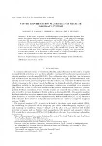
u (t ) f (•)

G (q)

y0 ( t ) +

+

y (t) = bT φ (t) a + v (t) ,

(5)

where a := b

:=

£

a1



φ1 (u (t − 1)) φ1 (u (t − 2)) .. .

£

  φ (t) :=  

a2

b1

b2

···

am

···

bn

¤T

¤T

,

,

··· ··· .. .

φm (u (t − 1)) φm (u (t − 2)) .. .

φ1 (u (t − n)) · · ·

φm (u (t − n))



  . 

Let us introduce a notation useful for a different formulation of the bilinearly £ parameterized linear ¤regression. For any matrix M = M1 M2 · · · Mm , the overlined notation M denotes the column vector obtained by stacking the columns M1 , M2 , ..., Mm , namely,   M1  M2    M =  . .  ..  Mm

y (t )

Fig. 1. A discrete-time Hammerstein model

This section shows that when appropriately parameterized, Hammerstein system identification can be formulated in the form of (1), which is a linear regression with bilinear parameters. In order to focus on the main issues of this paper, let us consider a single-input and single-output discrete-time Hammerstein system with a finite impulse response (FIR) linear part, as illustrated in Fig. 1 where u(t) and y(t) are respectively the input and the noise-corrupted output of the Hammerstein system. The case of infinite impulse response linear part can be addressed similarly using the separable LS technique; the details are omitted due to space limitation. More precisely, the FIR linear part G(q) in Fig. 1 is parameterized by b1 , . . . , bn such that n X bi x(t − i) + v(t). (2) y(t) = i=1

The additive noise v(t) is assumed to be white. The static nonlinearity f (·) is assumed to be a linear combination of known basis functions φi (·), m X aj φj (u(t)) . (3) x(t) = j=1

Here the orders n and m are assumed to be known a prior. Substituting the immeasurable inner signal x(t) in (3) into (2) yields a linear regression model parameterized in a bilinear form, m n X X bi aj φj (u(t − i)) + v (t) . (4) y(t) = i=1 j=1

In order to more clearly show that (4) is in the bilinear form (1), rewrite it as

With this notation, (5) can also be written as  T  b1 a1 φ1 (u (t − 1))  φ1 (u (t − 2))   b2 a1       .. ..    . .     φ1 (u (t − n))   bn a1       .. .. y(t) =    . .     φm (u (t − 1))   b1 am     φm (u (t − 2))   b2 am       .. ..    . . bn am φm (u (t − n)) T



         + v (t)       

= φ (t) baT + v (t) .

(6)

N {u (t) , y (t)}t=1 , define T  

For an input-output data set    φ (1) y (1) T   y (2)   φ (2)    Y = ,Φ =  .. ..   .  . T y (N ) φ (N )

v (1)   v (2)  ,V =   ..   .  v (N )



  , 

then (6) leads to Y = ΦbaT + V.

(7)

It is clear that these new notations are such that Y ∈ RN , Φ ∈ RN ×l and V ∈ RN with l = mn. Now let us introduce a standard assumption to remove the scale ambiguity between a and b and to make the parametrization unique. Assumption 1. The first non-zero entry of b is positive, and 2

kbk2 = bT b = 1.

(8)

With the above formulation, the identification of the Hammerstein system amounts to the estimation of the bilinear N parameters a and b from the data set {u (t) , y (t)}t=1 .

3621

ThA14.2 III. T HE TSA AND ITS OPTIMALITY RESULT

the solution of the unconstrained weighted linear LS problem (10a), namely, ¡ ¢ ˆ ) = ΦT W Φ −1 ΦT W Y. (11) θ(W

In this section we analyze the optimality property of the Two Stage Algorithm (TSA) after a recall of the algorithm. A. Weighted least squares criteria and the TSA For the estimation of the bilinear parameters a and b in (7), a traditional approach is to consider the weighted nonlinear LS criterion ´T ´ ³ 1³ min L(b, a, W ) = min ΦbaT − Y W ΦbaT − Y , b,a b,a 2 (9) where W ∈ RN ×N is some user-selected symmetric weighting matrix. To ensure the uniqueness of its solution, this LS problem should be solved under the constraints stated in Assumption 1. Since the TSA described later in this section provides a solution naturally satisfying these constraints, we will not always explicitly mention these constraints when the nonlinear LS problem (9) is referred to. The following assumption is also for ensuring the uniqueness of this nonlinear LS solution. Assumption 2. The matrices Φ ∈ RN ×l and W ∈ RN ×N are such that ΦT W Φ has full rank. Remark that this assumption implies that Φ has full column rank, a condition related to the excitation property of the system input. A positive definite weighting matrix W then ensures Assumption 2. Some positive semidefinite matrices W can also satisfy this requirement. Let us slightly reformulate the nonlinear LS problem (9) in order to make the connection with the TSA. By introducing the notation Θ := baT , the LS problem (9) is equivalent to the following one with a rank constraint, ¢T ¡ ¢ 1¡ (10a) ΦΘ − Y W ΦΘ − Y min L(Θ, W ) = min Θ Θ 2 s.t. rank (Θ) = 1. (10b) Some constraints equivalent to those of Assumption 1 should also be added for a unique solution of this LS problem. Remark that now in (10) the single parameter vector θ := Θ shows up quadratically in the weighted LS problem; however, the associated matrix Θ ∈ Rn×m has a rank constraint1 which is usually difficult to be taken into account in optimization problems. In this paper we are interested in a solution known as the TSA based on a relaxation approach. It first solves the unconstrained LS problem (10a) by omitting the rank constraint (10b) and then subsequently projects the solution onto the class of bilinear equations via the singularvalue decomposition (SVD). The following description of the TSA closely follows that in [2]. The Two Stage Algorithm (TSA) 1) Choose a weighting matrix W ∈ RN ×N and use it to estimate the parameter vector θ = Θ through 1 The

[9].

rank constraint was also referred to as the collinearity constraint in

ˆ 2) Build the matrix Θ(W ) ∈ Rn×m from the vector l ˆ θ(W ) ∈ R such that ˆ ). ˆ Θ(W ) = θ(W

Let σ1 be the largest singular value of the matrix ˆ Θ(W ), and u1 and v1 be its left and right singular vectors associated with σ1 , then the bilinear parameters a and b are estimated by ˆ a ˆ(W ) ˆ ˆb(W )

= s1 v1 ,

(12)

= s1 σ1 u1 ,

(13)

where s1 = ±1 is the sign of the first non-zero entry of u1 . Notes on Notations. •

•

•

The solution of the nonlinear LS problem (9) under Assumptions 1 and 2 will be noted as a ˆ(W ) and ˆb(W ). The solution Θ of the unconstrained weighted linear LS ˆ ). problem (10a), vectorized as θ = Θ, is noted as θ(W ˆ ˆ The results of the TSA are noted as a ˆ(W ) and ˆb(W ).

B. Optimality with special weighting matrices By omitting the rank constraint (10b), the solution set in (11) becomes broader than that of the optimization problem (10). For instance, as noticed by Goethals et al. [9], if ′ θi,j := bi aj is the solution of (10a), so is θi,j := bi aj + β α for any set of variables α , j = 1, · · · , m such that i j j Pm ∈ R, and any set of j=1 αj φj (u(t)) = constant, ∀t P n variables βi , i = 1, · · · , n such that i=1 βi = 0. However, the matrix   θ1,1 θ1,2 · · · θ1,m  θ2,1 θ2,2 · · · θ2,m     .. .. ..  ..  . . . .  θn,1 θn,2 · · · θn,m with θi,j := bi aj satisfies the rank constraint (10b), while the ′ corresponding matrix consisting of θi,j does not. Though in principle the TSA can provide the estimates of a and b for any weighting matrix W , it is not obvious if these estimates are the solution of the original LS problem (9) or if they minimize another error criterion. Hence, the significance of the solution given by the TSA is the main question this paper attempts to answer. This question has already been partly answered by Theorem 2.2 of [2] which is restated as follows. Theorem 1. If the weighting matrix W , used both in the nonlinear LS problem (9) and in the TSA, satisfies ΦT W Φ = αIl ,

(14)

where α is any positive scalar and Il is the l × l identity matrix, then the TSA produces the optimal solution of the

3622

ThA14.2 nonlinear LS problem (9), or more precisely (using notations introduced at the end of Section III-A), ˆˆ(W ), a ˆ(W ) = a ˆb(W ) = ˆˆb(W ). ¤ In [2] Theorem 1 was first presumed before being proved, and the proof therein does not indicate how this result has been derived. In contrast, the new proof here directly derives this result through the Lagrange multiplier approach, it is thus more constructive in this sense. Hopefully, this more constructive approach may allow some generalizations of the result in future works. Proof of Theorem 1. Consider the optimization problem (10a), replace the constraint (10b) by Θ = baT , and remind also the constraints (8). Then the optimization problem (10) is reformulated as ¢T ¡ ¢ 1¡ ΦΘ − Y W ΦΘ − Y min Θ 2 s.t. Θ = baT , and bT b = 1. Here Θ, a and b are all variables, and the criterion and constraints are both quadratic. The Lagrangian is ³ ´ ¢T ¡ ¢ 1¡ T L = ΦΘ − Y W ΦΘ − Y − Λ Θ − baT 2 ¢ 1 ¡ + µ bT b − 1 , 2 where Λ ∈ Rm×n and µ ∈ R are Lagrange multipliers. The first order optimality conditions are ¶T µ ¢ ¡ ∂L (15) = ΦT W ΦΘ − Y − Λ = 0, ∂Θ µ ¶T ∂L = Λa+µb = 0, (16) ∂b µ ¶T ∂L = ΛT b = 0. (17) ∂a For W satisfying (14), (15) becomes αΘ = ΦT W Y + Λ. By introducing a matrix Z ∈ Rm×n to associate with Z := ΦT W Y , we obtain αΘ = Z + Λ. Replacing Θ by baT yields αbaT = Z + Λ. T

(18) T

Using (17), (18) lead to αab b = Z b, which, by the assumption bT b =1 in (8), reduces to αa = Z T b.

(19)

Substitute (19) into (16) and into (18) (to remove a) and obtain respectively T

ΛZ b + αµb = 0,

(20)

bbT Z = Z + Λ.

(21)

or equivalently ¡ ¢ ZZ T b = bT ZZ T b + αµ b,

(22)

by noticing that bT ZZ T b is a scalar. If b 6= 0, it must be an eigenvector of ZZ T . On the other hand, let b be an eigenvector of ZZ T associated with the eigenvalue λ, that is ZZ T b = λb. Then (22) becomes ¡ ¢ λb = bT ZZ T b + αµ b ¡ ¢ = bT λb + αµ b = λb + αµb,

which, together with the facts that bT b =1 and α > 0, implies µ = 0. By Lemma 1 presented below, the error criterion in (9) is minimal if λ is the largest eigenvalue of ZZ T . To summarize, the first order conditions (15)-(17) are satisfied by ˆb that is the normalized eigenvector of ZZ T associated with the largest eigenvalue, i.e., ZZ T ˆb = λmaxˆb, as well as, a ˆ=

1 Tˆ Z b, α

(23)

(24)

T Θ= ˆbˆ aT and the Lagrange multipliers Λ = ˆbˆb Z − Z and µ = 0. Notice that Z = ΦT W Y is in fact the unconstrained weighted LS solution of Θ. By the well-known connection between the eigen-decomposition and the SVD, therefore, ˆb in (23) and a ˆ in (24) respectively are exactly the same as those in (12) and (13) from the TSA. ¤ Lemma 1. The error criterion in (9) is minimal if ˆb is the eigenvector of ZZ T associated with its largest eigenvalue λmax . Proof of Lemma 1. Let b be the eigenvector of ZZ T associated with the eigenvalue λ, i.e., ZZ T b = λb, and a = α1 Z T b. For simplicity of notation, introduce a new definition

1 T bb Z. α The error criterion in (9) becomes ´T ´ ³ 1³ L (b, a, W ) = W ΦbaT − Y ΦbaT − Y 2 1 T T = (η Φ W Φη − η T ΦT W Y 2 −Y T W Φη + Y T W Y ) ¢ 1 1¡ T = αη η − 2η T Z + Y T W Y , (25) 2 2 η := baT =

where the last equality uses (14) and the definition of Z, namely, Z = ΦT W Y . It is straightforward but tedious to show that

and ηT Z

=

Right-multiplying each term of (21) by Z T b and combining the result with (20) give

=

bbT ZZ T b = ZZ T b − αµb,

=

3623

1 T T bb Z Z α ¢T 1¡ ZZ T b b α 1 λ, α

ThA14.2 to restrain P and Q so that (27) is satisfied. Develop ΦT W Φ while reminding UΦT UΦ⊥ = 0 :

and 1 T T T bb Z bb Z α2 ´T 1 ³ T T = bb ZZ b b α2 1 = λ. α2 Therefore, the error criterion in (25) becomes ηT η

=

ΦT W Φ

λ 1 + Y TWY . 2α 2 Remind that this equality has been achieved for any eigenvalue of ZZ T , thus L (b, a, W ) achieves the minimal for λ = λmax . ¤

This result shows that ΦT W Φ is independent of Q. From (27), it follows that VΦ SΦ P P T SΦ VΦT SΦ P P T SΦ PPT

C. Parametrization of the special weighting matrices In [2], nothing was said about the construction of the special weighting matrices satisfying condition (14). In order to fill this gap, a complete parametrization of W satisfying (14) is given in Proposition 1 next. Proposition 1. For any full column rank Φ ∈ RN ×l with N ≥ l and any W ∈ RN ×N satisfying (14), there exist at least one VP ∈ RN ×l satisfying VPT VP = Il and one Q ∈ R(N −l)×N so that W is parameterized by Q and VP as ³ ´³ ´T −1 T −1 T W = α UΦ SΦ VP +U ⊥ UΦ SΦ VP +U ⊥ , (26) ΦQ ΦQ where UΦ , SΦ and UΦ⊥ are from the full SVD of Φ, ¤£ ¤T T £ SΦ 0 VΦ . Φ = UΦ UΦ⊥

(27)

for any given Φ ∈ RN ×l . Note that l denotes the number of columns £of Φ, and l ¤= mn for the Hammerstein model in (4). Let UΦ UΦ⊥ be the matrix containing the full left singular vectors of Φ, with UΦ ∈ RN ×l corresponding to the economic-size part, i.e., the full SVD of Φ is ¤£ ¤T T £ SΦ 0 VΦ . (28) Φ = UΦ UΦ⊥ For any positive semidefinite matrix W ∈ RN ×N , there exists at least one matrix R ∈ RN ×N such that

(29)

Any R ∈ RN ×N can be decomposed as R = UΦ P + U ⊥ Φ Q, l×N

(30) (N −l)×N

= Il , = Il , −2 = SΦ .

(31)

The last equation implies that the singular values of P are the −1 diagonal elements of SΦ and that the left eigenvectors of P form the identity matrix, or more clearly, the economic-size SVD of P is T P = Il S −1 (32) Φ VP . Therefore, the free parameter of P is the unitary matrix VP ∈ RN ×l . Conversely, it is easy to check that, for any VP ∈ RN ×l satisfying VPT VP = Il and any Q ∈ R(N −l)×N , the weighting matrix built through (32), (30) and (29) satisfies (27). This completes the proof. ¤ IV. E XAMPLE

Conversely, for any VP ∈ RN ×l satisfying VPT VP = Il and any Q ∈ R(N −l)×N , the weighting matrix W given by (26) satisfies (14). Proof of Proposition 1. To simplify discussions, the scalar parameter α can be dropped, since it is just a matter of scaling W by α. Then the goal of this appendix is to find a parametrization of W covering all the cases such that

W = RRT .

³ ´ VΦ SΦ UΦT UΦ P + U ⊥ ΦQ ³ ´T · UΦ P + U ⊥ UΦ SΦ VΦT ΦQ

= VΦ SΦ P P T SΦ VΦT .

L (b, a, W ) = −

ΦT W Φ = Il ,

=

with two matrices P ∈ R and Q ∈ R . Thus any W can be parameterized by P and Q, even though this parametrization may not be unique. Now the question is how

This section presents a numerical example to verify the theoretical results in Section III. Example 1. For the Hammerstein model in Fig. 1, y (t) x (t)

= G (q) x (t) + v (t) ¡ ¢ = 0.4472q −1 − 0.8944q −2 x (t) + v (t) ,

= u (t) + 2u2 (t) + 5u3 (t) + 7u4 (t) + u5 (t) .

The noise v (t) is a zero-mean white Gaussian noise with £ ¤T 0.4472 −0.8944 satisfies variance σv2 . Here b = Assumption 1 so that the parametrization of a and b is unique. The input u (t) is generated by passing a fixed realization of uniformly-distributed processes with magnitude range [−3, 3] through the filter 1/(1 − 0.5q −1 ), so that u (t) covers sufficient nonlinear ranges of the input nonlinearity. 100 Monte Carlo simulations are implemented, where each simulation takes a different realization of v (t). Two groups of estimates of a and b are obtained by the TSA and by directly solving the nonlinear weighted LS problem (9) using the “lsqnonlin” function of the Matlab Optimization Toolbox. The nonlinear LS problem is sensitive to initial estimates; hence the true parameters a and b are used to initiate “lsqnonlin” for the purpose of comparison. Table I list the mean and the standard deviations of the estimates in 100 Monte Carlo simulations, for the noise level σv2 = 1. The means of the associated loss functions L (b, a, W ) defined in (9) are listed as well at the bottom row in Table I. In each simulation, 100 data points of u (t) and y (t) are collected, i.e., N = 100.

3624

ThA14.2 TABLE I E STIMATES OF a AND b AND ASSOCIATED LOSS FUNCTIONS 2 = 1 σv · ¸ 0.4472 b =  −0.8944  1.0000    2.0000   a =   5.0000   7.0000  1.0000 L (b, a, W )

TSA ·

0.4473 ± 0.0013  −0.8944 ± 0.0006  0.9895 ± 0.1599  1.9932 ± 0.0777     5.0016 ± 0.0477     7.0004 ± 0.0058  0.9998 ± 0.0027 0.0302

¸

R EFERENCES

lsqnonlin · ¸ 0.4473 ± 0.0015  −0.8944 ± 0.0019  0.9897 ± 0.1616    1.9931 ± 0.0781   5.0014 ± 0.0383     7.0002 ± 0.0128  0.9997 ± 0.0045 0.0302

The estimates in Table I appear unbiased and consistent, as proved by Theorem 2.1 in [2]. Since “lsqnonlin” takes the luxury of using the true parameters a and b as the initial estimates, the global optima are expected. The resulting estimates are close to the counterparts from the TSA; in fact, the two loss functions L (b, a, W ) are exactly the same, which validates the conclusion in Theorem 1. In Table I, the weighting matrix W in (26) is used with the arbitrary matrix Q in (30) set to zero, and the unitary matrix Vp in (32) randomly-generated. When Q is the zero matrix, the unitary matrix Vp has no effects on the estimates; this can be seen by representing θˆ (W ) in (11) in terms of the SVD of Φ in (28) and the complete parametrization of W in (29):

= = = =

θˆ (W ) ¡ T ¢−1 T Φ WΦ Φ WY ¢ ¡ ¢¡ ¢T ¡ T T UΦ P + UΦ⊥ Q UΦ P + UΦ⊥ Q Y UΦ SΦ VΦ ¡ ¢T ´ ¢³ ¡ Y VΦ SΦ UΦT UΦ P P T UΦT + UΦ P QT UΦ⊥ ³ ´ ¢ ¡ T −1 T V Φ SΦ UΦ + Vp QT UΦ⊥ Y.

Here the second and third equalities use (14) and UΦT UΦ⊥ = 0, respectively, and the last one is from (31) and (32). If a non-zero matrix Q is used, the two loss functions L (b, a, W ) are still the same, which is consistent with Proposition 1. Simulation results reveal that the selection of Vp and Q do matter to the accuracy of estimated results; however, the general selection guideline is now unclear to us. V. C ONCLUSION This paper revisited the TSA for identification of Hammerstein systems. A known result is recalled in Theorem 1: for some special weighting matrices satisfying the equality (14), the TSA provides the solution of a weighted nonlinear LS problem (9), or equivalently, of a weighted linear LS problem (10a) subject to a rank constraint (10b). This result was re-derived in this paper in a constructive manner based on Lagrange multipliers, whereas originally in [2] it was first assumed before being proved. Our constructive proof may hopefully allow to generalize the obtained result to other weighting matrices, even though it is not successful for the time being. We also give a complete parametrization of the special weighting matrices. The theoretical results were validated via a simulation example of identification of Hammerstein systems.

[1] R. Abrahamsson, S.M. Kay, & P. Stoica (2007). Estimation of the parameters of a bilinear model with applications to submarine detection and system identification. Digital Signal Processing, vol.17, pp.756773. [2] E.W. Bai (1998). An optimal two-stage identification algorithm for Hammerstein-Wiener nonlinear systems. Automatica, vol.34, no.3, pp.333-338. [3] E.W. Bai, & Y. Liu (2006). Least squares solutions of bilinear equations. Systems & Control Letters, vol.55, pp.466-472. [4] A. Balestrino, A. Landi, M. Ould-Zmirli, & L. Sani (2001). Automatic nonlinear auto-tuning method for Hammerstein modeling of electrical drives. IEEE Trans. Industrial Electronics, vol.48, no.3, pp.645-655. [5] F. Chang, & R. Luus (1971). A noniterative method for identification using Hammerstein model. IEEE Trans. Automat. Contr., vol.16, no.5, pp.464-468. [6] S. Cohen, & C. Tomasi (1997). Systems of bilinear equations. Technical report, Computer Science Dept., Stanford Univ., Standard, CA. [7] E.J. Dempsey, & D.T. Westwick (2004). Identification of Hammerstein models with cubic spline nonlinearities. IEEE Trans. Biomed. Eng., vol.51, no.2, pp.237-245. [8] E. Eskinat, S.H. Johnson, & W.L. Luyben (1991). Use of Hammerstein models in identification of nonlinear systems. A.I.Ch.E. J., vol.37, no.2, pp.255-268. [9] I. Goethals, K. Pelckmans, J.A.K. Suykens, & B. De Moor (2005). Identification of MIMO Hammerstein models using least squares support vector machine. Automatica, vol.41, pp.1263-1272. [10] J.C. Gomez, & E. Baeyens (2004). Identification of block-oriented nonlinear systems using orthonormal bases. J. Process Control, vol.14, no.6, pp.685-697. [11] J.C. Gomez, & E. Baeyens (2005). Subspace-based identification algorithms for Hammerstein and Wiener models. Eur. J. Control, vol.11, pp.127-136. [12] R. Haber, & L. Keviczky (1999). Nonlinear System Identification: Input-Output Modeling Approach, Dordrecht: Kluwer Academic Publishers. [13] A. Janczak (2005). Identification of Nonlinear Systems Using Neural Networks and Polynomial Models: A Block-Oriented Approach, New York: Springer-Verlag. [14] F. Jurado (2006). A method for the identification of solid oxide fuel cells using a Hammerstein model. J. Power Sources, vol.154, no.1, pp.145-152. [15] T. McKelvey, & C. Hanner (2003). On identification of Hammerstein systems using excitation with a finite number of levels. Proc. of the 13th International Symp. on System Identification (SYSID2003), pp.5760. [16] G. Mzyk (2000). Application of instrumental variable method to the identification of Hammerstein-Wiener systems. 6th International Conf. MMAR, Miedzyzdroje. [17] H.J. Palanthandalam-Madapusi, D.S. Bernstein, & A.J. Ridley (2006). Subspace identification of periodically switching Hammerstein-Wiener models for magnetospheric dynamics. 14th IFAC Symp. on System Identification, Newcastle, Australia, pp.535-540. [18] H.J. Palanthandalam-Madapusi, A.J. Ridley, & D.S. Bernstein (2005). Identification and prediction of ionospheric dynamics using a Hammerstein-Wiener model with radial basis functions. 2005 American Control Conf., Portland, OR, USA, pp.5052-5057. [19] R. Srinivasan, R. Rengaswamy, S. Narasimhan, & R. Miller (2005). Control loop performance assessment. 2. Hammerstein model approach for stiction diagnosis. Ind. Eng. Chem. Res., vol.44, no.17, pp.6719-6728. [20] S.W. Sung (2002). System identification method for Hammerstein processes. Ind. Eng. Chem. Res., vol.41, no.17, pp.4295-4302. [21] J. Wang, A. Sano, T. Chen, & B. Huang (2009). Identification of Hammerstein systems without explicit parameterization of nonlinearity. Int. J. Control, vol.82, no.5, pp.937-952, 2009. [22] J. Wang, Q. Zhang, & L. Ljung (2009). Optimality analysis of the two-stage algorithm for Hammerstein system identification. 15th IFAC Symposium on System Identification (SYSID2009), pp.320-325.

3625