Dec 1, 2009 - may only be feasible for a subset of the traffic in the ether. ..... GNU Radio [14] is an open source software toolkit for building software radios.
RFDump: An Architecture for Monitoring the Wireless Ether Kaushik Lakshminarayanan, Samir Sapra, Srinivasan Seshan, Peter Steenkiste Carnegie Mellon University Pittsburgh, PA 15213
{kaushik, ssapra, srini, prs}@cs.cmu.edu Abstract
1. INTRODUCTION
Networking researchers have been using tools like wireshark and tcpdump to sniff packets on physical links that use different types of datalink protocols, e.g. Ethernet or 802.11, allowing them to monitor higher level protocols sharing these links. However, monitoring wireless links is more challenging, since the transmission medium is shared by flows using diverse datalink protocols (e.g. 802.11, Bluetooth) and physical layer schemes (e.g. QPSK and GFSK). To this end, we propose RFDump, a software architecture for monitoring packets on heterogeneous wireless networks. The key idea underlying our architecture is the use of a fast detection stage which can tentatively map signals to protocols very efficiently. As a result, RFDump can scale up to a modest number (5-10) of wireless technologies. We implemented RFDump on the GNU Radio and USRP platforms. This is, to our knowledge, the first inexpensive software-based infrastructure for simultaneously analyzing multiple wireless protocols in real-time. Using traces from the real world and from a wireless emulator testbed, we show that our implementation is efficient and accurate. Further, we demonstrate that our system is extensible and scales with the addition of new protocols.
Tcpdump, Wireshark/Ethereal and similar applications have become a critical part of the tool collections used by networking researchers, networking administrators and application developers. These tools expose the operation of a network in a detailed, cross-layer fashion. Based on this exposed information, users are able to monitor and analyze the interactions between different nodes, different protocols, different protocol layers and different applications in the network. This has enabled activities such as diagnosing network protocols, optimizing network performance and even teaching network protocol operation. Unfortunately, applying these tools in wireless networks fails to provide the same level of insight into the operation of the network. There are two reasons for this problem. First, these tools operate at the link-layer and above. In wireless settings, the behavior of the physical layer is critical to the operation of the network. Second, these tools are limited to operation over a single network interface card (NIC), such as an 802.11 NIC. As a result, they can only report on the detailed operation of the associated network link technology. However, unlike wired networks, the physical medium over which the network operates is shared by many link technologies. For example, the 2.4 GHz unlicensed spectrum band is shared by 802.11, Bluetooth, ZigBee, cordless phones and a wide range of other link technologies. Making observations on a single link technology hides many of the node, protocol and application interactions that users are attempting to observe with such tools. In this paper, we describe the design of RFDump, a tool that extends the monitoring capabilities below the link layer and enables more effective monitoring of the wireless ether. In order to be practical, a monitoring tool for wireless networks must meet two key requirements. First, we must be able to monitor packets that use a wide variety of protocols, so the tool must efficiently support multiple protocols and it must be easy to add new protocols in the future. Second, the tool must run in real-time so it can be used for runtime analysis and troubleshooting. Note that we do not expect our system to interact with the monitored links (i.e., it does not need to implement the link-layer protocol). As a result, our system can process transmissions after some delay (e.g., a second) but the processing must keep up with the rate of packet transmissions. In addition, while core functions, such as identifying packets and the technology they use, must occur in real time, more complex functions, such as full decoding of payloads or deep packet inspection, may only be feasible for a subset of the traffic in the ether.
Categories and Subject Descriptors C.4 [Performance of Systems]: [Measurement Techniques]; C.2.1 [Computer-Communication Networks]: Network Architecture and Design—Wireless Communication; C.2.3 [Computer-Communication Networks]: Network Operations—Network monitoring
General Terms Measurement, Experimentation, Performance
Keywords software defined radio, wireless networks, monitoring, WiFi, Bluetooth, tcpdump
Permission to make digital or hard copies of all or part of this work for personal or classroom use is granted without fee provided that copies are not made or distributed for profit or commercial advantage and that copies bear this notice and the full citation on the first page. To copy otherwise, to republish, to post on servers or to redistribute to lists, requires prior specific permission and/or a fee. CoNEXT’09, December 1–4, 2009, Rome, Italy. Copyright 2009 ACM 978-1-60558-636-6/09/12 ...$10.00.
GNU Radio Block 802.11 demodulation (1 Mbps) Bluetooth demodulation Peak/Energy detection
CPU time / Real time 0.6 0.7 0.05
Table 1: Time taken by some blocks
Figure 1: The na¨ıve architecture
This may not seem like a significant challenge since tools such as Tcpdump are able to decode a wide range of protocols efficiently. The key to this efficiency is that each protocol layer specifies the protocol used by its contents. For example, the IP header contains a protocol field that identifies the transport protocol of the datagram contents. This allows Tcpdump to run just the code needed to decode the appropriate protocol. Unfortunately, the physical layer does not explicitly identify the protocol used by an active transmissions. Instead wireless networking cards use a combination of preambles, modulation and coding schemes, and header information to determine the protocol. As a result, the most obvious and na¨ıve solution (Figure 1) to performing wireless monitoring would require that we monitor all link-layers in parallel (i.e. try to interpret every signal with every protocol). This solution is either expensive (for hardware) or slow (for software). The core of our design is the decomposition of the problem into a detection stage followed by the demodulation stage. The detection stage can tentatively map signals to protocols very efficiently – essentially providing a protocol tag much like the ones that Tcpdump relies upon. We rely on some key observations to make these detection modules much more light-weight than complete demodulation. First, these detectors can operate with some delay, which enables the use of algorithms that are not appropriate for demodulation. Second, unlike demodulators, these detectors are allowed to have false positives. If that happens, the signal is passed to demodulation code to interpret the content of the transmission and the demodulator will then determine that the signal does not represent a valid packet for that protocol. This paper makes three contributions. First, we present the RFDump architecture for monitoring diverse wireless links. The architecture introduces a light-weight detection stage before demodulation so that demodulation needs to be performed only on actual RF transmissions. Second, we introduce a specific set of fast early detectors for devices using 802.11b/g and Bluetooth, as well as other RF devices such as microwave ovens. Finally, we present a prototype implementation of the RFDump architecture on the GNU Radio [14] and USRP [17] software defined radio (SDR) platforms. Our implementation is an early prototype (limited in various ways by the underlying hardware platform we use) used to evaluate the potential benefits of the architecture. We compare its performance with a na¨ıve solution and show that our architecture is much more efficient, while maintaining the same level of accuracy. We not only detect most of the packets detected by the na¨ıve solution, but also packets
which cannot be demodulated due to the limitations of the USRP interface. Although the individual detection modules themselves play a key role in achieving efficiency and scalability, the main contribution of the paper lies in how the architecture is designed for monitoring different types of wireless link technologies in an efficient manner. The rest of the paper is structured as follows. The next section presents the RFDump architecture and Section 3 describes our early detection modules that can detect packets belonging to a number of protocols without demodulating and decoding. Section 4 describes the implementation of the architecture on the GNU Radio and USRP framework. Section 5 evaluates our implementation for efficiency and accuracy by comparing it with straightforward but na¨ıve alternatives. Section 6 compares our architecture with alternate approaches and we summarize our work in Section 7.
2. ARCHITECTURE 2.1 Motivation and Requirements Monitoring wireless networks is difficult because activity on the transmission medium (the ether) is difficult to observe and decode. The problem is that unlicensed spectrum is open to anybody with only minimal limitations, and as a result, a wide variety of physical and datalink layers are in use. Nevertheless, it is important to get a full picture of the activity in the shared spectrum. For example, when diagnosing Wi-Fi problems, a full picture is critical because non-Wi-Fi users can reduce the (Wi-Fi) network capacity by reducing transmission opportunities or, even worse, cause high packet error rates if the technologies cannot coexist. This leads to the following requirements for a wireless monitoring tool. • Multi-protocol: it must support simultaneous monitoring of at least a small (e.g. 5-10) number of protocols and RF sources. • Real-time: it must perform core functions, e.g. identifying packets and the technology they use, in real time. • Protocol Extensible: it must be relatively simple to add support for new protocols, e.g. 802.11n. • Functionality Extensible: it should be possible to add additional modules that further analyze traffic, e.g. demodulator, diagnostic modules, deep packet inspection. Unless otherwise specified, we refer to the process of demodulation, decoding and analysis together as demodulation for the rest of the paper. Given these high-level requirements, let us consider the suitability of the na¨ıve architecture shown in Figure 1. Here, the entire input stream is sent to demodulators for all technologies that may be in use. Implementing this architecture using separate hardware for each demodulator is both
Figure 2: Illustration of RFDump architecture expensive and impractical (e.g. conflicting drivers, accommodating many cards on a single machine). An alternative is to use a software defined radio (SDR) and perform demodulation in software. Unfortunately, demodulation in software is a computationally expensive operation and the system in Figure 1 would not scale to even a modest number of protocols. The first two rows of Table 1 show how slow demodulation is compared to real time; these numbers are for GNU Radio processing a sample stream generated by a USRP radio at 8 million samples per second on a 2.13 GHz Core 2 Duo processor (see Section 4.1 for details). Even with a faster platform, this approach will not scale to 5-10 protocols, especially if we also want to support higher speed protocols such as 802.11g and 802.11n. With advancements in software radios, we expect the size of the input data stream per unit time (∼480 Mbps for USRP to ∼1 Gbps for USRP2) to go up over time. To be able to sustain real-time throughput, we need to make the analysis phase very efficient. For example, we need to limit the number of accesses to the data stream to reduce load on the memory system, avoid redundant computation, and discard uninteresting blocks of samples as early as possible in the process. An obvious optimization to the above design is to reduce the load on the demodulators by using an energy-based filtering stage before demodulation. This filter would only pass blocks of samples that exceed a minimum energy threshold so the demodulators would only be applied to the parts of the sample stream that are likely to include useful signals. The “energy detection” row in Table 1 shows that energy detection is a cheap operation compared to demodulation. After the energy detection stage, the demodulation cost will scale with the level of activity in the ether, i.e. if the ether is busy 20% of the time, the demodulation cost would be reduced by a factor of five compared with the na¨ıve architecture. While a big step forward, this solution still does not scale to even a modest number of protocols. Even worse, its
cost will be high (comparable to that of the na¨ıve architecture) when the ether is very busy, which is likely when monitoring is most critical.
2.2 Architecture Overview RFDump extends upon the energy filtering-based na¨ıve design by improving the filtering of the signal. Instead of simply passing all signals, or all signals above some energy threshold, to all demodulators, the RFDump architecture attempts to only pass signals that are of a particular technology on to the appropriate demodulators/analyzers. This ensures that minimal amount of work is done in demodulating signals. While the task of classifying signals is obviously a subset of demodulating a signal, this design does raise the concern of how to efficiently classify signals to a particular technology. As we show in this paper, the process of classifying signals (i.e. detecting activity of a specify technology) is much more light-weight than full demodulation. We believe that this will always be true for a few reasons beyond just the relative complexity of the tasks. First, the architecture tolerates false positive classification errors gracefully. The goal of the classification stage is to reduce the amount of work done by the demodulators. As a result, as long as it is filtering signals relatively effectively, passing a few extra signals will not impact the correct operation of the design. Second, unlike typical demodulation applications, our target application accommodates some latency (but not throughput degradation) in processing the signal. We believe that classification can make far greater use of this delay tolerance than demodulation or other analysis tasks. As we show in the remainder of this paper, this enables the creation of very light-weight classification schemes. Figure 2 illustrates the RFDump architecture that implements the above design. Our architecture broadly consists of a detection stage and an analysis stage. We further divide the detection stage into a protocol-agnostic detection
stage and a protocol-specific detection stage. The protocolagnostic detection stage identifies properties of blocks of samples that could be of interest to multiple protocols and associates confidence values with these properties. This is a concise representation of the sample stream and it is stored separately as metadata associated with each block of samples. A simple example of a protocol-agnostic detection stage is a peak detector that reports the start and end times of RF transmission. The protocol-specific modules in the next stage use the information from the protocol-agnostic stage to determine which blocks of samples could be part of a packet of a particular protocol, and they selectively forward only those blocks of samples to the analysis phase for the respective protocols. The protocol-specific modules in the detection stage typically access the metadata from the previous stage and the same metadata will often be reused by multiple protocol-specific modules. An example of protocolspecific processing might be to examine the peaks reported by the peak detector to identify timing behavior specific to a protocol. After the detection stage, the stream of signal is only accessed as needed, i.e. uninteresting blocks of samples are discarded, while promising blocks are only read if further analysis (e.g. demodulation) is needed. In our implementation, the analysis stage typically demodulates Wi-Fi and Bluetooth signals, but other analysis tools could be used, e.g. demodulation of headers only. RFDump meets the requirements listed in Section 2.1. For an architecture to support 5-10 protocols, the incremental cost (CPU cycles spent) for additional protocols should be low. The reason is that the functionality of the first phase of detection is protocol-agnostic (e.g. a peak detector) and is shared by multiple protocols. The protocol-specific detection stage is also inherently fast as it works at a much coarser granularity – it only operates on the meta data. Adding support for more protocols is usually easy since the code in the protocol-specific detectors typically performs just simple operations on the metadata created by already existing protocol-agnostic modules. For example, many different protocols can make use of the output of a peak detector to perform relatively simple time-based detection schemes. As we show later, the same is true for phase-based and frequency-based detection. One nice property of our system is that we can mostly use existing demodulation code (e.g. BlueSniff [15] and BBN’s 802.11 demodulator [1]). Developers would simply need to implement appropriate detection code, which tends to be far less complex than demodulation, to add such existing analysis/demodulation code to the system. Note that the RFDump architecture in Figure 2 (similar to the na¨ıve architecture) has inherent parallelism that can be exploited using multi-threading. This is, of course, important on today’s multi-core CPUs. Unfortunately, our platform (GNU Radio) currently does not support multithreading, so the measurements in this paper only use a single core.
3.
EARLY DETECTION MODULES
We now describe the early detection modules we used in our prototype system. They can tentatively map signal belonging to 802.11b, Bluetooth, and microwave ovens. We also discuss how the modules can be extended to support other protocols.
Protocol (Mbps) b (1) 802.11 b (2) b (5.5/11) g
a
Timing
Phase
(µs)
(Modulation)
Slot 20 20 20 9
SIFS 10 10 10 10
Channel width
Scheme Spreading (MHz) DBPSKa Barker DQPSKa Barker 22 DQPSKa CCK OFDMbc 20
Bluetooth
Slot 625
GFSK
802.15.4 (ZigBee)
Slot IFS 320 192/600
QPSK
Residential Microwave
AC cycle 16667/20000
FHSS
1 5 10-75
Preamble is sent using DBPSK
b CTS-to-self packets use one of the 802.11b rates c
Uses BPSK, QPSK, 16-QAM or 64-QAM for the subcarriers
Table 2: Relevant features for different wireless protocols in the 2.4 GHz ISM band
3.1 Fast Early Detection We require that fast detection modules for our architecture to be extensible to a range of, including future, wireless technologies. As described earlier, the goal of the fast detectors is to efficiently identify key properties of the signal that can be used to tentatively map sample blocks to possible protocols. An important challenge in the design of fast detectors is to determine the right tradeoff between (a) maximizing the level of accuracy and confidence in the information that is extracted and (2) minimizing the processing and memory access cost. For example, submitting the signal to a group of demodulators may yield detailed and accurate information, but it is very expensive. We need much cheaper detectors, even if this reduces the confidence in the results slightly. Our current prototype includes fast detectors for time, phase, and frequency analysis of the signal samples to detect packets of different wireless standards. Table 2 shows some relevant frequency, timing, and phase properties of wireless protocols in the 2.4 GHz ISM band that can be used for their detection. To see how these properties are used in the fast detection stage, consider the row corresponding to one of the protocols, say 802.11b (2 Mbps). We have a protocol-agnostic peak detection module that identifies the timing between RF transmissions. This timing information is passed on to all protocol-specific modules and any new protocol added will reuse the computation of the peak detection module for timing-based detection. The protocolspecific timing module for this variant of 802.11b could look for RF transmissions that were spaced by 10 µs which would suggest transmissions spaced by the 802.11 SIFS. Similarly, we can have a set of protocol-agnostic modules that look for the use of specific forms of phase modulation (e.g. DBPSK, DQPSK). The protocol-specific module could use this to identify signals that used a combination of DBPSK, which is used in 802.11b’s PLCP preamble, and DQPSK, which is used to transmit 802.11b data. Note that the results of the protocol-agnostic module could also used by a ZigBee protocol-specific detection block, which uses QPSK, and by other forms of 802.11, which use different combinations of DBPSK and DQPSK.
Figure 3: SIFS timing in 802.11 It is important to consider the computational complexity of the detection blocks. For example, if analyzing the phase of the signal at this level is too expensive, a lighter weight analysis that just detects a pattern in the phase may be sufficient to perform effective classification of the signal. Note that the frequency, phase, and timing detectors that we present in this paper are just simple examples of detection blocks that our system can use. It is likely that other, possibly more efficient detectors will be identified over time. The simplest design for RFDump would simply apply the fast detectors to the full signal stream. There are however two simple techniques that can be used to further reduce the overhead of the detection stage. The first technique is a simple energy detector that discards blocks of signals that are below a certain level (e.g. at the noise floor). This can significantly reduce processing costs, especially if there is a low level of spectrum utilization. This is especially useful when scanning, e.g. a single radio looks at multiple frequency bands over time, since efficiency is then a concern even for idle bands. Filtering based on energy detection should be conservative: it should not discard short burst of low-energy samples that sit between two sample blocks of interest. A second technique is to use sampling: when analyzing a burst of samples with consistent signal strength, it may be sufficient for the fast detectors to only look at a subset of the samples. This helps further reduce the cost of the detection stage, with minimal impact on accuracy and confidence. Our current prototype implements energy detection but does not use sampling. In the following sections, we describe the design of our timing, phase and spectrum fast detectors. Note that many of the algorithms used by these detectors are well known. The key novelty of the design is how the detectors leverage properties such as tolerance to delay and false positives (explained in Section 2.2) in the detection stage to provide a light-weight mechanism to classify the signals.
3.2 Timing Analysis Most wireless protocols define timing information like Interframe Space (IFS) and slot times. For example, in 802.11, a packet and the MAC-level acknowledgment have a time gap corresponding to SIFS (Short Interframe Space) as shown in Figure 3; whenever there is contention, 802.11 packets are separated by a time interval of DIFS + k×ST, where DIFS is the Distributed Interframe Space, k ∈ [0, CW], CW is the contention window and ST is the slot time; in Bluetooth, packets are sent in TDD (Time Division Duplex) slots of
625 µs (1600 hops in a second), with the master and slave alternating. Similar timing properties have been used for service discovery and device identification in the context of spectrum management in cognitive networks [11]. Much like RFDump, spectrum management applications do not need to meet protocol-level timing requirements. In fact, since these applications have weaker performance requirements, they use even coarser grain and slower timing-based pattern search (e.g., by using AP’s beacon spacing). Our work shows that timing-based pattern recognition can be extended even further and can meet the real-time requirements of RFDump. In the time domain, we need to find the spacing between peaks (packets) and correlate it to different protocols. We divide this process into two parts – a single protocol-agnostic peak detector block, and protocol-specific peak and gap analysis blocks, one for each protocol. The peak detection block computes the running average of energy over a window of consecutive samples. Based on empirical thresholds for energy level of the current window of samples, the previous window of samples, and the noise floor, the protocol-agnostic module determines the beginning and the end of peaks. Samples are averaged to reduce the chance that noise would cause the detector to split up a peak (packet) into multiple shorter ones. It communicates with the analysis modules by passing metadata containing succinct information regarding the peaks detected in every fixed chunk of samples along with a pointer to the history of peaks detected. The history is an array of starting and ending timestamps of recent peaks and it is useful for finding both the length of peaks and the time gap between consecutive peaks. By having a protocolagnostic peak detection block do all the computation on the input stream, we reduce the load on the protocol-specific detectors, which work only on the metadata. Extending timing analysis to future protocols requires the minimal work of writing a protocol-specific block for comparing the peaks and spacings with values that apply to the new protocol. For example, a ZigBee timing block would look for spacings that are a multiple of backoff periods (slot time), LIFS (Long Interframe Space), Short Interframe Space (Short Interframe Space) or tACK (Time between a packet and the MAC-level ACK). A microwave timing block might look for peaks occurring at the rate of AC frequency (60 Hz, i.e. once every 16.67 ms). Some protocol-specific blocks may require deeper analysis such as correlating signal strengths (which are present in the metadata). For example, since the emitted signal from a residential microwave has constant power, we can use signal strength information to verify whether the amplitude of the signal is constant across peaks.
3.3 Phase Analysis A number of protocols use some form of phase modulation. The idea of the phase analysis module is to determine the phase of the samples in the sample stream and to identify whether a particular pattern is present. Different levels of analysis may be used with different precision versus overhead tradeoffs. The simplest check could be to simply determine whether a pattern is present or not; the value of this information is limited to determine whether the protocol uses phases modulation or not. A more balanced alternative is to determine the specific modulation scheme. For example, QPSK and DPSK will result in specific phase
3.4 Frequency Analysis
Figure 4: Estimating constellation
values dominating. GMSK, which changes phase incrementally, will have discrete values for the first derivative of the phase. An even more aggressive analysis may determine the type of coding is used; this is however unlikely to appropriate for a fast detection stage. Two additional issues need to be considered during the phase analysis. First, different protocols can use different symbol rates, which must be considered by the analysis. Of course, the symbol rate is also an identifying feature of a protocol. Second, the center frequency of the signal under investigation may be offset relative to the center frequency of the frequency range being sampled. This results in a constant drift of the phase over time. Again, this is useful information since the drift allows us to determine what channel is used by the protocol packet. To illustrate how phase information can be computed cheaply, consider the following scenario: Assume our RF frontend outputs complex values representing the observed signal, sampled and translated down to some intermediate frequency (IF). Also assume the band being monitored contains a PSK signal, though possibly at a different center frequency (what follows can be generalized to QAM). Now, with one arctan operation per sample we get the phase of the IF signal. The frequency offset between monitored band and PSK signal will contribute a constant to the first derivative of this IF phase, which is computed by subtracting the phase of one sample from the next. Whenever we find the phase jump by more than this offset, we have found a symbol transition. By observing such symbol transitions over a sufficiently long period, we can estimate the number of points in the PSK constellation diagram (Figure 4). In fact, for differential modulation schemes like DBPSK and DQPSK, symbol transitions are themselves the information being carried by the signal. BPSK and QPSK would require synchronization, i.e. aligning the observed constellation diagram with the axes). We can even identify the exact scheme by computing a phase histogram with some number of bins, and making sure the appropriate bins are filled while others are empty. Figure 4 divides the complex plane into four bins to identify the signal as BPSK. Many protocols can share the above computations. They can be shared regardless of channel center frequency, symbol rate, exact constellation diagram, and need for coherent detection (aligning the constellation diagram with the axes). GFSK is a popular exception to the QAM pattern, but even that can be detected by checking that the second derivative of phase is always zero. Since our hardware did not support monitoring OFDM protocols, we did not explore OFDM. We believe it should be possible to build quick detectors for OFDM.
We can also use frequency analysis to detect protocols. Detection in the frequency domain requires us to perform a Fast Fourier Transform (FFT) operation to find the portion of the spectrum occupied by a block of samples. Frequency analysis will provide useful information about the protocol being used, as all wireless standards define their channel width and operational frequencies. For example, 802.11 defines 11 channels with a width of 22 MHz and center frequency ranging from 2.412 GHz to 2.462 GHz; Bluetooth does frequency hopping between 79 channels with a channel width of 1 MHz. Also, the signal from many protocols has a distinctive shape in the frequency domain, which, at an additional processing cost, could be used to increase the confidence level in the classification of the signal. For the limited number of protocols that we can study using USRP 1, the timing and phase analysis work well already, so we do not incorporate frequency analysis in our RFDump prototype. However, in Section 5.1, we use frequency analysis along with packet length-based matching to evaluate our Bluetooth detectors.
4. IMPLEMENTATION We implemented our architecture on the GNU Radio and USRP platforms. Note that due to limitations of the USRP 1 platform, our current implementation does not represent an ideal picture of the architecture. For example, the current implementation does not incorporate energy filtering before the detection stage, as shown in Figure 2, and the implementation of the phase detector is fairly complex. Despite this, our prototype implementation is effective for evaluating the benefits of the proposed architecture. We give a brief overview of GNU Radio architecture and terminology before moving on to implementation details.
4.1 GNU Radio and the USRP GNU Radio [14] is an open source software toolkit for building software radios. The Universal Software Radio Peripheral [17] is the corresponding hardware which has 12-bit 64M sample/sec ADCs (Analog to Digital converter), 14bit 128M sample/sec DACs (Digital to Analog converter), a million-gate FPGA (Field Programmable Gate Array) and a programmable USB 2.0 controller (USRP2 supports Gigabit Ethernet). It also has daughterboards on which RF frontends for transmitting and receiving in different frequency bands are implemented. GNU Radio provides a library of signal processing blocks that are implemented in C++. These blocks process infinite streams of data flowing from their input ports to their output ports. In order to build a radio using these blocks, a flowgraph is created in GNU Radio. A flow graph is a DAG (Directed Acyclic Graph) with vertices as the signal processing blocks and the edges representing the data flow between them. These flow graphs can be created in C++ or using a python wrapper. The GNU Radio scheduler schedules these blocks at run-time as the input buffers of these blocks start getting filled. A major bottleneck in our system is the USB connection between host machine and USRP hardware. Inherently, the USRP can provide a stream of 24-bit complex samples at 64 million samples per second, thus allowing us to monitor a frequency band up to 64 MHz. However, the limited speed of USB (480 Mbps) forces the USRP’s FPGA to decimate
the signal down to a bandwidth of 8 MHz, which is: only a tenth of the 2.4 GHz ISM band in the US.
4.2 Design The design for RFDump on GNU Radio directly follows the architecture in Figure 2. We can use either USRP or a trace file as the source for our system. Instead of having the energy-based filter as in Figure 2, we integrate this filtering into the peak detector, and it is from this block that the detection modules derive their input. The reason is that the incoming sample stream does not contain timestamps. As a result, if we do energy-based filtering early without adding timestamps, we would lose any notion of time. The peak detection block, on the other hand, reads data from the source buffer and associates metadata with each block of n samples, listing information about the peaks it detected. By integrating the filtering into the peak detector, it is easy to keep track of time since we can simly add timing information to the metadata block. The metadata consists of aggregate peak information (e.g. number of peaks) for a chunk, and a pointer to a history window of recent peaks detected. There is a tradeoff to make when chunking samples. On the one hand, chunking reduces the amount of metadata required to be sent per sample, when compared to keeping metadata per sample. However, larger chunk sizes can lead to more noise data being sent along with useful samples to the demodulators. Based on our experience, we have chosen a chunk size of 25 µs (200 samples) as a tradeoff between these factors.
4.3 Peak Detector Energy-based filtering was integrated into the peak detector as follows. The energy-based filter first computes the average energy of the last window of samples within the chunk to see if there is a chance of having signal information in the chunk. Only if this average is above a certain threshold (4 dB more than the noise floor) is the chunk of samples examined sample-by-sample from the start of the peak. This approach works because our chunk size is smaller than the smallest packet size for any of the protocols considered and hence, a chunk of samples cannot encompass a packet plus sufficient noise to “drown out” the packet. In choosing the averaging window size, there is a tradeoff between the precision we get in finding the start and end of the peaks and the confidence with which we can determine both the start and end of a peak. Since the minimum timing we currently detect is 802.11 SIFS (10 µs or 80 samples), we use an averaging window of 2.5 µs (20 samples) in our implementation. Once chunking has allowed us to confidently decide there is a peak, to most precisely find peak start time, we use a threshold for the instantaneous (magnitude) value of the signal as well.
4.4 Timing Analysis The 802.11 time analysis block looks for a time period of SIFS ±δ (SIFS) or DIFS + k×ST ±δ(DIFS,ST) after a peak ends as explained in Section 3.2. The value of these timing parameters for 802.11b/g are listed in Table 2. Note that DIFS = SIFS +2×ST. Here, we use δ to denote some error tolerance function. We use a value of 64 for CW, where k ∈ [0, CW] to bound our latency. The Bluetooth time analysis block looks for a peak in the history window that started at a time t−(m × 625µs), where t is the end time of the current
peak and m is a positive integer. In order to improve the efficiency of the above search, we maintain a cache of latest observed Bluetooth activity and check against the cache before searching through the history window. We also maintain a counter for the elements of the cache that correspond to Bluetooth packets belonging to the same Bluetooth session. Our cache eviction policy and confidence value are based on this counter.
4.5 Phase Analysis We incorporated two protocols (Bluetooth and 802.11 base) that use different modulation schemes (GMSK/GFSK and DBPSK, respectively) into the phase detector. Unfortunately, Wi-Fi could not share the results of the phase analysis computation with Bluetooth because it required a specialized hack to work around the limitations of USRP 1. In a way, our implementation experience showed us the drawbacks of not sharing computation. RFDump detects the two protocols as follows: Bluetooth uses a continuous-phase modulation technique called GMSK. Thus, if the second derivative of the phase is equal to zero, the packet is classified as Bluetooth. The first derivative identifies the channel. This detection processing is inexpensive: computing phase change from one sample to the next costs a complex conjugation, multiplication and arctan() operation. Subtraction gives the second derivative. Wi-Fi Given the bandwidth limitation of USRP 1, only the 1 Mbps data rate can be supported and it uses DBPSK. However, the channel width is 22 MHz due to Barker chipping at 11 Mbps. This is well beyond the 8 MHz bandwidth offered by the USRP 1. In addition, the uneven 11:8 ratio means that the Barker ‘null’ points do not align at sample boundaries. As a result, we are forced to employ a somewhat inelegant solution and precompute the sequence of phase changes across 8 samples expected due to Barker chipping, and correlate this precomputed signal with the incoming signal. This technique is also used in the ADROIT project’s Wi-Fi demodulator for GNU Radio [1]. Unfortunately, this algorithm is both expensive and protocol specific. Note that the above phase detection computations overlap with the computation that is typically done by demodulators. It might be possible to save the computational results to be re-used as part of demodulation. We did not consider this in our design and it is unclear whether the computational savings would justify the additional software complexity.
4.6 Frequency Analysis Though we did not include frequency analysis in the prototype implementation of RFDump, we implemented a basic frequency detection module for Bluetooth. This module looks at chunks of samples from the input stream and translates from time domain to frequency domain using a Fast Fourier Transform (FFT). Since we have 8 Bluetooth channels in the 8 MHz band we are monitoring, we divide the FFT values into 8 bins. The module then finds the bins that are above a threshold. If there is only one such bin, then it is identified as part of a Bluetooth transmission. Using a start and an end state, we track the beginning and end of a packet. As we used this detector as only a high-level indicator to match peaks to Bluetooth packets in our evaluation, we have not studied it in detail. These are some of the parameters
that would have to be considered when including frequency analysis into our monitoring system: (1) Slotted vs Sliding window of samples, (2) Number of bins (granularity) and (3) Threshold for choosing bins. All these involve a tradeoff between accuracy and efficiency. We could also use the spectral shape of the different modulation schemes for more accurate identification.
4.7 Decoders For the decoding stage, we use existing decoders – the ADROIT BBN 802.11b decoder [1] for decoding 802.11b (1 Mbps and 2 Mbps) packets and the BlueSniff [15] decoder for decoding Bluetooth packets. The USRP’s maximum sampling rate of 8 MHz (see Section 4.1) does place some important limitations on decoding 802.11 and Bluetooth signals. In the case of 802.11, we can monitor only one out the 3 non-overlapping channels at any one time. In addition, the 802.11 decoder can only decode most 1 Mbps packets and a few 2 Mbps packets (in a particular channel) under high signal-to-noise conditions since it is only processing 8 MHz of the 22 MHz 802.11 transmission. Since Bluetooth signals have a width of 1 MHz only, we do not have any issues with decoding an observed transmission. However, we can detect only one-tenth of the transmitted Bluetooth packets because we monitor only 8 out of 79 channels. We found that these demodulator implementations are not very mature and, as a result, they are not accurate enough to be used for evaluating the accuracy of our system. We mainly use the demodulators to evaluate the performance and extensibility of our system.
5.
EVALUATION
The design of RFDump raises the following critical questions that we try to answer in our evaluation: • Do the detectors accurately classify incoming signals? (Section 5.1) • Are the detectors computationally inexpensive, especially in comparison with demodulation and is the resulting system computationally efficient (i.e., it does not perform significant wasted computation)? (Section 5.2) • Does the system work well in real-world settings (i.e. with noise, unknown signal sources, etc.)? (Section 5.3) In answering these questions with experiments, we are forced to deal with the challenge of creating repeatable, wellcontrolled wireless workloads. To ensure repeatability, all experiments use RFDump’s support for processing recorded traces. The traces are simply files that store the streams of samples recorded by the USRP. For example, to evaluate RFDump in real-world settings, we recorded traces of real-world signal environments. To provide more controlled settings in which we can probe RFDump’s different components, we perform a number of microbenchmarks of RFDump using the wireless emulator testbed [9]. The wireless emulator allows us to control the traffic that the RFDump system observes. This provides us with a ground-truth to compare the RFDump output with, allowing us to evaluate the accuracy of RFDump. In addition, the emulator enables full control over the signal propagation environment (e.g. path loss), which enables experiments evaluating the
Figure 5: Configuration of nodes on the emulator impact of the RF environment on the accuracy of our system. Experiments with the current version of RFDump show that the simple detectors described in Section 3 are able to quickly and accurately demultiplex the signal to the appropriate protocol demodulation block. We also found that on our 2.13 GHz Intel Core 2 Duo based desktop1 , this translates to an efficiency improvement of a factor three to ten over the na¨ıve strawman, and of a factor or two to three over simple energy detection. These results hold in both real-world and emulator testbed scenarios.
5.1 Accuracy We use three microbenchmarks to test the accuracy of our fast detection modules: 802.11 Unicast, 802.11 Broadcast and Bluetooth. Furthermore, we use a traffix mix (802.11 and Bluetooth) to show that RFDump can detect more than one kind of wireless source at the same time. These experiments use traces collected on the emulator testbed. For these experiments, we use one or more nodes to generate the required traffic, a node with USRP for collecting traces and one or two nodes in monitor mode recording ground truth using 802.11 NIC cards (see Figure 5). We also vary the SNR of the transmission to observe the impact on detection accuracy. The key metric for accuracy is packet miss rate – the ratio of the number of packets in the correct output and not found by the detection modules, to the total number of packets in correct output. A secondary metric is the false positive rate – the ratio of the number of non-useful samples (i.e. not belonging to a valid transmission) to the total size of the trace. Ideally, we would like the system to have a zero packet miss rate, since packets that are missed by the early detectors will not be monitored. While we can tolerate a non-zero false positive rate, it must be low enough to ensure the efficiency of the system.
5.1.1 Determining Ground Truth One surprising challenge in evaluating accuracy is determining what the correct output should be. User level control over the transmission of packets is quite coarse-grained. Packets may be retransmitted, the exact contents of packets (especially headers) may not be obvious to the user, and extra packets (especially control messages) may be transmit1 GNU Radio does not support multi-threading, so we are using only one core
1
802.11 phase detector 802.11 SIFS timing detector
Packet Miss Rate
Packet Miss Rate
1
0.1
0.01
0.001
802.11 DIFS timing detector
0.1
0.01
0.001 0
5
10
15
20
25
30
SNR (dB)
0
5
10
15
20
25
30
SNR (dB)
Figure 6: 802.11 unicast microbenchmark
Figure 7: 802.11 broadcast microbenchmark
ted between user traffic. One obvious way to identify the ground-truth would be to pass the entire trace of samples to the different demodulators (i.e. the na¨ıve architecture). Unfortunately, we found that current demodulator implementations were of low quality and often failed to demodulate packets even when the SNR was high. As a result, our detectors often find valid packets that cannot be decoded by the faulty demodulators. As a result, we developed a few techniques to identify the ground-truth. In the case of 802.11 experiments, we use a combination of tcpdump on an 802.11 card and demodulation of the full trace to determine ground truth. We use 802.11b (1 Mbps) in all the microbenchmarks unless otherwise specified to maximize the likelihood that the demodulator works correctly. We use the packet contents of demodulated packets to synchronize the tcpdump and demodulator output. Finally, we combine the synchronized traces to provide our ground-truth. In the case of Bluetooth, we can hear only 8 out of the 79 channels and we need to identify what subset of traffic is actually observed. We modified the l2ping traffic generator to send a sequence of packets with varying sizes so that the sequence numbers of the packets can be found using the packet sizes. These packet sizes (225 - 339 bytes) correspond to DH5 packets at the link management layer of Bluetooth. We also use the above information along with hcidump and frequency analysis to correlate the peaks we find with ground truth.
Figure 6 shows the packet miss rate for the SIFS-based timing detection and DBPSK detection for different SNRs (as seen by our detectors). Note that the packet miss rate is shown on a logarithmic scale from 0.001 to 1, and on a linear scale from 0 to 0.001. This holds for all the graphs in Section 5.1. We see that the SIFS-based detector has a miss rate of nearly 0 for SNR values greater than 9 dB. When the SNR goes below that, the packet miss ratio rapidly increases as the SNR goes below our threshold for used for peak detection. In the case of phase detection, the SNR limit value seems to be slightly higher, but it hardly misses packets at higher SNRs. At low SNRs the signal strength degrades so much that our detection modules end up splitting a packet into many shorter peaks. We should note that the SNR reported by our USRP boards is about 14-17 dB less than the corresponding values reported by tcpdump. We believe that this SNR degradation is the primary cause for packet misses and that RFDump will have a higher true positive rate at low SNRs. At all the SNR values, we do not have any false positives. However, we send on an average, about 12 µs of excess samples along with each packet due to the chunk granularity of samples.
5.1.2 802.11 Unicast Microbenchmark In this microbenchmark, we use ping to send 250 ICMP echo requests and hence, 250 replies of 500 bytes (588 bytes including PLCP preamble and header) between two nodes. Including MAC-level ACKs, there are totally 1000 packets in these traces. This microbenchmark tests two of our detectors: the 802.11 timing detection block based on SIFS (Section 3.2) and the phase detection block for DBPSK (Section 3.3). This is because our SIFS-based detector should detect all successful 802.11b/g unicast packets since unicast packets have a MAC-level acknowledgment and because our DBPSK should identify all our transmission since they use the 1 Mbps DBPSK modulation.
5.1.3 802.11 Broadcast Microbenchmark In this microbenchmark, we use a single node to broadcast a flood of ICMP echo requests. This ensures that consecutive packets are separated by a spacing equal to DIFS + k×ST, where DIFS is 50 µs and ST is 20 µs. This benchmark tests the 802.11 timing detection block based on DIFS (Section 3.2). DIFS-based detection can detect 802.11 packets whenever there is high contention in the medium even if there are no unicast packets. There are 4000 packets in these traces. Like the SIFS-based detector, we see that the DIFSbased detector (Figure 7) has almost zero packet misses for SNR greater than 9 dB but its accuracy drops significantly below this SNR threshold.
5.1.4 Bluetooth Microbenchmark In this microbenchmark, we send Bluetooth L2CAP pings using l2ping. This tests both the Bluetooth timing and phase detectors. In total, 6000 L2CAP pings were sent (including all 79 channels). In Figure 8, we find that the Bluetooth timing detector (Section 3.2) has a very low, but non-
1
Table 3: Traffic mix results summary
Bluetooth phase detector Bluetooth timing detector
Packet Miss Rate
Detector Timing Phase
0.1
0.01
0.001 0
5
10
15
20
25
30
SNR (dB)
Figure 8: Bluetooth microbenchmark
zero miss rate even at high SNRs. This is because the timing block misses the first packet in each Bluetooth session. On the other hand, the GFSK detection block does not miss any packet at high SNRs. However, timing detection is able to detect Bluetooth packets with about 99.99% accuracy even with SNR values as low as 6 dB. This is probably because of the constant envelope modulation scheme used by Bluetooth, which makes it easier for the peak detection block to detect it. Phase detection, though less accurate than timing detection at lower SNRs, does well for SNR values as low as 9 dB.
5.1.5 Traffic Mix To show that the detectors have high fidelity even in scenarios where there are several types of transmitter, we use a traffic mix of 802.11b (1 Mbps) and Bluetooth. As in the above microbenchmarks, we send Bluetooth L2CAP pings and ICMP pings simultaneously using two Bluetooth and two 802.11 nodes (Figure 5). The trace contains 1000 802.11 packets as in Section 5.1.2. For Bluetooth, we have 1000 L2CAP pings (including all 79 channels). Table 3 lists the packet miss rate and the false positive rate (in terms of fraction of samples) for both the timing and phase detector. Since we had both Bluetooth and 802.11 transmitters sending packets simultaneously, a small fraction of packets collided with each other. In this case, this fraction was roughly 0.016 for 802.11 and 0.012 for Bluetooth. As we have not incorporated collision detection in our detectors yet, these collisions appear as missed packets. In fact, if we discount this fraction, both the detectors have a packet miss rate of almost zero. The detectors end up sending a very small fraction of false positive samples in general. The timing detector has a slightly higher false positive rate for Bluetooth as the periodic ICMP pings in our trace sometimes had a timing similar to that of Bluetooth. The higher false positive rate of the 802.11 phase detector could be due to the inelegant solution we are forced to use to work around the USRP 1 limitation.
5.2 Efficiency Now that we have seen that our implementation of RFDump fast detectors has a high true positive rate, we move on to show that our system is efficient and runs in near
Packet miss rate 802.11b Bluetooth 0.018 0.024 0.018 0.012
False positive rate 802.11b Bluetooth 0.0007 0.007 0.01 0.0002
real time. We compare our system (both with and without full demodulation) with the implementations of the na¨ıve and na¨ıve with energy detection architectures. In the emulator testbed, we send 802.11 (1 Mbps) unicast packets using ping with varying inter-ping spacings to get different medium utilizations. We use a 802.11 (1 Mbps) demodulator and 8 Bluetooth demodulators (one for each channel) in the 8 MHz we capture using USRP. Since the na¨ıve architecture demodulates each and every sample, we see in Figure 9 that it takes about constant time for all medium utilizations, which is about 7 times real time. Doing energy detection before sending the signal to all demodulators (na¨ıve with energy detection) improves the performance significantly, but the curve tends towards the na¨ıve solution curve for higher medium utilizations. Most of the increased cost is due to the fact that all the demodulators process every signal that passes the energy filter, as the energy filtering cost itself remains a constant (energy filtering without demodulation). RFDump with timing detection is about twice as efficient compared to the energy filtering based na¨ıve solution and at least thrice as efficient compared to the na¨ıve solution. As we used unicast pings with a specific inter-packet spacing, there are some packets in the trace that match expected Bluetooth spacings and these packets are passed on to the Bluetooth detectors. Since we have seven demodulators for Bluetooth, this means that our efficiency is lower than expected when demodulation is done. However, timing detection alone (without demodulation) is much faster than real time. Phase detection, though not as efficient as timing detection by itself, is superior to timing detection as it detects the modulation scheme as well as the channel used. Hence, it has a lower false positive rate. Overall, it is as efficient as timing detection with demodulation. Even when timing and phase detection are used together, the efficiency is comparable to the above case where only phase detection was used, as timing detection is very light-weight.
5.3 Real-world To validate our implementation in the real world, we use a real-world trace collected in the computer science building on our campus to show how our system performs. Table 4 shows the summary for a trace with 802.11 packets. The traces are limited to a few seconds in duration since they were recorded to main memory to avoid dropping samples. The results shown in the table are representative of many such traces we recorded. There were 646 802.11b packets with long (PLCP) header in the trace. The ideal 1 Mbps only and the ideal headers only lines show the behavior of ideal filters that only pass samples of 1 Mbps transmitted symbols and header contents respectively. For example, the trace contains only 106 packets sent at 1 Mbps. The phase detector was able to find all the 1 Mbps packets and the headers of all the other packets. The timing detector was not able to find many of the broadcast 1 Mbps packets (Beacons, ARPs, etc.), but was able to detect even packets (many uni-
7 6 CPU time / Real time
on wider bands. RFDump can also be implemented using a split-functionality approach as done in [12] or on a high performance SDR like Sora [16] or Warp [18] to further improve the performance.
Naïve Naïve with energy detection Naïve with energy detection no demodulation RFDump with timing detection RFDump with phase detection RFDump with timing and phase RFDump with timing detection no demodulation RFDump with phase detection no demodulation RFDump with timing and phase no demodulation
5 4
6. RELATED WORK
3 2 1 0 0
20
40
60
80
100
Medium Utilization (%)
Figure 9: Efficiency of different detectors/demodulators at different medium utilizations Table 4: Real-world results summary Full trace Ideal 1 Mbps only Ideal headers only DBPSK detector
# PLCP headers 646 646 646 646
# packets 646 106 0 106
%age of trace 100% 3.97% 0.35% 6.05%
cast and some broadcast) that were sent at higher rates since they followed SIFS/DIFS timings. Due to the fact that we do not have ground truth in this setting, we just present the percentage of samples sent by the detectors to the demodulators to roughly show our selectivity. Note that, ideally, the DBPSK selectivity would match the ideal 1 Mbps only and the ideal headers only filters combined. The DBPSK detector passed 6.05% of the samples while ideal filter would have passed 4.32% of the samples. Here, our aim is not to show that our detector is perfect but to demonstrate that such fast and accurate detectors can be significantly reduce the work done by the demodulators.
5.4 Discussion The current implementation is limited by the constraints of the USRP platform in a number of ways and it serves only as a proof-of-concept system. For example, due to the 8 MHz limitation, Wi-Fi and Bluetooth detection could not share most of the phase detection computations (Section 4.6) Future, more powerful SDRs will be able to sample at higher rates, enabling us to bypass these platform constraints, monitor wider frequency bands, and detect higher rate protocols. However, higher sampling rates, and more complex protocols will put a proportionately greater load on the host CPU, both for detection and demodulation. We believe that the RFDump architecture will be able to support these future scenarios, but many details of the described prototype will need to change. For example, when we monitor wider bands, we are likely to observe non-colliding packets that overlap in time but not in frequency. To our current peak detector, these may look like collisions or single coalesced packets. In an implementation for a future SDR, we would need to consider subdividing the monitored band, balancing the resulting complexity with reduced effectiveness of detection
Tools like tcpdump [8] and wireshark [19] make monitoring wired links easy for the average user. While the goal of RFDump is similar, even the basic task of packet acquisition is a hard problem since a number of diverse datalink protocols share the wireless medium. The most common way to monitor wireless networks is to use commercial measurement and test equipment, such as spectrum and signal analyzers. These devices can provide different views of signals at a specific location to help characterize signal propagation effects, e.g., attenuation and delay-spread, and even discern modulations. Unfortunately, these tools are very expensive, require a high level of expertise, and do not provide a real-time interface to higher layer information. A popular alternative is to use a commodity wireless WiFi card for monitoring and obtain RSSI and noise measurements for received packets. Unfortunately, while useful, this approach has the critical limitation of providing coarse-grained information for only a single technology. To mitigate this limitation to some extent, concurrent measurements taken at different points may be combined [4] to provide a more complete record of activity. This is the stateof-the-art in monitoring wireless LAN deployments [5, 2, 3, 10]. Our design addresses these shortcomings by making use of fast signal classification. Signal classification is rich area of research and there are many techniques that our design can make use of, including matched filtering, cyclic spectral correlation [7], and artificial neural networks that reduce the online computation [6]. In fact, recent work has explored some of these techniques using GNU Radio [13].
7. CONCLUSION We presented RFDump, a software tool that uses a software radio to monitor the wireless ether. In contrast to tools such as tcpdump, which can leverage the header information of a common datalink layer to identify higher layer protocols, RFDump needs to analyze the physical layer signal to identify specific protocols. RFDump uses a detection stage consisting of set of fast detectors to look for typical features (e.g. timing, phase, or frequency properties) of protocols that share the spectrum. This information is then used to tentatively classify signals of interest to specific protocols. Specific blocks of samples can then be passed on to protocol specific modules for further analysis. Since the information collected by fast detectors can be shared across protocols, RFDump should scale to medium numbers (5-10) of protocols. Our evaluation of RFDump shows that fast detectors for phase and timing can classify signals with high accuracy.
Acknowledgments We would like to thank the CMU emulator team, especially, Kevin Borries for the support with the emulator framework and George Nychis for his help with the GNU Radio and USRP platforms. We also thank the anonymous reviewers for their valuable suggestions and comments. This re-
search was funded in part by NSF under award numbers CNS-0520192.
8.
REFERENCES
[1] ADROIT GNU Radio development, BBN Technologies, https://acert.ir.bbn.com/projects/ adroitgrdevel/. [2] P. Bahl, J. Padhye, L. Ravindranath, M. Singh, A. Wolman, and B. Zill. Dair: A framework for managing enterprise wireless networks using desktop infrastructure. In Proc. Hotnets-IV, College Park, MD, Nov. 2005. [3] R. Chandra, J. Padhye, A. Wolman, and B. Zill. A location-based management system for enterprise wireless lans. In Proc. NSDI’07, Cambridge, MA, Nov. 2007. [4] Y. Cheng, J. Bellardo, P. Benko, A. C. Snoeren, G. M. Voelker, and S. Savage. Jigsaw: Solving the puzzle of enterprise 802.11 analysis. In Proc. SIGCOMM ’06, Pisa, Italy, Aug. 2006. [5] Y.-C. Cheng, M. Afanasyev, P. Verkaik, P. Benko, J. Chiang, A. Snoeren, S. Savage, and G. Voelker. Automating Cross-Layer Diagnosis of Enterprise Wireless Networks. In Proc. SIGCOMM ’07, Kyoto, Japan, Aug. 2007. [6] A. Fehske, J. Gaeddert, and J. Reed. A new approach to signal classification using spectral correlation and neural networks. In Proc. DySPAN 2005, Nov. 2005. [7] W. A. Gardner. Statistical spectral analysis: a nonprobabilistic theory. Prentice-Hall, Inc., Upper Saddle River, NJ, USA, 1986. [8] V. Jacobson, C. Leres, and S. McCanne. The Tcpdump Manual Page. Lawrence Berkeley Laboratory, Berkeley, CA, 1989.
[9] G. Judd and P. Steenkiste. Using emulation to understand and improve wireless networks and applications. In Proc. NSDI’05, Berkeley, CA, USA, 2005. [10] R. Mahajan, M. Rodrig, D. Wetherall, and J. Zahorjan. Analyzing the mac-level behavior of wireless networks in the wild. In Proc. SIGCOMM ’06, Pisa, Italy, Aug. 2006. [11] R. Miller, W. Xu, P. Kamat, and W. Trappe. Service discovery and device identification in cognitive radio networks. IEEE Workshop on Networking Technologies for Software Define Radio Network, June 2007. [12] G. Nychis, T. Hottelier, Z. Yang, S. Seshan, and P. Steenkiste. Enabling mac protocol implementations on software-defined radios. In Proc. NSDI’09, Berkeley, CA, USA, 2009. [13] T. O’Shea, H. Ebeid, and T. Clancy. Practical signal detection and classification in gnu radio. In Proc. SDR ’07, Nov. 2007. [14] GNU Radio - GNU FSF Project, http://www.gnu.org/software/gnuradio. [15] D. Spill and A. Bittau. Bluesniff: Eve meets alice and bluetooth. In Proc. WOOT ’07, Berkeley, CA, USA, 2007. [16] K. Tan, J. Zhang, J. Fang, H. Liu, Y. Ye, S. Wang, Y. Zhang, H. Wu, W. Wang, and G. M. Voelker. Sora: high performance software radio using general purpose multi-core processors. In Proc. NSDI’09, Berkeley, CA, USA, 2009. [17] The Universal Software Radio Peripheral, Ettus Research LLC, http://www.ettus.com. [18] WARP. Rice University Wireless Open-Access Research Platform, http://warp.rice.edu. [19] Wireshark. http://www.wireshark.org.