RGB-D Object Recognition for Deep Robotic Learning

Alma Mater Studiorum · University of Bologna SCHOOL OF SCIENCE Master Degree in Computer Science

RGB-D Object Recognition for Deep Robotic Learning

Supervisor: Prof. Davide Maltoni Co-supervisor: dott. Vincenzo Lomonaco

Session II Academic Year 2016/2017

Candidate: Martin Cimmino

To my dearest grandfathers Michele and Benito, for always remembering me, through the story of their lives, the value of ambition and humbleness.

Alma Mater Studiorum ´ di Bologna Universita

Sommario Scuola di Scienze Laurea Magistrale in Informatica titolo della tesi dott. Martin Cimmino

Negli ultimi anni, il successo delle tecniche di Deep Learning in una grande varietà di problemi sia nel contesto della visione artificiale che in quello dell’elaborazione del linguaggio naturale [1] [2] ha contribuito all’applicazione di reti neurali artificiali profonde a sistemi robotici. Al giorno d’oggi, nel campo della robotica, la ricerca sta applicando tecniche di deep learning su sistemi robotici al fine di conseguire un apprendimento realtime per tentativi. Grazie all’utilizzo di sensori RGB-D per l’acquisizione dell’informazione di profondità di una scena del mondo reale, i sistemi robotizzati stanno sempre pi` u semplificando alcune delle sfide comuni nel campo della visione robotica e portando innovazione in diverse applicazioni della robotica, ad esempio grasping. Tuttavia, esistono molte strategie per trasformare l’informazione di profondità in una rappresentazione facilmente usabile da una rete neurale artificiale profonda come la Convolutional Neural Network (CNN). Nel contesto del riconoscimento oggetti RGB-D, un’attività fondamentale per diverse applicazioni robotiche, data una CNN come modello di apprendimento ed un dataset RGB-D, ci si chiede spesso quale sia la migliore strategia di preprocessamento della profondità al fine di ottenere una migliore accuratezza di classificazione. Un’altra domanda cruciale è se l’informazione di profondità incrementerà ii

iii in maniera notevole o meno l’accuratezza del classificatore. Questa tesi è interessata a cercare di rispondere a queste domande chiave. In particolare, discutiamo e confrontiamo i risultati ottenuti dall’impiego di tre strategie di preprocessamento dell’informazione di profondità, dove ognuna di queste strategie conduce ad uno specifico scenario di training. Questi scenari vengono valutati per mezzo del dataset CORe50 RGB-D [3]. Infine, questa tesi prova che, nel contesto del riconoscimento oggetti, l’utilizzo dell’informazione di profondità migliora significativamente l’accuratezza di classificazione. A tal fine, dalla nostra analisi si evince che la precisione e completezza dell’informazione di profondità ed eventualmente la sua strategia di segmentazione svolgono un ruolo fondamentale. Inoltre, mostriamo che effettuare un training from scratch di una CNN (rispetto ad un fine-tuning) può permettere di apprezzare miglioramenti notevoli dell’accuratezza.

Alma Mater Studiorum University of Bologna

Abstract School Of Science Master Degree in Computer Science titolo della tesi dott. Martin Cimmino

In recent years, the success of Deep Learning techniques in a wide variety of problems both in Computer Vision and Natural Language Processing [1] [2] has led to the application of deep artificial neural networks to robotic systems. Nowadays, the robotics research is applying deep learning techniques, by deploying them on a robot in order to allow it to learn directly from trial-and-error. By using RGB-D sensors to acquire also the depth information of a real-world scene, robotic systems are greatly simplifying some common challenges in Robotic Vision and enabling breakthroughs for several robotic applications, for instance grasping. However, there are many strategies to transform the depth information into a representation which can be easily used by a deep Convolutional Neural Network (CNN). In the context of RGB-D Object Recognition which is a fundamental task for several robotic applications,relatively little research has been done on training CNNs on RGB-D images with the aim of detailed scene understanding. Indeed, it is often questioned which is the best depth preprocessing strategy in order to achieve accuracy improvements. Another important question is if the additional depth information will significantly increase classification accuracy or not.

iv

v This dissertation is concerned about trying to answer these key questions. In particular, we discuss and compare results from three depth preprocessing strategies, where each of them leads to a specific training scenario. These scenarios are evaluated on the CORe50 RGB-D dataset [3]. In the end, this thesis proves that by exploiting depth information in object recognition, it is possible to improve significantly the classification accuracy. With this purpose in mind, our analysis emphasizes the fact that precision and completeness of the depth information and eventually, its segmentation strategy, play a central role. Furthermore, we show that, training from scratch a CNN (respect fine-tuning) may lead to appreciate greater accuracy improvements.

Acknowledgements First of all, I would like to express my gratitude to my supervisor, professor Davide Maltoni for accepting me as candidate, despite the fact that I was coming from a different degree course, and for helping me through the whole process of this dissertation development: starting from providing me important hints on Computer Vision and Deep Learning techniques, until the final review of this work. I would like to thank my co-supervisor, PhD student Vincenzo Lomonaco, for giving me useful insights during the experimental phase analysis and for bearing my several questions, also during summer holidays. I have really appreciated his technical support and enthusiasm for this research field. My sincere thanks also goes to my family, who has always let me feel their support and love. I am forever indebted to my parents for giving me the opportunities and experiences that have made me who I am. It is a pleasure to thank my friends for giving me the necessary distractions from my studies, especially Matteo, Luca, Stefano and Monica. In particular, I am grateful to Simone for conveying me the passion for Artificial Intelligence and Machine Learning. I am also grateful to my friends and flatmates Matteo and Simone for having lived as a family in these two years. Last but not the least, I would like to thank my fellow students and labmates for the stimulating discussions and entertaining me during all the academic years.

vi

Contents Sommario

ii

Abstract

iv

Acknowledgements

vi

Contents

vii

List of Figures

ix

List of Tables

xi

Abbrevations

xiii

Introduction

1

1 Background

3

1.1

1.2

1.3

Machine Learning . . . . . . . . . . . . . . . . . . . . . . . . . . . . . . .

3

1.1.1

Categories and tasks . . . . . . . . . . . . . . . . . . . . . . . . .

4

1.1.2

The importance of generalization . . . . . . . . . . . . . . . . . .

6

Computer Vision . . . . . . . . . . . . . . . . . . . . . . . . . . . . . . .

7

1.2.1

Image Processing . . . . . . . . . . . . . . . . . . . . . . . . . . .

9

1.2.2

Object Recognition . . . . . . . . . . . . . . . . . . . . . . . . . .

11

1.2.3

Robotic Applications . . . . . . . . . . . . . . . . . . . . . . . . .

12

Artificial Neural Networks . . . . . . . . . . . . . . . . . . . . . . . . . .

13

1.3.1

14

Feedforward Neural Network architecture . . . . . . . . . . . . . . vii

CONTENTS 1.3.2 1.4

viii Backpropagation algorithm

. . . . . . . . . . . . . . . . . . . . .

15

Deep Learning . . . . . . . . . . . . . . . . . . . . . . . . . . . . . . . . .

16

2 CNN for Object Recogntion

18

2.1

Digital images and convolution operations . . . . . . . . . . . . . . . . .

18

2.2

Convolutional Neural Network: an overview . . . . . . . . . . . . . . . .

21

2.3

Layers used to build CNN . . . . . . . . . . . . . . . . . . . . . . . . . .

22

2.3.1

Convolutional layer . . . . . . . . . . . . . . . . . . . . . . . . . .

22

2.3.2

ReLU Layer . . . . . . . . . . . . . . . . . . . . . . . . . . . . . .

24

2.3.3

Pooling layer . . . . . . . . . . . . . . . . . . . . . . . . . . . . .

24

2.3.4

Fully connected layer . . . . . . . . . . . . . . . . . . . . . . . . .

25

2.4

CNN architecture . . . . . . . . . . . . . . . . . . . . . . . . . . . . . . .

26

2.5

CNN training . . . . . . . . . . . . . . . . . . . . . . . . . . . . . . . . .

27

2.5.1

Gradient descent . . . . . . . . . . . . . . . . . . . . . . . . . . .

28

2.5.2

Training strategies . . . . . . . . . . . . . . . . . . . . . . . . . .

29

Visualizing and understanding deep CNN . . . . . . . . . . . . . . . . . .

30

2.6.1

Dataset-centric approach . . . . . . . . . . . . . . . . . . . . . . .

30

2.6.2

Network-centric approach . . . . . . . . . . . . . . . . . . . . . .

31

2.6

3 CORe50 3.1

3.2 3.3

33

Existing datasets and their limitations . . . . . . . . . . . . . . . . . . .

33

3.1.1

iCubWorld28 . . . . . . . . . . . . . . . . . . . . . . . . . . . . .

34

3.1.2

Big Brother . . . . . . . . . . . . . . . . . . . . . . . . . . . . . .

34

3.1.3

NORB dataset . . . . . . . . . . . . . . . . . . . . . . . . . . . .

34

CORe50: an overview . . . . . . . . . . . . . . . . . . . . . . . . . . . . .

35

3.2.1

RGB-D dataset . . . . . . . . . . . . . . . . . . . . . . . . . . . .

36

Integration of the depth information . . . . . . . . . . . . . . . . . . . .

39

3.3.1

39

Script details . . . . . . . . . . . . . . . . . . . . . . . . . . . . .

4 Strategies for preprocessing depth in CORe50 4.1

44

Background removal . . . . . . . . . . . . . . . . . . . . . . . . . . . . .

45

4.1.1

45

Segmentation . . . . . . . . . . . . . . . . . . . . . . . . . . . . .

Contents 4.1.2

ix Background fading . . . . . . . . . . . . . . . . . . . . . . . . . .

50

4.2

RGB-D as RGBA . . . . . . . . . . . . . . . . . . . . . . . . . . . . . . .

53

4.3

Feature extraction

56

. . . . . . . . . . . . . . . . . . . . . . . . . . . . . .

5 Experiments and Results 5.1

5.2

5.3

57

Caffe . . . . . . . . . . . . . . . . . . . . . . . . . . . . . . . . . . . . . .

57

5.1.1

Anatomy of the Caffe computational model . . . . . . . . . . . .

58

5.1.2

Command line and Python interfaces . . . . . . . . . . . . . . . .

60

5.1.3

Network architecture . . . . . . . . . . . . . . . . . . . . . . . . .

61

Experimental Setup . . . . . . . . . . . . . . . . . . . . . . . . . . . . . .

65

5.2.1

Experiment introduction and scenarios . . . . . . . . . . . . . . .

66

5.2.2

BR scenario implementation . . . . . . . . . . . . . . . . . . . . .

67

5.2.3

RGBA scenario implementation . . . . . . . . . . . . . . . . . . .

68

5.2.4

FE scenario implementation . . . . . . . . . . . . . . . . . . . . .

71

Experimental Phase . . . . . . . . . . . . . . . . . . . . . . . . . . . . . .

76

5.3.1

BR scenario . . . . . . . . . . . . . . . . . . . . . . . . . . . . . .

76

5.3.2

RGBA scenario . . . . . . . . . . . . . . . . . . . . . . . . . . . .

83

5.3.3

FE scenario . . . . . . . . . . . . . . . . . . . . . . . . . . . . . .

86

6 Conclusions and Future Works

89

6.1

Conclusions . . . . . . . . . . . . . . . . . . . . . . . . . . . . . . . . . .

89

6.2

Future work . . . . . . . . . . . . . . . . . . . . . . . . . . . . . . . . . .

91

List of Figures 1.1

Example of overfitting [4]. . . . . . . . . . . . . . . . . . . . . . . . . . .

7

1.2

Object recognition as labeling problem [5]. . . . . . . . . . . . . . . . . .

11

1.3

A biological neuron and the relative inspired mathematical model[6].

. .

13

1.4

A 3-layer Feedforward Neural Network architecture [6]. . . . . . . . . . .

14

2.1

A coloured bitmap mapped as three-dimensional data structure . . . . .

19

2.2

A single step of convolution performed on 9 × 9 image and a 3 × 3 kernel.

20

2.3

A 5 × 5 filter convolving an input volume and producing an activation map [7]. . . . . . . . . . . . . . . . . . . . . . . . . . . . . . . . . . . . .

22

2.4

Example filters learned by Krizhevsky [2]. . . . . . . . . . . . . . . . . .

23

2.5

Example of maxpooling with a 2 × 2 filter and stride 2 [6]. . . . . . . . .

25

2.6

General CNN architecture divided in its fundamental parts . . . . . . . .

26

2.7

A simple CNN architecture [8] . . . . . . . . . . . . . . . . . . . . . . . .

27

2.8

Visualization of features in a fully trained model [9] . . . . . . . . . . . .

31

2.9

Pictures produced by maximization of three different class scores [10] . .

32

3.1

The 50 different objects of CORe50. Each column denotes one of the 10 categories [3]. . . . . . . . . . . . . . . . . . . . . . . . . . . . . . . . . .

35

3.2

One frame of the same object throughout the 11 acquisition sessions [3]. .

36

3.3

The Acquisition interface [3]. . . . . . . . . . . . . . . . . . . . . . . . . .

37

3.4

Color frame and corresponding depth frame. . . . . . . . . . . . . . . . .

38

3.5

Evaluation of the correct mapping . . . . . . . . . . . . . . . . . . . . . .

43

4.1

A 128 × 128 mapping frame and its histogram . . . . . . . . . . . . . . .

46

x

Contents

xi

4.2

Typical histogram of objects recorded in outdoor sessions . . . . . . . . .

48

4.3

Static thresholding (center) and relative dilation operation (right). . . . .

49

4.4

Hybrid (left) thresholding outperform static (right) thresholding. . . . . .

49

4.5

Static (right) thresholding outperform hybrid (left) thresholding. . . . . .

50

4.6

Background removal output (right) for an RGB image (left) and its segmentation map (center) . . . . . . . . . . . . . . . . . . . . . . . . . . . .

4.7

53

An RGB color image (left), its depth grayscale representation (center) and its depth color heat map representation (right). . . . . . . . . . . . . . .

56

5.1

A Caffe layer [11] . . . . . . . . . . . . . . . . . . . . . . . . . . . . . . .

59

5.2

Training loss (blue) and test accuracy reached by the original approach. .

77

5.3

Confusion matrices obtained by the static (left) and original (right) approach 77

5.4

BR scenario histogram of the confusion matrix diagonal scores grouped by class. . . . . . . . . . . . . . . . . . . . . . . . . . . . . . . . . . . . .

5.5

Examples of foreground occlusions in the glasses object class (static approach)

5.6

. . . . . . . . . . . . . . . . . . . . . . . . . . . . . . . . . . . .

81

RGBA scenario original approach training loss (blue) and test accuracy (red). . . . . . . . . . . . . . . . . . . . . . . . . . . . . . . . . . . . . . .

5.9

80

Static model feature maps visualization using the Deep Visualization Toolbox . . . . . . . . . . . . . . . . . . . . . . . . . . . . . . . . . . . . . . .

5.8

79

Images classified correctly by the original approach and not by the static approach (top, black margin) and vice versa (bottom, red margin). . . . .

5.7

78

84

RGBA scenario confusion matrices obtained by the static (left) and original (right) approach . . . . . . . . . . . . . . . . . . . . . . . . . . . . .

84

5.10 RGBA scenario histogram of the confusion matrices diagonals scores grouped by class . . . . . . . . . . . . . . . . . . . . . . . . . . . . . . . . . . . .

85

5.11 FE scenario confusion matrices obtained by the original+heatmap (left) and original (right) approach . . . . . . . . . . . . . . . . . . . . . . . . .

87

5.12 RGBA scenario histogram of the confusion matrices diagonals scores grouped by class . . . . . . . . . . . . . . . . . . . . . . . . . . . . . . . . . . . .

88

List of Tables 4.1 Success rate in finding two peaks and percentage of the black portion . . .

47

5.1 Overall accuracy after 50.000 iterations for the BR scenario . . . . . . . .

76

5.2 Average gaps for both the static and original approach . . . . . . . . . . .

82

5.3 Overall accuracy after 50.000 iterations for the RGBA scenario . . . . . . .

83

5.4 Overall accuracy achieved after training a SVM model with C=1

. . . . .

86

5.5 Overall accuracy achieved after training a SVM model with C=1e-10 . . .

87

xii

Abbreviations AI

Artificial Intelligence

ANN

Artificial Neural Network

API

Application Programming Interface

BP

BackPropagation

BGD

Batch Gradient Descent

CNN

Convolutional Neural Network

CPU

Central Processor Unit

CV

Computer Vision

CUDA

Compute Unified Device Architecture

DL

Deep Learing

DNN

Deep Neural Network

GPU

Graphical Processor Unit

LMDB

Lightning Memory-Mapped DataBase

MGD

Mini-batch Gradient Descent

ML

Machine Learning

MLP

Multy Layer Perceptron

NLP

Natural Language Processing

PNG

Portable Network Graphics

RGB

Red Green Blue

RGBA

Red Green Blue Alpha

RGB-D

Red Green Blue - Depth

RL

Reinforcement Learning

SGD

Stochastic Gradient Descent

SVM

Support Vector Machine xiii

Introduction In the last decade, the presence of massive amounts of data and the development of new fast GPU implementations have contributed to the success of deep Convolutional Neural Networks (CNNs) in Computer Vision. Nonetheless, the amount of available data differs greatly depending on the task. Generally, robotics applications rely on very little labeled data, since generating and annotating data is highly specific to the robot and the task (e.g. grasping). Nowadays, many robotic systems employ RGB-D sensors which are inexpensive, widely supported by open source software, do not require sophisticated hardware and provide unique sensing capabilities. In particular the depth data contains additional information about object shape and it is invariant to lighting or color variations. Therefore, it can contributes to improve results in the challenging task of object recognition which is the core of many applications in robotics. Indeed, the scientific community is moving in this direction, exploiting depth data in a number of computer vision related tasks: Object Detection [12], Object Tracking [13], Object recognition [14]. Deep Convolutional Neural Networks have recently shown to be remarkably successful for recognition on RGB images [2], in this thesis, we evaluate their accuracy performance in the domain of RGB-D data. Specifically, we propose and compare three depth preprocessing strategies, where each one of them leads to a different training scenario and outcome. This work has been carried out on CORe50, a new RGB-D dataset and benchmark precisely designed for Continuous Object Recognition, in the context of real-world robotic vision applications [3].

1

INTRODUCTION

2

The main objective of this dissertation is to investigate which are the best depth preprocessing strategies that lead to increase the accuracy performances on CORe50. In chapter 1, a brief background about machine learning, computer vision and artificial neural networks is covered. In chapter 2, we describe the convolutional neural network as a learning model. In chapter 3, we introduce CORe50 and its depth integration process. In chapter 4 and 5, the strategies for preprocessing depth in CORe50 and their correlated experimental results are outlined and reported respectively. Finally, in chapter 6 conclusions are drawn and future work directions proposed.

Chapter 1 Background “The main lesson of thirty-five years of AI research is that the hard problems are easy and the easy problems are hard. The mental abilities of a four-yearold that we take for granted – recognizing a face, lifting a pencil, walking across a room, answering a question – in fact solve some of the hardest engineering problems ever conceived.” - professor Steven Pinker, The Language Instinct (1994) In this chapter, we introduce the key concepts that stand behind the work presented in this dissertation. We begin by describing the theory of Machine Learning and its contribute to the field of Computer Vision. In section 1.3, a brief background of Artificial Neural Networks, as a learning model, is provided. In the last sections the basic ideas of Deep Learning are discussed.

1.1

Machine Learning

Machine Learning rises as a subfield of Artificial Intelligence. The several tasks and challenges of AI have always been approached in many ways. For example, one way could be handcoding a software program with a specific set of instructions. On the other hand, Machine Learning is concerned with the development of algorithms so that machines can automatically learn from data and solve problems. 3

1. Background

4

In 1959, Arthur Samuel simply defined Machine Learning as a “Field of study that gives computers the ability to learn without being explicitly programmed” [15]. Since his birth, Machine Learning has shown to be the best approach, in terms of performance, for several AI’s tasks such as recognition and prediction. Furthermore, using Machine Learning’s algorithms, it’s possible to avoid writing complex hand-crafted rules. These are just some of the reasons for explaining why over the past two decades ML has become one of the backbone of information technology. At this point, one might ask “How can machines learn? How can we implant the process of learning, characteristic of human beings and animals, in machines?” To answer these questions, we first need to formally define Machine Learning in its operational terms. According to Tom M. Mitchell: “A computer program is said to learn from experience E with respect to some class of tasks T and performance measure P if its performance at tasks in T, as measured by P, improves with experience E ” [16]. In the field of Machine Learning, several separated disciplines, for instance Statistics, have contributed to the development of a computational model able to learn, according to the above definition. Cognitive psychology has shown how human learning is a very articulated and complex phenomenon to understand. Therefore, understanding human learning well enough to reproduce forms of that learning behavior in a computer system is, in itself, a worthy scientific goal. This explains the mutual influence between two separated fields like Cognitive Neuroscience and Machine Learning.

1.1.1

Categories and tasks

Typically, Machine Learning tasks are organized into three broad categories. These depend on the nature of the learning “signal ”or “feedback ”available to a learning system [17]: • Supervised Learning: Is the machine learning approach that uses a known dataset (called supervised training dataset) in order to infer a function. The training dataset consists of labeled data, that means for each input data a corresponding

1. Background

5

response value (also called supervisory signal) is included. A supervised learning algorithm “learns ”from the observations of the training data and produces an inferred function, which maps input to output. The goal is to approximate the mapping function so well that can determines the correct output for unseen input data. • Unsupervised Learning: On the contrary, in unsupervised learning your training dataset consists only of input data and no corresponding output value (unlabeled data). Due to the absence of supervisory signal, there is no error or reward signal to help finding a potential solution. Therefore algorithms directly analyze data and look for patterns. This makes unsupervised learning a powerful tool for identifying hidden structure in data. • Reinforcement Learning: Is a type of ML which relies on interaction with environment. An RL agent automatically determines the ideal behavior within a specific context, to maximize its performance. A numerical reward expresses the success of an action’s outcome. RL agents are not explicitly taught, instead they are forced to learn these optimal goals by trial and error. On the basis of past experiences and also by new choices, the agent seeks to learn to select actions that maximize the accumulated reward over time. Semi-supervised learning is another category of learning methods that sits in between supervised and unsupervised learning. In addition to unlabeled data, the algorithm is provided with some super-vision information, but not necessarily for all examples. Transduction is a particular case of this principle where the whole set of training instances is known at learning time, except that part of the targets are missing. Moreover, is worth mention, as other categories of ML problems, Meta learning and Development learning. Meta Learning is the process of learning to learn. Informally speaking, the algorithm uses experience to change certain aspects of a learning algorithm, or the learning method itself. While, Development Learning is an approach to robotics that is directly inspired by the developmental principles and mechanisms observed in children’s cognitive de-

1. Background

6

velopment. The main idea is that the robot, using a set of intrinsic developmental principles regulating the real-time interaction of its body, brain, and environment, can autonomously acquire an increasingly complex set of mental capabilities [18]. A different categorization of ML emerges considering the desired output of a machinelearned system: [19] • Classification is the problem of identifying to which of a set of categories (subpopulations) a new observation belongs, on the basis of a training set of data containing observations (or instances) whose category membership is known. A typical example would be assigning a given email into ”spam” or ”non-spam” classes. Classification is considered an instance of supervised learning. • Regression is also a supervised problem, but the outputs are continuous rather than discrete. • In clustering, a set of input data is sub-divided into groups (clusters) such that the elements within a cluster are very similar to one another. Clustering is typically an unsupervised task. • Density estimation finds the distribution of input patterns in some space • Dimensionality reduction simplifies inputs by mapping them into a lowerdimensional space.

1.1.2

The importance of generalization

The goal in building a machine learning model is to have the model performing well on training data, as well as test data. The training examples are considered representative of the space of occurrences, the goal of a learner is to build a general model about this space. In this context, generalization refers to how well the concepts learned by a ML model apply to specific examples not seen by the model when it was learning. For example, in a classification problem, the error on test data is an indication of how

1. Background

7

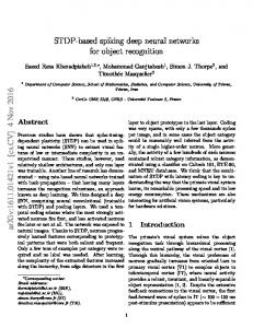
well the classifier will perform on new data. Hence the test error indicates how well your model generalizes to new data. A related concept to generalization is overfitting. Overfitting occurs when the model has learned to fit the noise in the training data, instead of learning the underlying structure of the data. In figure 1.1 the green line represents an overfitted model and the black line

Figure 1.1: Example of overfitting [4]. represents a regularised model. The green line best follows the training data, and it is likely to have a higher test error, compared to the black line. Overfitting manifests itself when a model is more flexible than it needs to be or includes irrelevant components [20]. Underfitting on the contrary, arises when the model has not learned the structure of the data.

1.2

Computer Vision

Computer vision is a subfield of Artificial Intelligence which aims at the analysis and interpretation of visual information. Image understanding is considered as a process starting from an image or from image sequences and resulting in a computer-internal description of the scene [21]. Human beings and animals have the innate capability of take decisions on what they see, providing such a visual understanding to computers

1. Background

8

would allow them the same power. The approach to CV can be decomposed in three main processing components: • Image acquisition: is the process of translating the analog world around us into digital representations. • Image processing: applies algorithms to the digital data acquired in the first step to infer low-level information on parts of the image (includes methods to handle processing problems such as noise reduction and signal restoration). • Image analysis and understanding: high-level algorithms are applied to both the image data and the low-level information which are computed in the previous steps. Computer vision is closely related to a number of fields. For instance, because it elaborates image data, many methods are shared with the Image Processing and more generally with Signal Processing research fields. Computer vision algorithms make use of mathematical and engineering fields such as Geometry, Optimization, Probability Theory, Statistics, etc. [22]. Computer vision has several applications in different domains. Indeed, the use of a vision sense is not limited simply to robotics, other examples are medical research, military applications and space explorations. Each of the domains mentioned above employs a range of computer vision tasks. Some examples of typical computer vision tasks are presented below: • Recognition: aims to decide whether or not the image data contains some specific element (object, activity, etc.). • Motion analysis: aims to analyze the motion of an element in a sequence of images. • Scene reconstruction: tries to reconstruct a 3-Dimensional model from more images of a specific scene.

1. Background

9

• Image restoration: executes the removal of noise (sensor noise, motion blur, etc.) from images. According to the context of this dissertation, in the following sub-sections, a brief introduction to image processing, and its operation of segmentation, is provided. Moreover, the recognition’s task and the applications of computer vision to Robotics are discussed in detail.

1.2.1

Image Processing

The acquisition of a digital image is a two-dimensional representation of a threedimensional visual world. Sometimes the captured images are noisy or degraded. For instance, we receive blurred images if the camera is not appropriately focused or the scene is captured outdoor in foggy conditions. In this case, image processing’s techniques aim to refine the images so that the resultant images are of better visual quality, free from noise. In general terms, image processing is processing of images using mathematical operations by using any form of signal processing for which the input is an image, a series of images or a video, such as a photograph or video frame; the output of image processing may be either an image or a set of characteristics or parameters related to the image [23]. Among many other, common image processing operations are[24]: • Euclidean geometry transformations such as enlargement, reduction, and rotation • Color corrections such as brightness and contrast adjustments, color mapping, color balancing, quantization, or color translation to a different color space • Image differencing and morphing • Interpolation, demosaicing, and recovery of a full image from a raw image format using a Bayer filter pattern • Image segmentation • High dynamic range imaging by combining multiple images

1. Background

10

Image Segmentation In this context, image segmentation is the process of partitioning a digital image into multiple regions (segments) of related contents. Each of the pixels in a segment are similar with respect to some characteristic, such as gray tone or texture. Image segmentation is an important step from the image processing to image analysis because it affects the feature measurement helping high-level image analysis and understanding. According to [25], image segmentation methods can be classified in layer-based and blockbased. Layer-based methods are used for object detection and image segmentation that relies on the output of several object detectors. This class of techniques are of less interest for this dissertation. Block-Based methods are based on various features found in the image such as color or information about the pixels that indicate edges, boundaries, texture. This class of methods can be sub-divided in: • Region-based methods: aim to segment the entire image into sub regions or clusters, for example on the basis of the gray color level in one region. • Edge or boundary based methods: transform images to edge images using changes of gray tones in the images. Edges are important because signalize the lack of continuity and occur on the boundary between two regions. Within region-based class methods, thresholding is the simplest image segmentation method. Starting from a grayscale image, thresholding can be used to separate foreground (region of interest) from the background. The simplest thresholding method converts grayscale images to binary images by selecting a single threshold value. Other thresholding methods are the following: • Histogram Dependent: selects the threshold value by analyzing image histograms which can be one of two models: Bimodal and Multimodal. In the former, histograms present two peaks and a clear valley where threshold is the valley point. The latter presents a more complex threshold selection because there are many peaks and not a clear valley.

1. Background

11

• P-Tile: uses knowledge about the area size of the object, based on the gray level histogram, assumes the objects are brighter than the background and occupy a fixed percentage. • Edge Maximization: depends on the maximum edge and edge detection techniques. • Local: adapts the threshold value on each pixel to the local image characteristics. In these methods, a different threshold is selected for each pixel in the image. • Mean:uses the mean value of the pixels as threshold value.

1.2.2

Object Recognition

In computer vision, object recognition is a subclass of the Recognition problem. The aim of object recognition is to process images or video sequences in order to identify and classify objects. This task represents a complex challenge for computer vision systems. In fact, object recognition involves segmentation, dealing with variations in lighting, viewpoint and occlusions (parts of an object can be hidden behind other objects).

Figure 1.2: Object recognition as labeling problem [5]. As shown in Figure 1.2, Object recognition can be defined as a labeling problem. Formally, first the system receives an image containing one or more objects of interest

1. Background

12

and a set of labels, then it assigns the correct labels to regions, or a set of regions, in the image. In the last decades, several algorithms and model have been used to achieve object recognition such as SIFT (Scale-Invariant Feature Transform), SURF (Speeded-Up Robust Features), LDA (Linear Discriminant Analysis) and CNN (Convolutional Neural Network). Most of the above mentioned algorithms, for instance SIFT, are hand-crafted and require a certain amount of engineering behind them. These techniques are known as shallow, where the learning is done only at mid-level by training classifiers such as Support Vector Machines (SVM), Random Forest or Naive Bayes classifier [26]. On the other hand, CNNs have become in the last few years the state-of-the-art for a variety of large-scale pattern recognition problems [27], among which Object Recognition. Convolutional Neural Networks are introduced in chapter 2 .

1.2.3

Robotic Applications

Computer vision algorithms are widely used in Robotics. As an example, personal robotics is an exciting research frontier with a range of potential applications including domestic housekeeping, caring of the sick and the elderly, and office assistants for boosting work productivity. In this context, the ability to detect and identify objects in the environment is fundamental. Robot vision involves using a combination of camera hardware and computer vision algorithms to allow robots to process visual data from the world. Unlike pure computer vision research, robot vision must incorporate aspects of robotics into its techniques and algorithms, for instance visual servoing consists in controlling the motion of a robot by using the feedback of the robot’s position as detected by a vision sensor. Nowadays, providing robots with accurate and robust visual recognition capabilities in the real-world is a challenge which obstacles the use of autonomous agents for concrete applications. In fact, the majority of tasks, as manipulation and interaction with other agents, severely depends on the ability to visually recognize the entities involved in a scene. Object recognition represents a complex challenge for robotic vision systems because

1. Background

13

the real-world setting differs from the typical retrieval scenario. In robotic systems, the ability to learn incrementally, in a human-like fashion, new classes of objects is highly desirable. This problem of learning from a continuous stream or a block of new images is known as Incremental Learning. The nature of the learning problem is affected by the amount and type of visual data, this means that datasets must present specific properties according to the specific task, as an example datasets for incremental learning are made of few video frames rather than millions of independent images. In the last years, many vision systems have been ultimately tested on datasets tailored to image retrieval problems while only few datasets and benchmarks suitable for robotic object recognition have been made available.

1.3

Artificial Neural Networks

In machine learning, Artificial Neuron Networks (ANNs) are a computational model based on the structure and functions of biological neural networks which are common in the brains of many mammals. Figure 1.3 illustrates the analogies between a biological neuron and an artificial neuron unit.

Figure 1.3: A biological neuron and the relative inspired mathematical model[6]. As we can see, a biological neuron consists of a cell body, a collection of dendrites and an axon. Dendrites bring electrochemical information into the cell, from external

1. Background

14

impulses. If these impulses reach a certain threshold, the axon fires electrochemical information out of the cell. The axon from one neuron can influence the dendrites of another neuron across junctions called synapses. The artificial neural unit is a mathematical model of the biological neuron behavior and structure. Dendrites are formalized as the multiplication w0 x0 between the axon x0 , and the synapse w0 (input weight of the neuron). The dendrites carry out the signals w0 x0 to the cell body where all the inputs plus a bias b are summed. If the final sum exceeds a certain threshold, the neuron fires. This firing strength is modeled by the activation function f . Commonly used activation functions are the sigmoid, tanh and rectifier. An ANN can dynamically learn to change its weights and bias, in order to control the strength of influence of one neuron on another.

1.3.1

Feedforward Neural Network architecture

A Feedforward Neural Networks is the simplest type of ANN: the information moves in only one direction, forward, from the input neurons, through the hidden neurons (if they exist) and to the output neurons. Thus, in this network the connections between units do not form a cycle. Instead of an amorphous set of connected neurons, neural network models are often organized into distinct layers of neurons. Figure 1.4 illustrates a simple 3-layer Feedforward Neural Network architecture with two hidden layers.

Figure 1.4: A 3-layer Feedforward Neural Network architecture [6].

1. Background

15

Hidden layers are a set of neurons connected to other layers of neurons, therefore they are not visible as a network output (this explains the term hidden layer). Hidden layers are important because they can find features within the data and allow following layers to operate on those features rather than the noisy and large raw data. The typical layer type is the fully-connected layer in which neurons between two adjacent layers are fully connected pairwise. Neurons in a single layer do not share any connections. Even though, feedforward networks is a simple ANN model, it has been proved that multilayer feedforward networks are a class of universal approximators [28]. This result establishes that for every possible function, f , and input, x, exists a standard multilayer feedforward networks with as few as one hidden layer able to return, as output from the network, the value f(x) (or some close approximation).

1.3.2

Backpropagation algorithm

Backpropagation (BP) is an efficient method of computing gradients in directed graphs of computations, such as neural networks. BP provides detailed insights into how changing the weights and biases changes the overall behaviour of the network. At the hearth of BP is an expression for the partial derivative ∂C/∂w of the cost function C with respect to any weight w (or bias b) in the network. During the training phase, an ANN learn how to change the weights w and b in order to minimize C that represents the distance from the goal of the training. Let N be a feedforward neural network with e connections, where x, x1 , x2 , . . . , xj ∈ Rn are the input vectors, w, w1 , w2 , . . . , wt ∈ Re are the weights vectors, y, y1 , y2 , . . . , yj ∈ Rn are the output vectors. We can define the neural network as a function: y = fN (w, x) The above function, given a weight w vector maps an input x to an output y. Let y´ be our target correct output, we can use an error function E in order to measure the difference between the two outputs. A common choice is the the square of the Euclidean distance: E(y, y´) = |y − y´|2

1. Background

16

During the training phase, the backpropagation algorithm takes as input a sequence of training examples (x1 , y1 ), (x2 , y2 ) . . . , (xj , yj) and produces a sequence of weights vector w0 , w1 , . . . , wj which starts with some initial random weight w0 . The goal of the backpropagation algorithm is to find the weights that best minimize the error function E. The backpropagation algorithm can be divided into two phases: 1. Forward pass: computes for each (x0 , w0 ) . . . , (xj , wj) the output activation y0 . . . yj and the relative training error E(y, y´). 2. Backward pass computes the wi using only (xi , yi , wi−1 ) for i = 1, . . . , p. The weight vector wi is produced applying gradient descent to the function wi−1 → E(fN (wi−1 , xi ), yi ) to find a local minimum. The error is propagated backward starting from the output layer, through the hidden layers, to the input layer. Hence, wi is the minimizing weight vector found by gradient descent with some update rule. It’s worth noting that the weight update difference, from wi−1 to wi , is proportional to the negative of the gradient at the current point (in the network) and the value of the learning rate. The learning rate multiplies the gradient of a weight before the updating, therefore the greater the value, the faster the neuron trains, but the lower the value, the more accurate the training performs. The sign of the gradient of a weight points out where the error is increasing, this explains why the weight must be updated in the opposite direction.

1.4

Deep Learning

Deep learning (DL) is a collection of machine learning algorithms that use a specific approach for building and training neural networks. Deep learning algorithms model high-level abstractions in data by using ANNs with multiple processing layers, composed of multiple linear and non-linear transformations [27]. DL is part of a broader family of machine learning methods based on learning data representations which replaces the more difficult manual feature engineering. Many different architectures such as convolutional deep neural networks, deep belief networks

1. Background

17

and recurrent neural networks have proved to achieve state-of-the-art results on various tasks of computer vision, natural language processing, automatic speech recognition and bioinformatics. Over the years, the path towards deep learning models has faced several challenges and limitations, such as slowness of computations and problems related to the gradient descent strategy. For instance, traditional deep feedforward or recurrent networks suffer from the famous problem of vanishing or exploding gradients [29]. In basic terms, backpropagation relies on backpropagating the error from the output to prior layers. Networks with many layers, lead to a long sequence of calculus-based computations which produce either huge or tiny numbers. In this scenario the resulting neural net is not able to update significantly or correctly prior layers weights, thus it is not learning at all. The following findings are some of the main discoveries that have contributed to overcome the problems related to deep neural networks: • Parallel computation: parallel computing power of GPUs over CPUs leads to much faster training phase. • Rectified linear activation function: leads to sparse representations, meaning significant computational efficiency. The simplicity of this function, and its derivatives, makes it much faster to work with than the sigmoid activation function. Rectified Linear Unit saturates only when the input is less than 0, avoiding meaningless backward pass when the derivative is very close to 0. • Weight initialization: backpropagation converges to different optimal points for different initial conditions. So it not only affects the speed of the convergence but optimality. Thus, it is important to use efficient common initialization techniques such as normalized Gaussians.

Chapter 2 CNN for Object Recogntion “The key to artificial intelligence has always been the representation.” - Jeff Hawkins, On Intelligence (2004) The current chapter describes the Convolutional Neural Network (CNN) learning model in the context of object recognition. In the following sections we provide an introduction to the basic concept of convolution, an overview of the CNN model and details about its layers, architecture and learned features.

2.1

Digital images and convolution operations

A digital image is a numeric representation of a two-dimensional real image. There are two main type of digital images: vector and raster. Vector graphics describes the primitive elements, which compose the image, through the use of vectors. On the other hand, raster graphics describes a real image with a matrix of points, called pixels. One or more digital values define the color of pixels. Raster images are also referred as bitmap images. An image can be stored as a two-dimensional (matrix) or three-dimensional data structure depending on whether it is a coloured bitmap or grayscale bitmap. For instance, in the RGB model, the color is represented as level of intensity of three basic 18

2. CNN for Object Recogntion

19

Figure 2.1: A coloured bitmap mapped as three-dimensional data structure colors: red, green and blue. Figure 2.1 illustrates a RGB bitmap mapped as threedimensional structure where each matrix maps the information about the intensity of the relative color. In grayscale bitmaps, for each pixel one numeric value is enough to indicate the different gray intensities ranging from black to white, therefore just one matrix is needed. A bitmap is characterized by the width and height of the image in pixels and by the number of bits per pixel. As an example with 8-bit per pixels is possible to represent 256 gray levels. Depending on the compression algorithm, generally lossy or lossless, bitmap images can be stored in different formats. Convolution is a mathematical operation which is fundamental to many common image processing operators. Convolution provides a way of ”multiplying together” two arrays of numbers, generally of different sizes, but of the same dimensionality, to produce a third array of numbers of the same dimensionality [30]. In image processing, one of the input arrays is normally a grayscale image, while the second array is a smaller matrix known as convolution matrix, filter or kernel. In this context an operator that implements convolution produces an output image as simple linear combinations of the input pixel values. A filter can be thought as a sliding window moving, from left to right and from top to bottom, across the original image. Generally the filter moves through all the positions where it fits entirely within the boundaries of the image. At each shift, the filter produces a single output pixel, whose value is calculated by summing all the products between


20

the filter elements and the corresponding pixels.

Figure 2.2: A single step of convolution performed on 9 × 9 image and a 3 × 3 kernel. Figure 2.2 shows the output produced from a 3 × 3 filter at the center of 9 × 9 image. The resulting image highlights the characteristics enhanced by the filter used. As a result, in computer vision, several filters are used for different purposes. The more popular are: • Gaussian filters: normally used to remove noise by taking average between the current pixel and a specific number of neighbours. • High-pass filters: normally used to improve image details. • Emboss filters: normally used to enhance brightness differences. • Sobel filters: normally used to highlight edges. Until now, we have only discussed one to one convolutions that apply a filter to single image. We can identify other two kinds of convolution: • One to many convolution: when there are n filters and only one input image. In this case, each filter is used to generate a new image. • Many to many convolution: when there is n filters and more than one input image. Each connection in between input and output images is characterized with specific different filters.


2.2

21

Convolutional Neural Network: an overview

Convolutional Neural Networks (CNNs) are a category of Feedforward Neural Networks. Likewise, CNNs are made up of neurons with learnable weights and biases. Again, backpropagation is the algorithm used for training the network. Historically, CNNs have been used in the context of image classification, indeed the typical CNN input is a multi-channeled image. In the last decades, the neuroscience community has proved that one of the unique ability of the human visual system is called perceptual invariance and it emerges from the complex (and generally hierarchical) organization of connections in the brain. This and other studies, have directly inspired the architecture of CNNs. The CNN multi-layer architecture resembles the organization of information in the human visual system in order to achieve robustness against shifting, distortion and scaling of objects. Deep neural networks composed by only fully connected layers involve a huge number of parameters which would most likely lead to overfitting or it can just be wasteful in terms computation. Therefore, CNNs use convolutional layers which rely on ideas like local receptive fields and shared weights. Normally convolutional layers execute many to many convolutions. Each neuron of the layer performs a convolution where its weights are the values of the filter. Convolution layers involve a smaller number of weights respect fully connected layers. For example, when processing an image, the input image might have thousands or millions of pixels, but we can detect small, meaningful features such as edges with kernels that occupy only tens or hundreds of pixels [31]. This means that we need to store fewer parameters, which both reduces the memory requirements of the model and improves its statistical efficiency. In brief, CNNs differ from other ANN models in that they are composed of a particular set of layers, such as convolutional layers or downsampling layers, which are inserted in a specific sequence.


2.3

22

Layers used to build CNN

One of the key characteristics of CNN is the particular set of layers which composes the network. In literature, it is possible to identify three main kinds of layers which are described in the following sub-sections.

2.3.1

Convolutional layer

The first layer in a CNN is always a convolutional layer. In a convolutional layer only small localized regions of the input are connected to every hidden neuron. That region in the input image is called the local receptive field for the hidden neuron. Figure 2.3 shows a 5 × 5 local receptive field which corresponds a filter of the same size. The filter numeric values represent the weights of the hidden neuron. Likewise convolutions in computer vision, each filter convolves over all the locations of the input image, producing an output image called activation map.

Figure 2.3: A 5 × 5 filter convolving an input volume and producing an activation map [7]. It is worth noting that, the extent of the connectivity along the depth axis of the local receptive field is always equal to the depth of the input volume. For example, if the receptive field is 5 × 5 and the input image is [32 × 32 × 3], then each neuron will


23

have weights to a [5 × 5 × 3] region in the input volume. Moreover, convolutional layers implement parameter sharing. Basically, parameter sharing constrains the neurons to use the same weights and bias. Thus, because the filter is shared, all the neurons in the convolutional layer detect exactly the same feature, just at different locations in the input image. Informally, a feature is a type of input pattern (an edge in the image) that will cause the neuron to activate. For this reason, the activation map is also called feature map. The number of feature maps corresponds to the depth (third dimension) of the convolution output volume. The importance of detecting different image features explains why a convolutional layer produces several feature maps. In fact, generally, a convolutional layer increase the dimensionality of the input volume on the depth axis (third dimension). A real world example is the Krizhevsky architecture [2] that won the ImageNet challenge in 2012. Figure 2.4 shows 90 of the 96 filters learned by Krizhevsky at the first convolutional layer. The size of each filters is [11 × 11 × 3], and each one is shared by the 55 ∗ 55 neurons in one feature map.

Figure 2.4: Example filters learned by Krizhevsky [2]. In general the output volume is controlled by three hyperparameters: • Depth: this parameter sets the amount of filter used equivalent to the amount of feature map produced.


24

• Stride: this parameter controls how we slide the filter. For instance, when the stride is 1, the filter moves one pixel at time. • Zero-padding: if greater than zero, this parameter pads the input volume around the border with a number of zeros according to the specified value. The following formula can be used to find the size (first two dimensions) of the output volume: (W − F + 2P )/S + 1 where W is the input volume size, F represents the filter size of the convolutional layer, S and P are the stride and the amount of zero padding respectively.

2.3.2

ReLU Layer

Generally, after each convolutional layer, it is convention to apply a ReLU (Rectified Linear Units) layer (or activation layer). The ReLU layer applies the rectifier activation function: f (x) = max(0, x) to all of the values in the input volume. Practically speaking, this layer just changes all the negative activations to 0. As mentioned in chapter 1, there are other activation functions like tanh and sigmoid. In the last decade, Researchers have found out that ReLU layers work far better [32] because the network is able to train a lot faster without making a significant difference to the accuracy. Additionally, it helps to alleviate the vanishing gradient problem.

2.3.3

Pooling layer

A Pooling layer applies a form of non-linear downsampling. The aim of downsampling is to reduce the spatial size of the representation. In this category maxpooling layer are the most popular. This pooling layer uses the MAX operation on a subregion of the input (filter), normally of size 2 × 2, with a stride of the same length. Hence, it outputs


25

Figure 2.5: Example of maxpooling with a 2 × 2 filter and stride 2 [6]. the maximum number in every subregion that the filter convolves around. For threedimensional input, every depth slice is downsampled along both width and height. In figure 2.5, the output of maxpooling layer with a 2 × 2 filter and stride 2 is shown. There are two main benefits from using pooling layers in CNN: 1. The number of parameters is drastically decreased, thus lessening the computation cost. 2. The threat of overfitting is reduced, thus the network’s ability of generalization is improved. As an aside, some CNNs use 1x1 convolutions as a feature pooling technique. For example, an image of 150 × 150 with 30 features on convolution with 10 filters of 1 × 1 would result in size of 150 × 150 × 10. In this context, 1 × 1 convolution can be useful because we operate on 3-dimensional volume, although, on two dimensional input, it would be pointless.

2.3.4

Fully connected layer

In chapter 1, the fully connected layer it has been introduced as the typical layer of an ANN. In a CNN they are normally used for learning non-linear combinations of high level


26

features. Essentially, the aim of convolutional layers is to provide an invariant feature space, and the aim of fully-connected layer is learning a function (generally non-linear) in that space.

2.4

CNN architecture

In this section we discuss how the layers, described in the previous section, are stacked together to form a CNN. The architecture of a CNN can be divided into three parts, as shown in figure 2.6. First of all, a CNN receives in input a sequence of digital images; then the input is given to a feature extraction module which generates an array of features; finally this array is delivered to a full connected neural network that produces the results.

Figure 2.6: General CNN architecture divided in its fundamental parts The feature extraction module is composed by an alternation of three layer types: CONV(Convolutional), ReLU and POOL (Pooling). The most common architecture follows the pattern: IN P U T → [[CON V → RELU ]] ∗ N → P OOL?] ∗ M where * represents repetition and POOL? an optional Pooling layer. Usually 0 ≤ K ≤ 3 and 0 ≤ N ≤ 3.


27

Instead, the full connected neural network is composed by an alternation of FC (Fully connected ) and RELU layers. It can be described by the following pattern: [F C → RELU ] ∗ K → F C where again 0 ≤ K ≤ 3. Figure 2.7 provides an overview of a typical CNN architecture with 5 layers. All the convolutions are many to many, i.e. each feature map has a neuron that can be connected with two or more feature maps of the previous layer.

Figure 2.7: A simple CNN architecture [8] In this section we have discussed the typical CNN architecture, however there many variants depending on the task. For instance, there are CNN without final neural network. In this case other classifier, such as Support Vector Machine, can be used.

2.5

CNN training

The backpropagation algorithm, introduced in the previous chapter, computes (analytically using the chain rule) the gradient of a CNN loss function with respect to its weights. The backpropagation (BP) is used as a gradient computing technique by the gradient descent optimization algorithm. Gradient descent is currently the most common and established way of optimizing CNN loss functions. Training a CNN from scratch with the gradient descent algorithm is not the only strategy. Gradient descent and other CNN training strategies are described in the following subsections.


2.5.1

28

Gradient descent

The procedure of repeatedly evaluating the gradient of a loss function and then performing a parameter update is called gradient descent. This algorithm is widely used to train CNNs. A code implementation of gradient descent looks as follows: 1 f o r i in range ( i t e r a t i o n s ) : 2

weights grad = evaluate gradient ( loss fun , train data , weights )

3

w e i g h t s += − s t e p s i z e ∗ w e i g h t s g r a d

This simple loop is at the core of all Neural Network libraries. Besides, there are some variants of gradient descent, which differ in how much data we use to compute the gradient of the loss function: • Batch gradient descent: it computes the gradient of the cost function with respect to its parameters for the entire training dataset. Thus, we need to calculate the gradients for the whole dataset to perform just one update. It can be very slow and expensive in terms of memory (dataset could not fit in RAM). BGD is guaranteed to converge to the global minimum for convex error surfaces and to a local minimum for non-convex surfaces. • Stochastic gradient descent: it computes the gradient of the cost function with respect to its parameters for one training example at each step. Hence, SGD performs a parameter update for each training example with a high variance that cause the loss function to fluctuate heavily. SGD’s fluctuation allows it to jump to new and potentially better local minima. On the other hand, this ultimately complicates convergence to the exact minimum. SGD is usually much faster than BGD since it updates weights more frequently. • Mini-batch gradient descent: a compromise between BGD and SGD, is to compute the gradient against more than one training example at each step. MGD performs an update for every mini-batch of n training examples. This approach reduces the variance of the parameter updates, which can lead to more stable convergence. Mini-batch gradient descent is typically the algorithm of choice when training ANN. Common mini-batch sizes range between 50 and 256, but can vary for different applications.


29

Even though SGD technically refers to using a single example at a time to evaluate the gradient, the term SGD is employed even when referring to mini-batch gradient descent, where it is usually assumed that mini-batches are used.

2.5.2

Training strategies

When training a CNN from scratch (with random initialization), it is relatively rare to have a dataset of sufficient size. Moreover, training from scratch might take a long time to complete (days, weeks). Instead, it is common to pre-train a deep CNN (base network) on a very large dataset and then use its the weights as an initialization for a second CNN (target network). This scenario is known as Transfer Learning. There are two main strategies, in the context of transfer learning: • Fine-tuning the ConvNet: it consists in copying the first n layers of the trained base network to the first n layers of the target network and in fine-tuning the copied weights of target network by continuing the backpropagation (training). The choice of whether or not to fine-tune the first n layers of the target network depends on the size of the target dataset and the number of parameters in the first n layers [33]. This strategy is motivated by the observation that earlier layers of a ConvNet learn more generic features (e.g. Gabor filters or color blobs) which should be useful to many tasks, instead later layers of the ConvNet are progressively more specific to the details of the classes contained in the original base dataset. When transferred layers are not fine-tuned, copied weights are left frozen, meaning that they don’t change during training on the new task. • ConvNet as fixed feature extractor: as mentioned in section 2.4, the central module of a CNN works as feature extractor. In this strategy, again, layers from the trained base network are copied into the target network. Then, the last fullyconnected layers are removed from the target network, which is treated as fixed feature extractor for a new dataset. For every image in the dataset, a corresponding feature vector is extracted and used to train a linear classifier (e.g. Linear SVM or Softmax classifier).


2.6

30

Visualizing and understanding deep CNN

In the last years there has been considerable improvements in the creation of highperforming architectures and learning algorithms for deep neural networks. On the other hand, the understanding of how these large neural models operate has lagged behind. In fact, it is tough to understand exactly how any trained neural network works due to the huge number of interacting, non-linear parts. This has led to consider neural netowrks as black boxes, especially deep neural networks composed by several layers. According to [34] there are different approaches that try to understand, through features visualization, what is learned at each level of a DNN. One approach is to interpret the function computed by each individual neuron. Past studies in this vein divide into two different camps: dataset-centric and network-centric. Examples from the two classes will be discussed in the following subsections.

2.6.1

Dataset-centric approach

Dataset-centric techniques require both a trained DNN and running data through that network. One famous dataset-centric approach is the deconvolution method [9] which highlights the portions of a particular image that are responsible for the firing of each neural unit (within its feature map) at any layer in the model. This technique is based on a Deconvolutional Network (deconvnet). A deconvnet uses the same components of a convnet (convolutional, pool layers etc.) but in reverse (unpool, rectify, etc.), thus it maps features to pixel. At the beginning an input image is forwarded throughout the convnet, then to examine a given layer activation, one of the relative feature maps is passed as input to the attached deconvnet layer. The deconvnet layer reconstruct the activity in the layer beneath that gave rise to the chosen activation. This is then repeated until input pixel space is reached. Figure 2.8 shows the top nine activations in a random subset of feature maps across the validation data, projected down to pixel space using the deconvolutional network approach in [9].


31

Figure 2.8: Visualization of features in a fully trained model [9]

2.6.2

Network-centric approach

Network-centric techniques require only the trained network itself. Consequently, they investigate directly a DNN without any data from a dataset. In this category, as an example, Simonyan et al. (2013) [10] use the gradient ascent technique, introduced by [35], in order to address the visualization of deep image classification CNNs. The procedure is related to the CNN supervised training procedure, but in this case the optimization is performed with respect to the input image (weights are fixed to those found during the training stage). In basic terms, the objective of the optimization is to maximize the score (neuron response in the final layer) of a given class of images. In the first step (forward pass) of the algorithm, an image with random pixel colors is forwarded throughout the network. Also, it is selected the class score to be maximized. In the second step (backward pass), the gradient of the class score with respect to the input image is performed. The pixel color values are updated adding the product between the


32

gradient result and the learning rate. This two-step process is repeated until satisfying results are achieved.

Figure 2.9: Pictures produced by maximization of three different class scores [10] Figure 2.9 shows three images produced by maximizing a given class score: bell pepper, lemon , husky. The three pictures resemble some recognizable features of the related class models. It was worth mentioning that these results were achieved by employing L2-regularization. In fact, without such a regularization form, would have been harder to recognize class appearance models. The visualization of such images suggest qualitatively which invariant features the network has learned from different classes.

Chapter 3 CORe50 “In God we trust; all others must bring data.” - professor W. Edwards Deming In this chapter, CORe50 a new dataset and benchmark for continuous object recognition, is introduced. In the first section few datasets similar to CORe50 are briefly described. In section two, an overview of CORe50, with details on its design and aim, is provided. Finally, the process for integrating the depth information in CORe50 is illustrated.

3.1

Existing datasets and their limitations

In the context of object recognition, CORe50 is a dataset for incremental learning. Therefore, we present only existing datasets suitable for incremental learning strategies. Most of the datasets described in the following sub-sections have been used by Maltoni and Lomonaco [36] for accuracy evaluation of incremental learning strategies. In particular, we focus on the limitations of such datasets in order to justify the creation of CORe50.

33

3. CORe50

3.1.1

34

iCubWorld28

iCubWorld28 is a significant dataset in the robotics field. It consists of 28 different objects organized into 7 categories. For each object are acquired 220 images (128 × 128 pixels in RGB format) for both train and test set. This acquisition collects one dataset of more than 12K images and runs over four days (4 dataset). Maltoni and Lomonaco [36] reach an averaged accuracy of 75% using the fine-tuning strategy over the CaffeNet network. In the context of Incremental Learning, the main limitations of this dataset are: • the small number of sessions: 4; • the small number of objects: 28; • the maximum resolution of 128 × 128; • the limited background variation: only indoor acquisition

3.1.2

Big Brother

The BigBrother dataset is composed by 23.842 70 × 70 gray-scale images of faces belonging to 19 competitors of famous Italian reality show. The dataset is divided into training set, test set and an additional set of images, called ”updating set “. The updating set is provided for incremental learning/tuning purposes. Again, according to [36], fine-tuning the CaffeNet with a pretrained model is the most effective strategy, even though the best reached averaged accuracy is smaller (of some points) respect the ICubWorld28. The BigBrother dataset has a small number of images compared to the iCubWorld28 dataset. Moreover, it presents only faces and it is not useful for generic object recognition.

3.1.3

NORB dataset

NORB is one of the best dataset to study invariant object recognition. It is composed by 50 uniform-colored objects under 36 azimuths, 9 elevations, and 6 lighting conditions (for a total of 194,400 individual images). The objects are 10 instances of 5 classes. The

3. CORe50

35

image resolution and image format are 640 × 480 and RGB respectively. Furthermore, temporally coherent video sequences can be generated from NORB by randomly walking the 3D variation space. Thus, the NORB dataset contains a significant number of frames and variations. On the other hand, the images recorded are untextured toys without natural background.

3.2

CORe50: an overview

Maltoni and Lomonaco introduce CORe50 [3] as a new dataset and benchmark for continuous object recognition. Being specifically designed for incremental learning strategies, Core50 is well-suited to this purpose. As we have seen in the previous sections, several datasets used for incremental learning lack of fundamental properties. CORe50 consists of 50 domestic objects belonging to 10 classes: markers, plug adapters, balls, mobile phones, scissors, light bulbs, cans, glasses, cups and remote controls (see Figure 3.1)

Figure 3.1: The 50 different objects of CORe50. Each column denotes one of the 10 categories [3]. CORe50 supports classification at object level (50 classes) or at category level (10 classes). The former (the default one) is much more challenging because objects of the same class are very difficult to be distinguished under certain poses. The dataset has

3. CORe50

36

been collected in 11 distinct sessions (8 indoor and 3 outdoor) characterized by different backgrounds and lighting (see Figure 3.1). For each session and for each object, a 15 seconds video (at 20 fps) has been recorded with a Kinect 2.0 sensor delivering 300 RGB-D frames. The presence of temporal coherent sessions (i.e., videos where objects gently move in front of the camera) is another key characteristic since temporal smoothness can be employed to ease object detection, improve classification accuracy and to address semi-supervised (or unsupervised) scenarios. The camera point of view coincides with the operator eyes. Objects are hand hold by the operator, therefore relevant object occlusions are often produced by the hand itself. Moreover, a point-of-view with objects at grab-distance is appropriate for a number of robotic applications. Figure 3.2 depicts one frame of the same object throughout the eleven session. Note the variability in terms of illumination, background, blurring, occlusion, pose and scale.

Figure 3.2: One frame of the same object throughout the 11 acquisition sessions [3].

3.2.1

RGB-D dataset

An important feature of CORe50 is the opportunity to run experiment exploiting the depth information of the images. The Kinect RGB-D cameras provide dense depth estimations together with color images at a high frame rate. During acquisition, the Kinect records 1024 × 575 RGB + 512 × 424 Depth frames. A central region, in the acquisition interface, points out where the object should be kept (see Figure 3.3). This can be used for reducing (cropping) the RGB frame size to 350 × 350. Because only a small fraction of the RGB frame contains the object of interest, it

3. CORe50

37

Figure 3.3: The Acquisition interface [3]. has been exploited temporal information to crop from each 350 × 350 frame a 128 × 128 box around the object. In most cases, the motion-based tracker implemented to this purpose fully contains the objects in the crop window. Nevertheless, sometimes objects can extend beyond border due to tracking imperfections. Moreover, since the motion based tracker is not always able to identify an object in the first frames of a session, less images have been acquired for the cropped dataset. In summary, three dataset have been produced: • CORe50 350x350 rgb: composed by 165,000 350 × 350 images: 11 sessions × 50 objects × 300 frames per session. • CORe50 128x128 rgb: composed by 164,866 128 × 128 images: 11 sessions × 50 objects × ∼ 300 frames per session. • CORe50 512x424 depth: composed by 164,740 512 × 424 images: 11 sessions × 50 objects × ∼ 300 frames per session. Note that also CORe50 512x424 depth presents less images. This is due to the fact that, during acquisition, the Kinect depth sensor was not perfectly synchronized with

3. CORe50

38

the RGB camera. The Kinect 2.0 contains a Time-of-Flight (ToF) camera and determines the depth by measuring the time emitted light takes from the camera to the object and back. Therefore, it constantly emits infrared light with modulated waves and detects the shifted phase of the returning light [37]. In the following, we refer to both cameras (Pattern Projection and ToF) as depth camera. The color and depth camera have different resolutions and are not perfectly aligned, so their view areas differ. Consequently, the color camera covers a wider area than the depth camera. Moreover, elements visible from one camera may not be visible from the other. Figure 3.4 shows an example of the same scene recorded by the color camera (left) and depth camera (right). We will refer to the two images as color frame and depth frame. In particular, the depth frame is a 512 × 424 grayscale image. The scale of grays map the raw depth information (expressed in mm): dark colors represent object closeness. Black pixels indicate portion of the image with no depth information. The color frame is a 350 × 350 cropped RGB image as introduced before.

Figure 3.4: Color frame and corresponding depth frame. In order to correctly exploit the depth information, the depth frame is needed to be mapped to the color frame.

3. CORe50

3.3

39

Integration of the depth information

In light of the two different view areas recorded by color and depth camera, a script for mapping the depth frame to the color frame has been implemented. The integration of the depth information is based on functions within the Kinect for Windows SDK 2.0. The SDK provides tools, APIs both native and managed and support for the features of the Kinect (color images, depth images, audio input, etc.) In particular, the APIs include an handy utility named Coordinate Mapper. CoordinateMapper’s typical job is to identify whether a point from the 3D space corresponds to a point in the color or depth 2D space and vice-versa. It can also be used to directly map 2D locations from the depth frame to color frame and vice-versa. Thus, we have implemented a script in C# that takes in input the CORe50 512x424 depth dataset and produces, for each depth frame, a RGBA frame of the correct mapping (depth to color). The alpha channel has value 0 for all the pixels where no depht information is available, 255 otherwise.

3.3.1

Script details

The algorithm can be divided into four phases. In the following, each phase will be described along with snippets of code. The first phase regards input handling and processing. For each session and for each object, all the depth frames are retrieved. The images are in PNG format, thus they require an appropriate decoding in order to operate on pixels. 1 // FIRST PHASE 2 InitializeComponent () ; 3 sensor = KinectSensor . GetDefault ( ) ; 4 coordinateMapper = s e n s o r . CoordinateMapper ; 5 s e n s o r . Open ( ) ; 6 f o r ( int s = 1 ; s < 1 2 ; s++) 7 { 8

f o r ( int o = 1 ; o < 5 1 ; o++)

9

{

10

f o r ( int i n d e x = 0 ; i n d e x < 3 0 0 ; i n d e x++)

3. CORe50

40

11

{

12

// Open a Stream and decode a Depth PNG image

13

Stream imageStreamSource = new F i l e S t r e a m ( ” . . / c o r e 5 0 5 1 2 x 4 2 4 d e p t h / s ” + s + ” / o ” + o + ” /D ” + f o r m a t I n t ( index , 3 ) + ” . png” , FileMode . Open , F i l e A c c e s s . Read , F i l e S h a r e . Read ) ;

14

PngBitmapDecoder d e c o d e r = new PngBitmapDecoder ( imageStreamSource , BitmapCreateOptions . P r e s e r v e P i x e l F o r m a t , BitmapCacheOption . D e f a u l t ) ;

15

bitmapSourceDepthFrame = d e c o d e r . Frames [ 0 ] ;

16

byte [ ] depthImageArray = new byte [ depthFrameDim ] ;

17

int s t r i d e = ( int ) bitmapSourceDepthFrame . PixelWidth ∗ ( bitmapSourceDepthFrame . Format . B i t s P e r P i x e l / 8 ) ;

18

bitmapSourceDepthFrame . Co pyPi xels ( depthImageArray , s t r i d e , 0 ) ;

19

// G r a y S c a l i n g depth Frame i n i n p u t

20

bitmapSourceDepthFrameGrayScale = GetBmpSourceFromByteArray ( depthImageArray , 5 1 2 , 4 2 4 , 1 ) ;

In the second phase, the depth frame is transformed into an array of ushort and passed as input to the function MapColorFrameToDepthSpace(), method of the Coordinate Mapper class. This function takes in input the 512 × 424 depth frame (as an array of ushort) and return an array of 1920 × 1080 (color frame max resolution) DepthSpacePoints. Depth space is the term used to describe a 2D location on the depth frame. A DepthSpacePoint is composed by two coordinates, X and Y. They specify a row/column location of a pixel where X is the column and Y is the row. So X = 0, Y = 0 corresponds to the top left corner of the image and X = 511, Y = 423 (width-1, height-1) is the bottom right corner of the image. The output array maps for each pixel of the color frame (1920×1080) a DepthSpacePoint that indicates the position on the depth frame (Depth Space). 1 // SECOND PHASE 2 ushort [ ] depthArray = P r o c e s s i n g A r r a y ( depthImageArray ) ; 3 if ( processing ){ 4

d e p t h S p a c e P o i n t s = new DepthSpacePoint [ kinectColorImageDim ] ;

5

coordinateMapper . MapColorFrameToDepthSpace ( depthArray ,

3. CORe50

41

depthSpacePoints ) ; 6 }

In the third phase, the MappingDepthToColorFrame with DepthSP() function is called in order to map the depth information to the color frame. This method iterates on all the DepthSpacePoints of the output array from the previous phase. If a DepthSpacePoint maps to a valid point in Depth Space, an RGBA pixel expressing the depth information in scale of grays is assigned to a 1920 × 1080 mapping image array (original resolution of the color image). Again, depth information is represented with a scale of grays where closeness is expressed with light colors (dark colors otherwise). The if condition at the lines 10/11 checks that depth pixel coordinates are not negative infinity which represent unknown values of depth. In this case the Kinect depth camera could not record depth information due to infrared shadow or noise in the signal. 1 // THIRD PHASE 2 public byte [ ] MappingDepthToColorFrame with DepthSP ( DepthSpacePoint [ ] d e p t h s p a c e P o i n t s , byte [ ] depthImageArray ) { 3

byte [ ] mappingImageArray = new byte [ kinectColorImageDim ∗ 4 ] ; // 1920 x1080 ∗ 4 (RGB−A)

4

// Loop o v e r each row and column o f t h e c o l o r image

5

f o r ( int c o l o r I n d e x = 0 ; c o l o r I n d e x < kinectColorImageDim ∗ 4 ; c o l o r I n d e x=c o l o r I n d e x +4){

6

f l o a t colorMappedToDepthX = d e p t h s p a c e P o i n t s [ c o l o r I n d e x / 4 ] .X;

7

f l o a t colorMappedToDepthY = d e p t h s p a c e P o i n t s [ c o l o r I n d e x / 4 ] .Y;

8 9

// The s e n t i n e l v a l u e i s −i n f , −i n f , meaning t h a t no depth p i x e l corresponds to t h i s c o l o r p i x e l .

10

i f ( ! f l o a t . I s N e g a t i v e I n f i n i t y ( colorMappedToDepthX ) &&

11

! f l o a t . I s N e g a t i v e I n f i n i t y ( colorMappedToDepthY ) ) {

12

// Make s u r e t h e depth p i x e l maps t o a v a l i d p o i n t i n Depth s p a c e

13

int depthX = ( int ) ( colorMappedToDepthX + 0 . 5 f ) ;

14

int depthY = ( int ) ( colorMappedToDepthY + 0 . 5 f ) ;

15

// Are c o o r d i n a t e s i n s i d e t h e 512 x424 Depth Frame?

16

i f ( ( depthX >= 0 ) && ( depthX = 0 ) && ( depthY T white(x, y), otherwise

4. Strategies for preprocessing depth in CORe50

46

where black(x,y) and in white(x,y) are two methods that color a pixel in black and white respectively. The thresholding methods tested in this work can be categorized in three classes: static thresholding (or global thresholding), dynamic thresholding, hybrid thresholding. In static thresholding the threshold value T is specified before the computation for all the dataset images, while in dynamic thresholding for each image of the dataset a specific threshold value is calculated. Hybrid thresholding first executes a static thresholding and then tries to perform a dynamic thresholding. In figure 4.1, it is shown a 128 × 128 mapping frame and its histogram. Note that pixels with zero in the alpha channel are expressed with the black color. The portion of mapping frame with no depth information will be referred as black portion.

Figure 4.1: A 128 × 128 mapping frame and its histogram Most of the mapping frames present histograms with three peaks like the one in the figure above (from left to right): black portion peak, background peak and foreground peak. Peaks and valleys of the image histogram can help in picking the appropriate value for the threshold. Generally, some factors affects the suitability of the histogram for guiding the choice of the threshold: • the separation between peaks; • the noise content in the image; • the relative size of objects (foreground) and background; Dynamic thresholding has been the first tested approach. The Otsu’s Binarization [38] is used to find an ad hoc threshold value for each image in input. The Otsu’s Bina-


47

rization automatically calculates a threshold value from image histogram for a bimodal image (bimodal image is an image whose histogram has two peaks). For images which are not bimodal, Otsu’s Binarization won’t be accurate images. Even though the black portion peak is cleared away (assigned to the background peak) and the image noise is removed, the Otsu’s Binarization fails to find an acceptable threshold value for several images (values too low). A function for finding exactly two peaks from the histogram of an image has been employed over the whole dataset. The table below shows the success rate for each of the dataset sessions.

Session Success rate in finding two peaks

Percentage of the black portion

1

71.05

10.02 %

2

76.40

9.94 %

3

67.24

4.46 %

4

0.17

36.80 %

5

7.17

20.51 %

6

30.48

12.07 %

7

73.48

5.56 %

8

88.53

15.74 %

9

80.10

8.15 %

10

0.45

42.04 %

11

0.68

32.49 %

Table 4.1: Success rate in finding two peaks and percentage of the black portion. By looking at the success rate of session 4 (outdoor),5 (indoor),10 (outdoor) and 11 (outdoor), we understand why the Otsu’s binarization doesn’t perform well. To note that the Otsu’s binarization uses a different algorithm for finding two peaks, therefore it could outperform the table’s results. Furthermore, we have calculated the percentage of the black portion over the eleven sessions, as shown in the third column of the table above. Again results diverge significantly for session 4, 5, 10 and 11.


48

The histogram in figure 4.2 belongs to an object from session 4. Most of the objects’ histograms from outdoor sessions present noise, an high percentage of black portion, several short peaks and an unbalanced relative size of foreground and background.

Figure 4.2: Typical histogram of objects recorded in outdoor sessions In summary, an accurate dynamic thresholding is quite tough to perform due to the complexity and heterogeneity of the dataset. On the other hand, static thresholding guarantees a certain segmentation quality over the whole dataset. For instance, the Otsu’s Binarization finds, for several images, low threshold values which range from 30 to 70. Consequently, most of the background will not be removed but considered foreground (object’s region of interest). The static thresholding approach has been implemented with a global threshold value of 216 which corresponds approximately to 1300 millimeters. As expected, the resulting segmentation masks have demonstrated to be significantly more accurate for outdoor sessions and to present more background noise in the indoor sessions. This has led to conceive and implement the hybrid thresholding. Indeed the hybrid thresholding first executes a static thresholding with a global threshold value of 209 and then performs a dynamic thresholding to achieve a more accurate segmentation. Note that before performing the second dynamic thresholding, foreground pixels are left unchanged (not colored in black). Then we identify relevant peaks from the foreground histogram, according to some specific constrains. Finally a weighted average of the selected peaks is performed in order to assess the dynamic threshold value. Finally, two 128 × 128 segmentation mask’s datasets have been produced: one with the static thresholding approach and the other one with hybrid thresholding approach. After


49

thresholding, morphological operations of dilation have been performed on both datasets.

Figure 4.3: Static thresholding (center) and relative dilation operation (right). Indeed, some object classes, among which scissors and glasses, require operations of dilation. Unfortunately, for these object classes, the recorded depth information is fragmentary, noisy and inaccurate due to limitations of the Kinect depth recording system. Dilation is a morphological operator that gradually enlarge the boundaries of regions of foreground pixels (black pixels in this case). Figure 4.3 demonstrates that dilation improves the segmentation accuracy, incorporating important foreground pixels. On the negative side, dilation adds background noise. A good compromise was achieved iterating dilation operations only on particular objects classes (glasses, scissors, mobile phones) of the training set. Figure 4.4 and 4.5 illustrate a comparison between the segmentation maps produced with hybrid (left) and static (right) thresholding.

Figure 4.4: Hybrid (left) thresholding outperform static (right) thresholding.


50

In the first one, the hybrid approach segments well the image foreground (hand hold object). Instead the static approach considers most of the background as foreground. Conversely, figure 4.5 shows that static thresholding is more accurate (it segments better the object shape), although it adds some background noise.

Figure 4.5: Static (right) thresholding outperform hybrid (left) thresholding. In conclusion two segmentation datasets have been produced: • CORe50 128x128 Mask hybrid: composed by 164,606 128 × 128 grayscale images • CORe50 128x128 Mask static: composed by 164,606 128 × 128 grayscale images The segmentation procedure for CORe50 is not straight due to the high variance of the depth information. The Kinect depth recording system is the main responsible of such complexity. Indeed we have identified issues only during the segmentation of particular sessions or object classes. Either the static and the hybrid approach seem valid solutions (each one has pros and cons), thus we have decided to run experiments on both, in order to understand which one is the best.

4.1.2

Background fading

In the background fading phase, the segmentation mask is used to identify foreground pixels and background pixels. Then, each background pixel is faded to a mean image


51

pixel (gray color) on the basis of its pixel distance to the nearest foreground pixel. The python script that implements the background fading phase is shown below. 1 # Initialization 2 mask main folder path = ’ . . / core50 128x128 Mask hybridApproach / s ’ 3 m a i n f o l d e r d s t p a t h = ’ . . / c o r e5 0 1 2 8 x 1 2 8 b a c k g r o u n d R e m o v e d h y b r i d / s ’ 4 color main folder path = ’ . . / core50 128x128 / s ’ 5 mask img path = ’ ’ 6 color img path = ’ ’ 7 dest img path = ’ ’ 8 s e s s i o n s = 12 9 o b j e c t s = 51 10 i m g s i z e = 1 2 8 . 0 ∗ 1 2 8 . 0 11 mean img = np . z e r o s ( ( 1 2 8 , 1 2 8 , 3 ) , np . u i n t 8 ) 12 # gray c o l o r 13 mean img [ : , : , 0 ] = 104 14 mean img [ : , : , 1 ] = 117 15 mean img [ : , : , 2 ] = 123 16 17 f o r s e s s in range ( 7 , s e s s i o n s ) : 18

o s . mkdir ( m a i n f o l d e r d s t p a t h + ”%s / ” % ( s e s s ) )

19

f o r o b j in range ( 1 , o b j e c t s ) :

20

o s . mkdir ( m a i n f o l d e r d s t p a t h + ”%s / o%s / ” % ( s e s s , o b j ) )

21

mask path = m a s k m a i n f o l d e r p a t h + ”%s / o%s / ” % ( s e s s , o b j )

22

c o l o r p a t h = c o l o r m a i n f o l d e r p a t h + ”%s / o%s / ” % ( s e s s , o b j )

23

f o l d e r s i z e = len ( o s . walk ( mask path ) . next ( ) [ 2 ] )

24

f i r s t f i l e p a t h = Path ( mask path + ”D %02d %02d %03d . png” % ( s e s s , obj , 0 ) )

25

start = 0

26

while not f i r s t f i l e p a t h . i s f i l e ( ) :

27

start = start + 1

28

f i r s t f i l e p a t h = Path ( mask path + ”D %02d %02d %03d . png” % ( s e s s ,

29

folder size = folder size + start

obj , s t a r t ) ) 30 31 32

f o r i in xrange ( f o l d e r s i z e ) : mask img path = mask path + ”D %02d %02d %03d . png” % ( s e s s , obj , i)

4. Strategies for preprocessing depth in CORe50 33

52

c o l o r i m g p a t h = c o l o r p a t h + ”C %02d %02d %03d . png” % ( s e s s , obj , i )

34

# l o a d image i n g r a y s c a l e

35

mask = cv2 . imread ( mask img path , 0 )

36

## l o a d i n BGR format , unchanged

37

c o l o r i m g = cv2 . imread ( c o l o r i m g p a t h , −1)

38

# i f t h e r e i s n ’ t any image jump i t e r a t i o n

39

i f ( mask i s None ) :

40

continue

41

# g e t d i s t a n c e from f o r e g r o u n d p i x e l s

42

d i s t = cv2 . d i s t a n c e T r a n s f o r m ( mask , cv2 . DIST L2 ,

43

max = np .max( d i s t )

44

g = d i s t / (max / 4 )

45

g [ d i s t > max / 4 ] = 1 # f u l l gray p o i n t s

46

g3 = cv2 . merge ( ( g , g , g ) )

47

# output image

48

r e s u l t = c o l o r i m g ∗ ( 1 − g3 ) + mean img ∗ g3

49

d e s t i m g p a t h = m a i n f o l d e r d s t p a t h + ”%s / o%s / ” % ( s e s s , o b j ) +

50

cv2 . i m w r i t e ( d e s t i m g p a t h , r e s u l t )

cv2 . DIST MASK PRECISE)

”D %02d %02d %03d . png” % ( s e s s , obj , i )

The function cv2.distanceTransform(), at line 44, takes in input the segmentation mask and returns an image of the same size where each pixel expresses the minimum distance from foreground pixels (foreground pixels has value 0). At line 50, the output image is created according the pixel value of g3. Figure 4.6 exhibits the output of the background removal pipeline for a given 128 × 128 RGB image and its segmentation map. The fading operation allows the foreground to gradually turn to gray (background). In this way, when the segmentation map is not accurate, important object pixels can be part of the foreground. In conclusion, two datasets have been generated according to the two segmentation strategies: • CORe50 128x128 backgroundRemoved hybrid: composed by 164,866 128 × 128 RGB images


53

Figure 4.6: Background removal output (right) for an RGB image (left) and its segmentation map (center) • CORe50 128x128 backgroundRemoved static: composed by 164,866 128 × 128 RGB images Notice that both datasets have 164,866 images, instead of 164,606 which is the total for each segmentation datasets. Indeed, both the datasets have been integrated with images from CORe50 128x128 rgb. Although we cannot remove background from the integrated images (we don’t actually have a segmentation map), it’s fundamental to compare accuracy on datasets of same size.

4.2

RGB-D as RGBA

The RGB-D as RGBA approach intends to generate RGBA images which use the alpha channel to represent the depth information. The depth information corresponds to the two segmentation approaches of the previous section: static and hybrid thresholding. In particular, again, it is applied the fading operation to both the segmentation mask techniques. In details, an RGBA output image contains on the alpha channel the depth information extracted from the static or hybrid segmentation mask, and on the RGB channels the corresponding color information from CORe50 128x128 rgb. We developed a script that generates an RGBA output image for each couple of images from CORe50 128x128 rgb and the relative segmentation mask dataset (for both the segmentation approaches). Because CORe50 128x128 rgb has a greater number of images than both the segmentation mask datasets, some RGBA output images don’t


54

have corresponding depth information (in this case the alpha channel is set to 255). The python code that implements the RGB-D as RGBA approach is shown below. 1 # Initialization 2 mask main folder path = ’ . . / core50 128x128 Mask static /s ’ 3 main folder dst path = ’ . . / core50 128x128 rgba static /s ’ 4 color main folder path = ’ . . / core50 128x128 rgb :/ s ’ 5 mask img path = ’ ’ 6 color img path = ’ ’ 7 dest img path = ’ ’ 8 is core50 rgb = False 9 s e s s i o n s = 12 10 o b j e c t s = 51 11 i m g s i z e = 1 2 8 . 0 ∗ 1 2 8 . 0 12 f o r s e s s in range ( 1 , s e s s i o n s ) : 13

o s . mkdir ( m a i n f o l d e r d s t p a t h + ”%s / ” % ( s e s s ) )

14

f o r o b j in range ( 1 , o b j e c t s ) :

15

o s . mkdir ( m a i n f o l d e r d s t p a t h + ”%s / o%s / ” % ( s e s s , o b j ) )

16

mask path = m a s k m a i n f o l d e r p a t h + ”%s / o%s / ” % ( s e s s , o b j )

17

c o l o r p a t h = c o l o r m a i n f o l d e r p a t h + ”%s / o%s / ” % ( s e s s , o b j )

18

f o l d e r s i z e = len ( o s . walk ( mask path ) . next ( ) [ 2 ] )

19

f i r s t f i l e p a t h = Path ( mask path + ”D %02d %02d %03d . png” % ( s e s s , obj , 0 ) )

20

start = 0

21

while not f i r s t f i l e p a t h . i s f i l e ( ) :

22

start = start + 1

23

f i r s t f i l e p a t h = Path ( mask path + ”D %02d %02d %03d . png” % ( s e s s , obj , s t a r t ) )

24

folder size = folder size + start

25

f o r i in xrange ( f o l d e r s i z e ) :

26

c o l o r i m g p a t h = c o l o r p a t h + ”C %02d %02d %03d . png” % ( s e s s , obj , i )

27

c o l o r i m g = cv2 . imread ( c o l o r i m g p a t h , −1)

28

i f not i s c o r e 5 0 r g b :

29

mask img path = mask path + ”D %02d %02d %03d . png” % ( s e s s , obj , i )

30

# load in grayscale 0

31

mask = cv2 . imread ( mask img path , 0 )

4. Strategies for preprocessing depth in CORe50 32

# i f t h e r e i s n ’ t any image jump i t e r a t i o n

33

i f ( mask i s None ) :

34

55

continue

35

# Fading O p e r a t i o n

36

d i s t = cv2 . d i s t a n c e T r a n s f o r m ( mask , cv2 . DIST L2 , cv2 . DIST MASK PRECISE)# g e t d i s t a n c e from b l a c k p i x e l s

37

max = np .max( d i s t )

38

g = d i s t / (max / 4 )

39

g [ d i s t > max/ 4 ] = 0

40

f o c u s = g [ d i s t < max / 4 ]

41

g [ d i s t < max / 4 ] = ( 1 − f o c u s ) ∗ 255

42 43 44

g [ d i s t == 0 ] = 255 else : g = np . o n e s ( 1 2 8 ∗ 1 2 8 , dtype=np . u i n t 8 ) . r e s h a p e ( ( 1 2 8 , 1 2 8 ) ) ∗255

45

b c h a n n e l , g c h a n n e l , r c h a n n e l = cv2 . s p l i t ( c o l o r i m g )

46

rgba = cv2 . merge ( ( b c h a n n e l , g c h a n n e l , r c h a n n e l , g . astype ( ’ uint8 ’ ) ) )

47

d e s t i m g p a t h = m a i n f o l d e r d s t p a t h + ”%s / o%s / ” % ( s e s s , o b j ) + ”D %02d %02d %03d . png” % ( s e s s , obj , i )

48

cv2 . i m w r i t e ( d e s t i m g p a t h , rgba )

Two executions of the script above are needed to produce two output datasets, one takes in input the static segmentation mask while the other takes in input the hybrid segmentation mask. • CORe50 128x128 rgba hybrid: composed by 164,866 128 × 128 RGBA images • CORe50 128x128 rgba static: composed by 164,866 128 × 128 RGBA images An additional dataset is produced if the boolean flag is core50 rgb is set to true. In this case, the RGBA version of CORe50 128x128 rgb (RGB format) is generated: • CORe50 128x128 rgba original: composed by 164,866 128 × 128 RGBA images, where the alpha channel has fixed value of 255. Notice that again, like in the previous section, CORe50 128x128 rgba hybrid and CORe50 128x128 rgba static have been integrated with images from CORe50 128x128 rgba in order to have the same size.


4.3

56

Feature extraction

The Feature extraction strategy employs the depth information in a totally different process respect the two other strategies. An already trained CNN is used to extract features from depth images which are first converted in a heat map color scale (RGB format). This strategy can be summed up in two steps: • The first step is to convert CORe50 128x128 depthMap to a RGB format. In particular, the scale of grays is converted to an heat map color scale. The output dataset is called CORe50 128x128 depthMap heatmap . • In the second step a CNN acts as a feature extractor. Images from CORe50 128x128 and CORe50 128x128 depthMap heatmap are forwarded throughout a CNN. For each image, high-level features are extracted from a deep convolutional layer. Finally, feature vectors of the same image are concatenated. As a result, the first half of a feature vector represents depth features while the second half expresses typical color image features. The feature extraction strategy produces a 2-dimensional data structure which has on the rows, CORe50 images and on the columns concatenated vectors which express features of the image depth (RGB heatmap) and image color (RGB). In figure 4.7, the result of mapping a grayscale image to a color heat map is illustrated. In this example the final feature vector is a concatenation of the two feature vectors that are extracted from the original color image and the color heat map image, respectively.

Figure 4.7: An RGB color image (left), its depth grayscale representation (center) and its depth color heat map representation (right).

Chapter 5 Experiments and Results “Experimental confirmation of a prediction is merely a measurement. An experiment disproving a prediction is a discovery. ” - Enrico Fermi, Nobel Prize in Physics (1938) In this chapter, experimental results from comparing CORe50 with and without the depth information are reported. Three different class of experiments have been executed according to the three different strategies introduced in chapter 4. The feature extraction strategy is best suited to perform training on a linear classifier like SVM. On the contrary, the other two strategies conduct training on a CNN. In the first section we introduce Caffe, the Deep Learning framework used to implement experiments. In the second section a description of the employed CNN an its configuration is provided. In the third section results of our experiments are reported and discussed.

5.1

Caffe

Caffe is a deep learning open source framework maintained and developed by the Berkeley Vision and Learning Center (BVLC) with the help of an active community of contributors on GitHub [39]. Caffe provides a complete toolkit for training, testing, finetuning, and deploying models DNNs. Caffe’s implementation is completely C++ based 57

5. Experiments and Results

58

with CUDA used for GPU computation, and well-supported bindings to Python/Numpy and MATLAB. Caffe has several important properties which contribute to make it one of the most popular deep learning software tools: • Modulairty:: The software is as modular as possible, allowing easy extension to new data formats, network layers, and loss functions. • Separation of representation and implementation: Caffe model definitions are written as config files using the Protocol Buffer language. It supports network architectures in the form of arbitrary directed acyclic graphs. By setting a single flag, it is possible to switch between CPU and GPU. • Speed: Caffe can process over 60M images per day with a single NVIDIA K40 GPU. That’s 1 ms/image for inference and 4 ms/image for learning and more recent library versions and hardware are faster still [11]. • Python and MATLAB bindings: Caffe presents Python and MATLAB bindings in order to provide rapid prototyping and interfacing with existing research code. Moreover, both languages can be used to build networks and classify inputs. • Pre-trained reference models: Caffe Model zoo provides reference models applied for problems ranging from simple regression, to large-scale visual classification, to speech and robotic applications. In the following subsections we provide an overview of the Caffe computational model and a description of its command line and Python interfaces.

5.1.1

Anatomy of the Caffe computational model

Caffe defines a net layer-by-layer in its own model schema. The network architecture is defined in the network.prototxt. This file defines the entire model bottom-to-top from input data to loss. The solver.prototxt file orchestrates model optimization by coordinating the network’s forward inference and backward gradients to form parameter updates that attempt to improve the loss. As data and derivatives pass through the network in the forward and backward phases


59

Caffe stores, communicates, and manipulates the information as blobs. A blob is the standard array and unified memory interface for the framework. It works as a wrapper over the actual data being processed and passed along by Caffe. For instance a blob holds batches of images, model parameters, or derivatives for optimization. The layer is the essence of a model and the fundamental unit of computation. Caffe provides a complete set of layer types needed for state-of-the-art visual tasks. Basically, layers apply typical CNN operations to blobs.

Figure 5.1: A Caffe layer [11] Each layer determines three critical computations: • Setup: initializes the layer and its connections once at model initialization. • Forward: takes input from bottom blobs, computes the output and sends to the top blobs. • Backward: takes in input the gradient w.r.t. the top output, computes the gradient w.r.t. to the input and sends to the bottom. A layer with parameters computes the gradient w.r.t. to its parameters and stores it internally. Furthermore, it is possible to code custom layers with minimal effort due to the modular composition of networks. A typical net begins with a data layer that loads from


60

disk and ends with a loss layer. Data layers accept different data formats: LEVELDB, LMDB, HDF5 or or common image formats (PNG, JPEG, etc.). In the case we want to pass raw images, it is necessary to define a list of images in the following format: / path / to / folder / image1 . png 2 / path / to / folder / image2 . png 0 / path / to / folder / image3 . png 1 / path / to / folder / image4 . png 5 / path / to / folder / image5 . png 1 ... ... / path / to / folder / imageN . png N -1 Caffe provides a binary file convert imageset, located in /CAFFE ROOT/build/tools, that converts to the LMDB format a list of images like the one shown above. An example of the command to generate an LMDB database for a list of training images is presented below: ~ $ $CAFFE_ROOT / build / tools / convert_imageset \ -- shuffle

\

/ path / to / folder / imageslist \ / path / to / lmdb / train_lmdb In conclusion, the Solver configured in solver.prototxt, optimizes a model by first calling forward to yield the output and loss, then calling backward to generate the gradient of the model, and then incorporating the gradient into a weight update that attempts to minimize the loss [11]. Division of labor between the Solver, Net, and Layer keep Caffe modular and open to development.

5.1.2

Command line and Python interfaces

In our experiments we have used the command line and python interfaces. The command line is the caffe tool for model training, scoring, and diagnostics. During training, caffe learns models from scratch, resumes learning from saved snapshots, and fine-tunes models to new data and tasks. As an example, the following commands


61

can be run: # train CNN caffe train - solver full / path / to / _solver . prototxt # resume training caffe train - solver full / path / to / _solver . prototxt - snapshot full / path / to / network_iter_5000 . solverstate # fine - tune CaffeNet model weights for style recognition caffe train - solver full / path / to / _solver . prototxt - weights full / path / to / bvlc_reference_caffenet . caffemodel The Python interface, pycaffe, is the caffe module for loading models, doing forward and backward, handling IO, visualizing networks, and even instrument model solving. All model data, derivatives, and parameters are exposed for reading and writing. As an example, the code below loads the solver.prototxt and print information about the first convolutional layer. Note that solver.prototxt contains the path of the network.prototxt used for instantiating the model. 1 import numpy a s np 2 import c a f f e 3 4 c a f f e . set mode gpu ( ) 5 s o l v e r = c a f f e . g e t s o l v e r ( ’ f u l l / path / t o / s o l v e r . p r o t o t x t ’ ) 6 s o l v e r o r i g i n a l . net . forward ( )

# forwarding

7 8 print s o l v e r . n e t . params [ ’ c o n v 1 ’ ] [ 0 ] # c o n t a i n s t h e w e i g h t p a r a m e t e r s 9 10 print s o l v e r . n e t . params [ ’ conv ’ ] [ 1 ] # c o n t a i n s t h e b i a s p a r a m e t e r s 11 12 print n e t . b l o b s [ ’ c o n v 1 ’ ] . data . shape

5.1.3

Network architecture

In our experiments we used the classic CaffeNet model provided in the Caffe library [39] “Model Zoo ”. The BVLC reference CaffeNet, or simply CaffeNet, is based on the


62

well-known “AlexNet ”architecture proposed in [2] and trained on ImageNet. Generally, 227 × 227 pixels is the typical input size of CNN models pre-trained on ImageNet. Thus, first the CaffeNet needs to be adapted to work with CORe50’s image size of 128 × 128 pixels. This is simple for convolutional and pooling layers thanks to local (shared) connections, while it is much more complicated for fully connected layers, whose have a fixed number of weights based on the input image size. With this respect, Maltoni et Lomonaco [3] reshaped the input volume to 3 × 128 × 128, halved the number of units in the fully connected layers fc6 and fc7 (from 4096 to 2048) and re-trained them from scratch. The resulting mid-size model present a significant speedup at inference time without compromising significantly the model’s accuracy. We also apply such transformation of the CaffeNet model, therefore we will refer to our network as Mid-CaffeNet. CaffeNet comprises 5 convolutional layers, each followed by a pooling layer, and 3 fullyconnected layers. The mid CaffeNet network.prototxt file describes the CNN architecture layer by layer. Below, starting from data layer, we will introduce all the types of CNN layers present in our Mid-CaffeNet model. name : " ior50_mid_CaffeNet " layer { name : " ior50 " type : " ImageData " top : " data " top : " label " include { phase : TRAIN } transform_param { mean_value : 104 mean_value : 117 mean_value : 123 } image_data_param {


63

source : " ../ filelist / train_filelist . txt " batch_size : 256 shuffle : true root_folder : " / home / martin / Exps / core50_128x128_rgb / " } } The data layer illustrated above includes the phase which can be train or test, the location of the pre-calculated mean image and the input data parameters. The latter is list of images in the format described in 5.1.1. All Caffe layers present name, type, top and bottom parameters which identify the layer position respect the network. Next we show an example definition of a convolutional layer. layer { name : " conv1 " type : " Convolution " bottom : " data " top : " conv1 " param { lr_mult : 1 } param { lr_mult : 2 } convolution_param { num_output : 96 kernel_size : 11 stride : 4 weight_filler { type : " gaussian " std : 0.01


64

} bias_filler { type : " constant " value : 0 } } } Note that weight filler and bias filler are responsible for network’s weights initialization. The parameters num output, kernel size and stride set up the convolution operation. The following layers are Pooling and ReLU. layer { name : " relu1 " type : " ReLU " bottom : " conv1 " top : " conv1 " } layer { name : " pool1 " type : " Pooling " bottom : " conv1 " top : " pool1 " pooling_param { pool : MAX kernel_size : 3 stride : 2 } } The last type of layer is a fully connected layer whose Caffe type is Inner Product. Note that the num output parameter represent the number of output unit, exactly the half respect the CaffeNet original model.


65

layer { name : " mid_fc6 " type : " InnerProduct " bottom : " pool5 " top : " mid_fc6 " param { lr_mult : 10 } param { lr_mult : 20 } inner_product_param { num_output : 2048 weight_filler { type : " gaussian " std : 0.005 } bias_filler { type : " constant " value : 1 } } }

5.2

Experimental Setup

Experiments have been conducted on two GPUs: NVIDIA Tesla C2050 and C2075 Computing Processors. The Caffe framework was used to run experiments which were implemented with the python wrapper. In the following subsections we describe the experiment’s overall design and we provide details about each scenario’s implementation.


5.2.1

66

Experiment introduction and scenarios

Each of the experiments conducted belongs to one of three different scenarios which differs for training configuration and strategy. Each scenario adopts one of the strategies (they share the same name) for depth preprocessing introduced in chapter 3. In all the scenarios, we trained our models at object level which means each object is a class (50 classes). In brief, we consider the following scenarios: • Background removal (BR): in this scenario experiments consist in fine-tuning a CNN model on datasets of RGB images. The dataset employed are the two produced by the Background removal preprocessing strategies(hybrid, static) plus the original CORe50 128x128. • RGB-D as RGBA (RGBA): in this scenario color and depth information are represented as RGBA images. Three experiments need to be executed according to the three dataset (hybrid, static, original) produced by the relative strategy. Training needs to be performed from scratch, because we don’t dispose of a model with pre-trained weights on RGBA input. • Feature extraction (FE): a CNN model is used to extract depth and original color features, in form of feature vectors, from CORe50 128x128 depthMap heatmap and CORe50 128x128, respectively. The 2-dimensional data structure containing feature vectors is fed to a SVM. The trained SVM is employed to compute classification accuracy on test set. All the scenarios share the same data partitioning. Three of the eleven sessions of CORe50 have been selected for testing and the remaining 8 sessions are used for training: • testing set: 3, 7, 10 (outdoor). Approximately 45.000 testing images; • training set: 1, 2, 4 (outdoor), 5, 6, 8, 9, 11 (outdoor). Approximately 120.000 training images. In addition, Mid-CaffeNet is the CNN model employed by all the scenarios. While the overall network architecture remains fixed, some of the layer parameters may change depending on the scenario’s context.


67

Also the solver.prototxt file configuration changes depending on the scenario, even though we tried to keep it as static as possible. For this reasons, in the following subsections we provide details about the implementation of each scenario.

5.2.2

BR scenario implementation

In this scenario, first we load CaffeNet’s pre-trained weights into our Mid-CaffeNet and then we fine-tune the model over two datasets where background was removed (hybrid, static). The solver.prototxt used to implement this scenario is shown below. net : " ../ mid_CaffeNet_network . prototxt " test_iter : 225 test_interval : 1000 base_lr : 0.001 display : 20 max_iter : 50000 lr_policy : " step " gamma : 0.1 momentum : 0.9 weight_decay : 0.0005 stepsize : 2000 snapshot : 5000 snapshot_prefix : " ../ models / mymodel / " solver_mode : GPU random_seed : 0 The solver contains settings for performing model optimization, where the main parameters are: • test iter specifies how many forward passes the test phase should carry out. In the case of Mid-CaffeNet, testing batch size has value 200, covering the full 45.000 testing images; • test interval indicates to test the model every 1.000 training iterations;


68

• base lr indicates the initial learning rate of the model. It can vary depending on the specified lr policy; • lr policy indicates, according to some policy, how the learning rate should change over time. In this case, the “step ”policy multiplies base lr by gamma every stepsize iterations; • gamma indicates how much the learning rate should change every time we reach the next ”step”; • stepsize: indicates how often (at some iteration count) that we should move onto the next ”step” of training; • momentum specifies how much of the previous weight will be retained in the new calculation; • weight decay specifies the factor of (regularization) penalization of large weights • max iter specifies when the maximum number of iterations. In the case of MidCaffeNet, training batch size has value 256, thus approximately just 469 training iterations are needed to cover the full training set. The following python code fragment illustrates a typical BR scenario implementation. 1 [..] 2 caffe . set device (0) 3 c a f f e . set mode gpu ( ) 4 #l o a d i n g s o l v e r 5 solver = c af f e . get solver (” . . / solver . prototxt ”) 6 #l o a d i n g w e i g h t s o f p r e t r a i n e d model 7 s o l v e r . n e t . copy from ( ” . . / models / b v l c r e f e r e n c e c a f f e n e t . c a f f e m o d e l ” ) 8 #r u n n i n g model o p t i m i z a t i o n a c c o r d i n g t o s o l v e r ’ s s e t t i n g s : 9 solver . solve ()

5.2.3

RGBA scenario implementation

The RGBA scenario implements training on 4-dimensional inputs from scratch which means pre-trained weights are not loaded into the model, instead weights are randomly


69

initialized. Fine-tuning a model that accepts 4-dimensional input, with one that was trained on different input dimensions, is not doable because models have a distinct number of weights for each layer. Within the available caffe models, a model pre-trained on 4-dimensional input was not found, therefore we trained our model from scratch. The solver.prototxt used to implement this scenario is shown below. 1 net : ” . . / mid CaffeNet network . prototxt ” 2 t e s t i t e r : 225 3 t e s t i n t e r v a l : 1000 4 base lr : 0.01 5 d i s p l a y : 20 6 m a x i t e r : 50000 7 l r p o l i c y : ” step ” 8 gamma : 0 . 1 9 momentum : 0 . 9 10 w e i g h t d e c a y : 0 . 0 0 0 5 11 s t e p s i z e : 5000 12 s n a p s h o t : 5000 13 s n a p s h o t p r e f i x : ” . . / models /mymodel/ ” 14 s o l v e r m o d e : GPU 15 random seed : 0

As we can see, solver’s parameters are unchanged with respect to the BR scenario except for the base lr and stepsize parameters. At the beginning, when training a model from scratch, setting the learning rate with higher values is the preferable optimization strategy. In this way it is possible to change significantly the model’s weights and move faster toward the global minimum. On the contrary, when fine-tuning a model, the loaded weights don’t need to change much because they are supposed to be already closer to global minimum. This explains why we have set both the base lr and stepsize parameters to higher values. The “image data layer ”used to pass a list of images doesn’t support input data that has more than three channels. Thus, we converted datasets to LMDB format and employed the “data layer ”which accepts 4-dimensional input data. Below, we show the input data layer used in this scenario


70

name : " ior50_mid_CaffeNet_rgba " layer { name : " ior50 " type : " Data " top : " data " top : " label " include { phase : TRAIN } transform_param { mean_value : 104 mean_value : 117 mean_value : 123 mean_value : 127 } data_param { source : " ../ core50_lmdb_rgba_train / " batch_size : 256 backend : LMDB } } Moreover, validation experiments showed that decrementing bias parameters from 1 to 0.1 leads to critically reduce training loss in approximately 2000 iterations. Generally, having the training loss stuck in the initial iterations is likely due to problems in the weight initialization. The following python code fragment illustrates a typical RGBA scenario implementation. 1 [..] 2 caffe . set device (0) 3 c a f f e . set mode gpu ( ) 4 #l o a d i n g s o l v e r


71

5 solver = c af f e . get solver (” . . / solver . prototxt ”) 6 #r u n n i n g model o p t i m i z a t i o n a c c o r d i n g t o s o l v e r ’ s s e t t i n g s : 7 solver . solve ()

5.2.4

FE scenario implementation

The implementation of this scenario can be divided into two phases. In the former, our Mid-CaffeNet model was used to extract features which were then saved in a Python-specific format by the cPickle module. The following Python code illustrates the implementation of the first phase. For the sake of brevity, we report only the feature extraction of the training set. 1 # S e t GPU 2 c a f f e . set mode gpu ( ) ; 3 caffe . set device (0) ; 4 # Load t h e n e t i n t h e t e s t phase f o r i n f e r e n c e 5 n e t = c a f f e . Net ( net , w e i g h t s , c a f f e . TEST) 6 7 # Input p r e p r o c e s s i n g : ’ data ’ i s t h e name o f t h e i n p u t 8 t r a n s f o r m e r = c a f f e . i o . Transformer ( { ’ data ’ : n e t . b l o b s [ ’ data ’ ] . data . shape } ) 9 t r a n s f o r m e r . s e t t r a n s p o s e ( ’ data ’ , ( 2 , 0 , 1 ) ) 10 # mean p i x e l 11 t r a n s f o r m e r . set mean ( ’ data ’ , np . l o a d ( mean path ) . mean ( 1 ) . mean ( 1 ) ) 12 # t h e r e f e r e n c e model o p e r a t e s on images i n [ 0 , 2 5 5 ] r a n g e i n s t e a d o f [ 0 , 1 ] 13 t r a n s f o r m e r . s e t r a w s c a l e ( ’ data ’ , 2 5 5 ) 14 # t h e r e f e r e n c e model has c h a n n e l s i n BGR o r d e r i n s t e a d o f RGB 15 t r a n s f o r m e r . s e t c h a n n e l s w a p ( ’ data ’ , ( 2 , 1 , 0 ) ) 16 17 # Loading t r a i n an t e s t images f o r o r i g i n a l CORe50 18 with open ( t r a i n f i l e l i s t o r i g i n a l , ’ r ’ ) a s f t r : 19 t r a i n l i n e s o r i g i n a l = f t r . r e a d l i n e s ( ) 20 with open ( t e s t f i l e l i s t o r i g i n a l , ’ r ’ ) a s f t e : 21 t e s t l i n e s o r i g i n a l = f t e . r e a d l i n e s ( ) 22 23 n u m t r a i n i m g = len ( t r a i n l i n e s o r i g i n a l ) 24 n u m t e s t i m g = len ( t e s t l i n e s o r i g i n a l ) 25 n u m t r a i n b a t c h = n u m t r a i n i m g / b a t c h s i z e


72

26 l a s t b a t c h s i z e t r = n u m t r a i n i m g % b a t c h s i z e 27 n u m t e s t b a t c h = n u m t e s t i m g / b a t c h s i z e 28 l a s t b a t c h s i z e t e = n u m t e s t i m g % b a t c h s i z e 29 30 i f e x t r a c t t r a i n : 31

# s e t n e t t o batch s i z e o f t r a i n i n g images

32

n e t . b l o b s [ ’ data ’ ] . r e s h a p e ( b a t c h s i z e , 3 , i m g s i z e , i m g s i z e )

33

i f ( n u m t r a i n b a t c h == 0 ) :

34 35 36

current batch sz = last batch size tr else : current batch sz = batch size

37 38

# ORIGINAL CORe50

39 40

print ” e x t r a c t i n g from o r i g i n a l CORe50”

41

f o r i , f i l e p a t h in enumerate ( t r a i n l i n e s o r i g i n a l ) :

42

rel path , label = filepath . s p l i t ()

43

t r a i n p a t h s o r i g i n a l . append ( r e l p a t h )

44

n e t . b l o b s [ ’ data ’ ] . data [ i % b a t c h s i z e , : , : , : ] = \

45

t r a n s f o r m e r . p r e p r o c e s s ( ’ data ’ , c a f f e . io . load image ( images data path original + r e l p a t h ) )

46

t r a i n l a b e l s o r i g i n a l . append ( int ( l a b e l ) )

47

i f i % ( b a t c h s i z e ) == b a t c h s i z e − 1 and i != 0 :

48

# P r e d i c t s a v i n g two l a y e r : l a y e r t o e x t r a c t and ’ prob ’

49

i f verbose :

50

print ’ E x t r a c t i n g f e a t u r e s , batch ’ , i / b a t c h s i z e

51

out = n e t . f o r w a r d ( [ l a y e r t o e x t r a c t ] )

52

# Loading f e a t u r e s a s t r a i n i n g s e t

53

f o r j in range ( c u r r e n t b a t c h s z ) :

54

t r a i n i n g s e t o r i g i n a l . append ( copy . copy ( out = \

55

[ layer to extract ] [ j ] . flatten () ) )

56

# p r e p a r i n g f o r t h e l a s t batch

57

i f ( ( i + 1 ) / b a t c h s i z e ) == n u m t r a i n b a t c h and l a s t b a t c h s i z e t r != 0 :

58

# s e t n e t t o l a s t batch s i z e o f t r a i n i n g images

59

n e t . b l o b s [ ’ data ’ ] . r e s h a p e ( l a s t b a t c h s i z e t r , 3 , i m g s i z e ,

60 61

img size ) current batch sz = last batch size tr

5. Experiments and Results 62

73

e l i f i == n u m t r a i n i m g − 1 :

63

#i t i s t h e l a s t batch

64

print ’ E x t r a c t i n g f e a t u r e s l a s t batch . . . ’

65


66


67

f o r j in range ( c u r r e n t b a t c h s z ) :

68

t r a i n i n g s e t o r i g i n a l . append ( copy . copy ( out = \

69

[ layer to extract ] [ j ] . flatten () ) )

70 71

# Heatmap CORe50

72

i f heatmap :

73 74

print ” e x t r a c t i n g from heatmap CORe50”

75

n e t . b l o b s [ ’ data ’ ] . r e s h a p e ( b a t c h s i z e , 3 , i m g s i z e , i m g s i z e )

76

i f ( n u m t r a i n b a t c h == 0 ) :

77 78 79 80

current batch sz = last batch size tr else : current batch sz = batch size f o r i , f i l e p a t h in enumerate ( t r a i n l i n e s h e a t m a p ) :

81

rel path , label = filepath . s p l i t ()

82

t r a i n p a t h s h e a t m a p . append ( r e l p a t h )

83

n e t . b l o b s [ ’ data ’ ] . data [ i % b a t c h s i z e , : , : , : ] = \

84

t r a n s f o r m e r . p r e p r o c e s s ( ’ data ’ , c a f f e . i o . load image ( images data path heatmap + r e l p a t h ) )

85

t r a i n l a b e l s h e a t m a p . append ( int ( l a b e l ) )

86

i f i % ( b a t c h s i z e ) == b a t c h s i z e − 1 and i != 0 :

87

# P r e d i c t s a v i n g two l a y e r : l a y e r t o e x t r a c t and ’ prob ’

88

i f verbose :

89 90 91 92 93

print ’ E x t r a c t i n g f e a t u r e s , batch ’ , i / b a t c h s i z e out = n e t . f o r w a r d ( [ l a y e r t o e x t r a c t ] ) # Loading f e a t u r e s a s t r a i n i n g s e t f o r j in range ( c u r r e n t b a t c h s z ) : t r a i n i n g s e t h e a t m a p . append ( copy . copy ( out = \ [ layer to extract ] [ j ] . flatten () ) )

94 95

# p r e p a r i n g f o r t h e l a s t batch i f ( ( i + 1 ) / b a t c h s i z e ) ==

n u m t r a i n b a t c h and

l a s t b a t c h s i z e t r != 0 : 96

# s e t n e t t o l a s t batch s i z e o f t r a i n i n g images

5. Experiments and Results 97

74

n e t . b l o b s [ ’ data ’ ] . r e s h a p e ( l a s t b a t c h s i z e t r , 3 , i m g s i z e , img size )

98

current batch sz = last batch size tr e l i f i == n u m t r a i n i m g − 1 :

99 100

#i t i s t h e l a s t batch

101

print ’ E x t r a c t i n g f e a t u r e s l a s t batch . . . ’

102


103


104

f o r j in range ( c u r r e n t b a t c h s z ) : t r a i n i n g s e t h e a t m a p . append ( copy . copy ( out = \

105

[ layer to extract ] [ j ] . flatten () ) ) 106

print ” c o n c a t e n a t i o n f e a t u r e s ”

107

m i d f c 6 o u t = np . c o n c a t e n a t e ( ( t r a i n i n g s e t o r i g i n a l , t r a i n i n g s e t h e a t m a p ) , a x i s =1)

108 109

print m i d f c 6 c o n c a t e n a t i o n . shape else :

110

m i d f c 6 o u t = np . copy ( t r a i n i n g s e t o r i g i n a l )

111

print m i d f c 6 c o n c a t e n a t i o n . shape

112 113 # Saving t r a i n f e a t u r e s and l a b e l s 114 f = f i l e ( t r a i n f e a t u r e s f i l e n a m e , ’wb ’ ) 115 f o r o b j in [ m i d f c 6 o u t , t r a i n l a b e l s o r i g i n a l ] : 116

c P i c k l e . dump( obj , f , p r o t o c o l=c P i c k l e .HIGHEST PROTOCOL)

117 f . c l o s e ( )

The process of extracting and saving features only from CORe50 128x128 rgb or also from CORe50 128x128 depthMap heatmap, it is controlled by the flag variable heatmap. Inference (input forwarding) is run on the network deploy.prototxt which doesn’t contain any information regarding the input itself or any form of preprocessing. Thus, input preprocessing (lines 7-15) must be performed. The second phase regards using a SVM algorithm to classify the obtained feature vectors. The open source Scikit-learn library provides the LinearSVC() class which is an implementation of the SVM classifier. We can simply train our classifier by passing feature vectors and corresponding labels to the LinearSVC().fit() method. In the following python code we show the second phase implementation.


75

1 # Loading f e a t u r e s 2 f = f i l e ( t r a i n f e a t u r e s f i l e n a m e , ’ rb ’ ) 3 t r a i n i n g s e t = cPickle . load ( f ) 4 t r a i n l a b e l s = cPickle . load ( f ) 5 f . close () 6 f = f i l e ( t e s t f e a t u r e s f i l e n a m e , ’ rb ’ ) 7 t e s t s e t = cPickle . load ( f ) 8 t e s t l a b e l s = cPickle . load ( f ) 9 f . close () 10 11 # T r a i n i n g 12 l i n c l f = svm . LinearSVC ( C=0.01) 13 print l i n c l f . f i t ( t r a i n i n g s e t , t r a i n l a b e l s ) 14 15 # T e s t i n g phase 16 p r e d i c t e d l a b e l s = l i n c l f . p r e d i c t ( t e s t s e t ) 17 num right = 0 18 f o r i in range ( len ( t e s t l a b e l s ) ) : 19

i f p r e d i c t e d l a b e l s [ i ] == t e s t l a b e l s [ i ] :

20

num right += 1

21 print ’ t o t a l a c c u r a c y : ’ , num right / f l o a t ( len ( t e s t l a b e l s ) ) ∗ 100


5.3

76

Experimental Phase

In this section we report the experimental results. In the following subsections, for each scenario we provide information about the overall and per-class accuracy. Furthermore, we display confusion matrices in order to better understand the performance of our classification models. A confusion matrix contains information about actual and predicted classifications done by a classifier. Each row of the matrix represents instances in an actual class while each column represents the instances in a predicted class.

5.3.1

BR scenario

In the BR scenario we report classification accuracy according to three approaches. Each approach uses one of the datasets produced in the Background Removal preprocessing strategy or the original CORe50 (where background is not removed): • static: training and testing CORe50 128x128 backgroundRemoved static • hybrid: training and testing CORe50 128x128 backgroundRemoved hybrid • original: training and testing CORe50 128x128 Table 5.1 below reports the overall classification accuracy reached after 50.000 iterations for the three approaches. Approach Accuracy Reached static

65.98%

hybrid

63.55%

original

66.77%

Table 5.1: Overall accuracy after 50.000 iterations for the BR scenario. Unexpectedly, we found that no one of the BR approaches gets better accuracy than the original approach. Figure 5.2 displays the training loss and accuracy achieved by the original approach during the training phase (50,000 iterations with test interval each 1,000 iterations).


77

Figure 5.2: Training loss (blue) and test accuracy reached by the original approach. As we can see, the training loss decrease immediately after the first thousands iterations, likewise accuracy gets stable rapidly. In figure 5.3 we compare two confusion matrices obtained by testing respectively the classification model of the static and original approach.

Figure 5.3: Confusion matrices obtained by the static (left) and original (right) approach


78

Both the confusion matrices report quite the same classification errors. In particular, many of the relevant false positives are located along the matrix diagonal, meaning that, as one could expect, models are easily fooled by objects of the same class (scissor, can, ball, etc.). In figure 5.4 we propose an histogram of the diagonal scores retrieved from three confusion matrices, where each confusion matrix is generated from the three different approaches (original, static, hybrid). Diagonal scores are grouped at category level in order to better visualize which class of objects are more difficult to recognize.

Figure 5.4: BR scenario histogram of the confusion matrix diagonal scores grouped by class. The histogram clearly shows that there is a gap, in terms of accuracy score, between several classes of objects. For instance, all the classification models of the tree approaches


79

classify more correctly balls than glasses. While the hybrid approach never outperforms the original approach, there are classes of objects (adapters, cans, scissors) where the static approach succeeds. This suggests that for some class of objects of the static approach segmentation correctly divides foreground from background, thus slightly improving accuracy. On the contrary, on classes like glasses, the static approach achieves a significant lower accuracy score caused by an imperfect segmentation. Figure 5.5 shows examples of foreground occlusions for the glasses object class of the static approach.

Figure 5.5: Examples of foreground occlusions in the glasses object class (static approach) Hiding relevant parts of objects, foreground occlusions are responsible of the accuracy drop in both the static and hybrid approach. However, the static approach shows better results than the hybrid one both for the overall and per-class accuracy. In the hybrid approach the occlusion phenomenon seems to be more prominent. In fact, the dynamic segmentation employed in the hybrid segmentation approach picks higher threshold values increasing frequency and intensity of occlusions.


80

Because of the similar accuracy results between the static and original approach, we investigated other possible reasons able to explain why, for some object classes, the static approach outperforms the original one and vice versa. In figure 5.6 we show some images from CORe50 128x128 backgroundRemoved static that were classified correctly by the original approach and not by the static approach (top) and vice versa (bottom). We selected 8 images from each of the two comparison on the basis of their model’s output score difference. Practically speaking, we pick those images that the two approaches have judged more differently.

Figure 5.6: Images classified correctly by the original approach and not by the static approach (top, black margin) and vice versa (bottom, red margin). By looking at images in figure 5.6 it is quite hard to understand which factors lead the static approach to outperform the original one and vice versa. In many images of the above figure, “artificial segmentation edges ”are very irregular and


81

discontinuous. Suspecting that in the static approach model’s weights could significantly respond to such segmentation edges, we used Deep Visualization Toolbox [34] to visualize the feature maps of the CNN. The Deep Visualization Toolbox is an open source software tool that lets you probe CNNs by feeding them an image and watching the reaction of every neuron. This tool employs techniques described in section 2.6 for viewing pre-rendered visualizations of what that neuron “wants to see most”by maximizing its response or deconvolutional visualizations that show which pixels in an image cause that neuron to activate. However we used it with the aim of finding feature maps that activate in presence of the segmentation edge. Figure 5.7 displays the feature maps produced by forwarding at layer conv2 an input image trough the static approach CNN.

Figure 5.7: Static model feature maps visualization using the Deep Visualization Toolbox Within the 256 feature maps, the enlarged feature map (feature map 119), on the left side of figure 5.7, clearly shows the sought activations (white pixels) in presence of the


82

segmentation edge respect the input image which is located on the top left of figure 5.7. It is important to mention that for the feature map 119, we obtain almost the same identical activations by loading the CaffeNet’s pre-trained weights. This means that the loaded weights, which were trained on ImageNet, already respond to this kind of patterns (segmentation edge). Therefore, we decided to establish which of the models between the original and static approach is more sensible, in terms of accuracy drop or gain, to activations of the feature map shown on the left side of figure 5.7. In details, for each of the static and original CNN models, we computed, for all the training images in CORe50 128x128 backgroundRemoved static, the difference between the accuracy score achieved by default from the model and the one achieved by resetting the weights of the feature map 119. Then we averaged these differences for both the static and original approach. In table 5.2 we compare the reached gaps, where the higher the gap the stronger the influence of the feature map 119 in the model classification process. Approach Gap static

2.9e−5

original

3.9e−3

Table 5.2: Average feature map gaps for both the static and original approach. Gap values from table 5.2 are remarkably small, this suggests that, regarding the model classification process, the activations’ influence of the feature map 119 is very low and thus, not incisive. Because the original gap is clearly higher than the static one, the static approach is less influenced by activations of the feature map 119. Thus, we cannot assume that the CNN fine-tuned in the static approach responds significantly to segmentation edges.


5.3.2

83

RGBA scenario

Also in the RGBA scenario we can identify three approaches according to the three RGBA dataset produced by the Depth as RGBA preprocessing strategy: • static rgba: training and testing CORe50 128x128 rgba static • hybrid rgba: training and testing CORe50 128x128 rgba hybrid • original rgba: training and testing CORe50 128x128 rgba original Table 5.3 below reports the overall classification accuracy reached after 50.000 iterations for each of the RGBA scenario’s approaches. Approach

Accuracy Reached

static rgba

43.30%

hybrid rgba

41.53%

original rgba

37.81%

Table 5.3: Overall accuracy after 50.000 iterations for the RGBA scenario. Results from table 5.3 prove that by representing the depth information in the alpha channel, it is possible for the static and hybrid approach to achieve better accuracy performances. On the contrary, in the BR scenario the original approach outperforms the two depth-based approaches. Generally, when training from scratch, depth provide useful information to ignore background noise, while the fine-tuning strategy exploits the loaded pre-trained weights to this purpose. Note that again the static approach outperforms the hybrid one in terms of accuracy. This result confirms that the static approach applies a more effective segmentation strategy in comparison to the hybrid approach.Figure 5.8 displays the training loss and accuracy achieved by the original approach during the training phase (50,000 iterations with test interval each 1,000 iterations). Respect the BR scenario, accuracy and training loss need more iterations before increasing and decreasing respectively. This is a typical behavior when training from scratch. Indeed, being randomly initialized, weights are critically more distant from the


84

Figure 5.8: RGBA scenario original approach training loss (blue) and test accuracy (red). global minimum, therefore CNNs take much more time to converge. In figure 5.9 we compare two confusion matrices obtained by testing respectively the classification model of the static and original approach.

Figure 5.9: RGBA scenario confusion matrices obtained by the static (left) and original (right) approach


85

Even though the overall accuracy gap between the static and original approach is quite significant, both the confusion matrices appear very similar. Respect the BR scenario, classification errors are spread on all the matrices, in particular they are not mostly arranged along the diagonals. The histogram of the confusion matrices diagonal scores, displayed in figure 5.10, highlights the better per-class accuracy scores achieved by the static and hybrid approach. Again the histogram clearly shows that there is a significant gap, in terms of accuracy score, between several classes of objects. For instance, all the classification models of the tree approaches classify more correctly balls than glasses or adapters. Note that by providing the depth information in the alpha channel, the occlusion phenomenon caused by the imperfect segmentation is absent.

Figure 5.10: RGBA scenario histogram of the confusion matrices diagonals scores grouped by class


86

The depth information plays a central role in improving accuracy, for instance it critically increases the correct classification of light bulbs. Such better results suggest that when finetuning, as in the BR scenario, the loaded pre-trained weights are already able to discriminate foreground from the background noise. On the contrary, when training from scratch, depth becomes an important information exploited by the model for focusing on foreground features.

5.3.3

FE scenario

In the FE scenario we can identify two approaches. In the former we extract feature vectors according to the feature extraction preprocessing strategy described in section 4.3 . The latter follows the former but we extract feature vectors only from the original CORe50 128x128. Therefore we address the following approaches: • original+heatmap: extracting (and concatenating) feature vectors from CORe50 128x128 and CORe50 128x128 depthMap heatmap, training and testing a linear classifier (SVM). • original: extracting feature vectors from CORe50 128x128, training and testing a linear classifier (SVM). Table 5.4 below reports the overall classification accuracy reached by the SVM model for each of the FE scenario’s approaches. Approach

C Accuracy Reached

original+heatmap 1

65.44%

original

64.97%

1

Table 5.4: Overall accuracy achieved after training a SVM model with C=1. Table 5.4 shows that the original+heatmap approach slightly increases accuracy. When training a SVM model, different settings of C, the penalty parameter of the error term, may lead to different accuracy scores. Indeed, in both the approaches, we note that setting C to 1e−10 leads to higher accuracy during the testing phase.

5. Experiments and Results Approach

87 C

Accuracy Reached

original+heatmap 1e−10 66.25% original

1e−10 65.41%

Table 5.5: Overall accuracy achieved after training a SVM model with C=1e−10. Table 5.5 illustrates that by critically decreasing C, we have also increased the gap, in terms of accuracy, between the two approaches. Figure 5.11 shows the confusion matrices obtained by testing the original+heatmap and original approach respectively. As we can see, the two matrices are almost identical that means both models make similar classification errors.

Figure 5.11: FE scenario confusion matrices obtained by the original+heatmap (left) and original (right) approach In figure 5.12, the histogram of the confusion matrices diagonal scores is displayed. The histogram clearly shows that both the approaches achieve similar per-class accuracy scores.The depth information provided by the original+heatmap approach doesn’t increase particularly any class. Only in the glasses object class the original+heatmap approach outperforms visibly the original one, conversely to the BR scenario where the


88

glasses class has the worst accuracy score for the depth-based approaches.Indeed without segmenting the original depth information, the CNN model is more free to best exploit it.

Figure 5.12: RGBA scenario histogram of the confusion matrices diagonals scores grouped by class Indeed without segmenting the original depth information, the CNN model is more free to best exploit it. However, the original depth information acquired by the Kinect depth camera is not completely accurate (unknown depth values, noise), therefore the accuracy gain is limited.

Chapter 6 Conclusions and Future Works “The scientific man does not aim at an immediate result. He does not expect that his advanced ideas will be readily taken up. His work is like that of the planter for the future. His duty is to lay the foundation for those who are to come, and point the way. He lives and labors and hopes.” - Nikola Tesla, Radio Power Will Revolutionize the World (1934) In this last chapter, we draw some conclusions about the whole work which has been carried out during this dissertation. Finally, we propose some ideas and directions for future works.

6.1

Conclusions

In this dissertation, we tackled the problem of object recognition using depth information. The main objective of the thesis was to evaluate different strategies for integrating the depth information on CORe50. This has been done on the shared feeling that working with RGB-D images leads to significant improvements in the context of robotic vision applications. After showing, in chapter 3, how to map depth frames to color frames in CORe50, three novel preprocessing pipeline for RGB-D images, which facilitate CNN use for object recognition, have been proposed. Even though, we always relied on a CNN, each of the 89

6. Conclusions and Future Works

90

these three pre-processing strategies led to a particular training scenario which employed the CNN in different ways. In each scenario we compared the RGB-D approach against the original RGB one, in order to asses accuracy gain or loss. The analysis and results from chapter 5 allow us conclude that: 1. In the Background Removal scenario, the RGB-D based approaches achieve lower accuracy scores because of the imperfect segmentation masks on which the image background removal process is based. In particular, occlusions are critically responsible to confuse the CNN classification process. Moreover, transfer learning from deep CNNs already provides to our model a relevant feature set for discriminating background from foreground. 2. In the Feature extraction scenario, the RGB-D based approach slightly improves the model’s accuracy because the imperfect segmentation is not performed, instead depth is directly represented as an RGB heatmap. 3. In the RGBA scenario the RGB-D based approaches achieve the best results, in terms of accuracy improvements, thanks to the absence of the occlusion phenomenon. Indeed, by providing depth information on the alpha channel, the model is left free to decide which color and depth information take more in consideration. Also, training from scratch highlights the model’s ability to rely on depth information in order to focus inference on the image foreground. The best accuracy score achieved in this scenario is penalized by the fact of not exploiting pre-trained models (like the BR scenario does whith ImageNet pre-trained model). However, it is conceivable that, in the near feature, pre-trained models on large RGB-D datasets will be available and thus, the RGBA scenario will be the winning strategy in absolute terms. Finally, the solution implemented by the RGBA scenario is the most flexible and elegant answer to the problem of exploiting RGB-D data. In the context of object recognition, picking the best depth pre-processing pipeline is not a straightforward task. This choice mostly depends on the quality of the original depth information, on the strategy of segmentation and the availability of pre-trained

6.2 Future work

91

models on RGB-D images (training strategy). In our case of study, the depth information acquired by the Kinect depth camera was not entirely accurate. This fact compromised the correctness of segmentation, leading only to partial accuracy improvements. Furthermore, accuracy improvements are limited by the fact the object was already cropped to a 128 × 128 box, where the background is a relatively small portion of the image.

6.2

Future work

In this section a number of possible improvements to the work presented during the dissertation are outlined. They can be divided in three main parts: • Acquired depth improvements. The depth information acquired by the Kinect sensors is quite incomplete and inaccurate. Therefore, it would be highly desirable to improve the quality of the depth information by using noise removal techniques based on RGB. • Depth segmentation improvements. The depth segmentation strategy plays a central role for determining accuracy results. Thus, improving segmentation by exploiting CORe50 temporal coherent sessions, may significantly increase classification accuracy. • Incremental learning experiments. In this thesis, we did not address incremental learning scenarios, for which CORe50 was originally designed. An interesting future study would be training a CNN incrementally over the eleven CORe50 sessions. This kind of experiments would concretely approach the robotics research, where the input source is a continuous stream of data.

Bibliography [1] Awni Hannun, Carl Case, Jared Casper, Bryan Catanzaro, Greg Diamos, Erich Elsen, Ryan Prenger, Sanjeev Satheesh, Shubho Sengupta, Adam Coates, et al. Deep speech: Scaling up end-to-end speech recognition. arXiv preprint arXiv:1412.5567, 2014. [2] Alex Krizhevsky, Ilya Sutskever, and Geoffrey E Hinton. Imagenet classification with deep convolutional neural networks. In Advances in neural information processing systems, pages 1097–1105, 2012. [3] Vincenzo Lomonaco and Davide Maltoni. Core50: a new dataset and benchmark for continuous object recognition. arXiv preprint arXiv:1705.03550, 2017. [4] Wikipedia.

Overfitting — wikipedia, the free encyclopedia.

https://en.

wikipedia.org/w/index.php?title=Overfitting&oldid=791280712, 2017. [5] Olga Russakovsky, Jia Deng, Hao Su, Jonathan Krause, Sanjeev Satheesh, Sean Ma, Zhiheng Huang, Andrej Karpathy, Aditya Khosla, Michael Bernstein, et al. Imagenet large scale visual recognition challenge. International Journal of Computer Vision, 115(3):211–252, 2015. Springer. [6] Fei-Fei Li Andrej Karpathy, Justin Johnson. Cs231n: Convolutional neural networks for visual recognition. http://cs231n.github.io/, 2015. [7] Michael A. Nielsen.

Neural networks and deep learning.

neuralnetworksanddeeplearning.com/, 2015.

92

http://

BIBLIOGRAPHY [8] Wikipedia.

93

Convolutional neural network — wikipedia, the free encyclopedia.

https://en.wikipedia.org/wiki/Convolutional_neural_network, 2017. [9] Matthew D Zeiler and Rob Fergus. Visualizing and understanding convolutional networks. In European conference on computer vision, pages 818–833. Springer, 2014. [10] Karen Simonyan, Andrea Vedaldi, and Andrew Zisserman. Deep inside convolutional networks: Visualising image classification models and saliency maps. arXiv preprint arXiv:1312.6034, 2013. [11] Evan Shelhamer Yangqing Jia. Caffe framework. http://caffe.berkeleyvision. org/, 2014. [12] Jose-Juan Hernandez-Lopez, Ana-Linnet Quintanilla-Olvera, José-Luis LópezRam´ırez, Francisco-Javier Rangel-Butanda, Mario-Alberto Ibarra-Manzano, and Dora-Luz Almanza-Ojeda. Detecting objects using color and depth segmentation with kinect sensor. Procedia Technology, 3:196–204, 2012. Elsevier. [13] Wei-Long Zheng, Shan-Chun Shen, and Bao-Liang Lu. Online depth image-based object tracking with sparse representation and object detection. Neural Processing Letters, 45(3):745–758, 2017. Springer. [14] Max Schwarz, Hannes Schulz, and Sven Behnke. Rgb-d object recognition and pose estimation based on pre-trained convolutional neural network features. In Robotics and Automation (ICRA), 2015 IEEE International Conference on, pages 1329–1335. IEEE, 2015. [15] Phil Simon. Too big to ignore: The business case for big data, volume 72. John Wiley & Sons, 2013. [16] Tom M Mitchell. Machine learning. 1997. Burr Ridge, IL: McGraw Hill, 45(37):870– 877, 1997. [17] Stuart J. Russell and Peter Norvig. Artificial Intelligence: A Modern Approach. Prentice-Hall, Inc., 1995.

BIBLIOGRAPHY

94

[18] Angelo Cangelosi, Matthew Schlesinger, and Linda B Smith.

Developmental

robotics: From babies to robots. MIT Press, 2015. [19] Christopher M Bishop. Pattern recognition and machine learning. Springer, 2006. [20] Douglas M Hawkins. The problem of overfitting. Journal of chemical information and computer sciences, 44(1):1–12, 2004. ACS Publications. [21] Andreas Schierwagen. Vision as computation, or: Does a computer vision system really assign meaning to images? In Integrative Systems Approaches to Natural and Social Dynamics, pages 579–587. Springer, 2001. [22] Dejan Markovic and Nicola Vitucci. Computer vision, geometric reasoning and graphics. 2013. [23] C Rafael Gonzalez and Richard Woods. Digital image processing. Pearson Education, 2002. [24] Bernd Jahne. Digital image processing, volume 4. Springer, 2005. [25] Nida M Zaitoun and Musbah J Aqel. Survey on image segmentation techniques. Procedia Computer Science, 65:797–806, 2015. Elsevier. [26] Luis Tob´ıas, Aurélien Ducournau, Fran¸cois Rousseau, Grégoire Mercier, and Ronan Fablet. Convolutional neural networks for object recognition on mobile devices: A case study. In Pattern Recognition (ICPR), 2016 23rd International Conference on, pages 3530–3535. IEEE, 2016. [27] Yann LeCun, Yoshua Bengio, and Geoffrey Hinton.

Deep learning.

Nature,

521(7553):436–444, 2015. Nature Research. [28] Kurt Hornik, Maxwell Stinchcombe, and Halbert White. Multilayer feedforward networks are universal approximators. Neural networks, 2(5):359–366, 1989. Elsevier. [29] J¨ urgen Schmidhuber. Deep learning in neural networks: An overview. Neural networks, 61:85–117, 2015. Elsevier.

BIBLIOGRAPHY

95

[30] Robert Fisher, Simon Perkins, Ashley Walker, and Erik Wolfart. Hypermedia image processing reference. Department of Artificial Intelligence, University of Edinburgh, 1994. [31] Ian Goodfellow, Yoshua Bengio, and Aaron Courville. Deep Learning. MIT Press, 2016. http://www.deeplearningbook.org. [32] Geoffrey E Hinton. Rectified linear units improve restricted boltzmann machines vinod nair. 2010. Citeseer. [33] Jason Yosinski, Jeff Clune, Yoshua Bengio, and Hod Lipson. How transferable are features in deep neural networks?

In Advances in neural information processing

systems, pages 3320–3328, 2014. [34] Jason Yosinski, Jeff Clune, Anh Nguyen, Thomas Fuchs, and Hod Lipson. Understanding neural networks through deep visualization. In Deep Learning Workshop, International Conference on Machine Learning (ICML), 2015. [35] Dumitru Erhan, Yoshua Bengio, Aaron Courville, and Pascal Vincent. Visualizing higher-layer features of a deep network. University of Montreal, 1341:3, 2009. [36] Vincenzo Lomonaco and Davide Maltoni. Comparing incremental learning strategies for convolutional neural networks. In IAPR Workshop on Artificial Neural Networks in Pattern Recognition, pages 175–184. Springer, 2016. [37] Oliver Wasenm¨ uller and Didier Stricker. Comparison of kinect v1 and v2 depth images in terms of accuracy and precision. In Asian Conference on Computer Vision, pages 34–45. Springer, 2016. [38] Nobuyuki Otsu. A threshold selection method from gray-level histograms. IEEE transactions on systems, man, and cybernetics, 9(1):62–66, 1979. IEEE. [39] Yangqing Jia, Evan Shelhamer, Jeff Donahue, Sergey Karayev, Jonathan Long, Ross Girshick, Sergio Guadarrama, and Trevor Darrell. Caffe: Convolutional architecture for fast feature embedding. In Proceedings of the 22nd ACM international conference on Multimedia, pages 675–678. ACM, 2014.

RGB-D Object Recognition for Deep Robotic Learning

RGB-D Object Recognition for Deep Robotic Learning

Suggest Documents

3D object detection and recognition for robotic

deep watershed detector for music object recognition

Learning Discriminative Canonical Correlations for Object Recognition ...

Application of Deep Learning for Object Detection

Deep Learning for Distant Speech Recognition

Deep Learning for Horse Breed Recognition

Deep Learning for Single-View Instance Recognition

Deep Learning for Human Activity Recognition - Core

Deep Affordance-grounded Sensorimotor Object Recognition

A Dataset for Improved RGBD-based Object Detection and Pose ...

Background Subtraction for Moving Object Detection in RGBD ... - MDPI

STDP-based spiking deep neural networks for object recognition arXiv ...

Towards Vision-Based Deep Reinforcement Learning for Robotic ...

Towards Vision-Based Deep Reinforcement Learning for Robotic

Robust Online Object Learning and Recognition

LEARNING OBJECT RECOGNITION STRATEGIES Bruce ... - CiteSeerX

IRJET-Automatic Object Sorting using Deep Learning

Learning to count with deep object features

IRJET-Automatic Object Sorting using Deep Learning

Deep Learning Traffic Sign Detection, Recognition

Multimodal Emotion Recognition Using Multimodal Deep Learning

Fruit recognition from images using deep learning

Individual Minke Whale Recognition Using Deep Learning

Emotion Recognition Using Deep Learning Approach