Ricean Parameter Estimation Using Phase Information in Low SNR Environments Andrew N. Morabito, Student Member, IEEE, Donald B. Percival, John D. Sahr, Senior Member, IEEE, Zac M.P. Berkowitz, and Laura E. Vertatschitsch, Student Member, IEEE Abstract A new Ricean parameter estimator is considered in the context of wireless communications. In comparison to existing methods, the proposed estimator is especially useful in low signal-to-noise environments. It is less reliant on knowledge of the transmitted signal frequency than existing methods, and it performs well in communications environments where the frequency is varying in time.
A. N. Morabito is with the Department of Electrical Engineering, University of Washington, Seattle, WA, 98195 USA e-mail:
[email protected]. D. B. Percival is with the Applied Physics Laboratory, University of Washington J. D. Sahr, Z. M. P. Berkowitz, and L. E. Vertatschitsch are with the Department of Electrical Engineering, University of Washington.
IEEE COMMUNICATIONS LETTERS, VOL. ?, NO. ?, JANUARY 200?
1
Ricean Parameter Estimation Using Phase Information in Low SNR Environments
T
I. I NTRODUCTION
AND
P ROBLEM F ORMULATION
HE Ricean distribution occurs frequently in the applied sciences. It has been studied in many papers [1]–[4], often in the context of wireless communications, as we do here. If we model a communication system as a transmitter sending
a single tone to a receiver, which is also exposed to additive uncorrelated Gaussian noise, the complex version of the received
signal can then be represented as: X[n] = sej(ω0 n+φ0 ) + Z[n]
(1)
2 0 σ Z[n] ∼ Complex Gaussian , 0 0
0 σ2
(2)
where s2 is related to the transmitter power, ω0 is the transmitted signal frequency, φ0 is some fixed phase offset, σ 2 is the power of the ambient noise, and n is the time index. We can define two additional parameters: K = s 2 /(2σ 2 ) and Ω = s2 +2σ 2 . Here K is one definition of the signal-to-noise ratio (SNR), and Ω is related to the total system power. The envelope, R[n] ≡ |X[n]|, is then Ricean distributed [5], and its probability density function can be parameterized by any two of the four parameters s 2 , σ 2 , K, and Ω. II. E XISTING M ETHODS The K parameter, useful in assessing how well a channel is performing as well as in diversity combining techniques for detection schemes, is generally the parameter targeted by most Ricean estimation procedures. The method of moments estimator (MOME) based upon the 2nd and 4th moments of the Ricean data is a reasonable estimator in that its performance approaches the Cram´er–Rao lower bound (CRB) [6]. Estimators of K based solely on the envelope of X such as MOME have fundamentally poor variance performance at low values of K [4]. This problem can be overcome by also using the phase information in X when estimating K. The CRB for estimating K from X strictly dominates the CRB of purely Ricean data, especially at low values of SNR [1], [4]. A technique that uses phase information was also put forward by [4] and estimates K using estimates of Ω and s 2 . The estimate of Ω is its maximum likelihood estimator (MLE):
N 1 X 2 ˆ |X[k]| ΩM LE = N
(3)
k=1
The estimate of s2 requires an estimate of ω0 , which is based on finding the Fourier frequency with the maximum contribution to power. Defining the empirical spectral density function (SDF) of X as 1 XSDF [ω] = N
2 N −1 X −jωn X[n]e , n=0
(4)
IEEE COMMUNICATIONS LETTERS, VOL. ?, NO. ?, JANUARY 200?
C OMPARISON OF ω ˆ0
ESTIMATORS (ω0
2
TABLE I
= 0.7447, N
Method Fourier Grid Zero Padding Newton–Raphson
IS SAMPLE SIZE ,
N = 10 0.6283 0.6503 0.7257
100 SIMULATIONS FOR EACH N , s = 4, σ 2 = 1).
N = 100 0.7540 0.7540 0.7446
N = 1, 000 0.7477 0.7446 0.7447
we can estimate ω0 as ω ˆ 0 = arg max XSDF [ωk ], ωk = ωk
2πk . N
(5)
Then an estimate of s2 is formed as sˆ2 =
1 XSDF [ˆ ω0 ]. N
(6)
The estimate of K is then formed: ˆ IQ = K
sˆ2 ˆ M LE − sˆ2 Ω
(7)
ˆ IQ is heavily dependent on the estimation of ω0 . The technique of estimating We have found that the performance of K ω0 can be improved by zero padding the data, creating a finer grid in the Fourier domain. Padding with N zeros creates a grid twice as fine as the one associated with the Fourier frequencies, but the estimate can be further refined by using the Newton-Raphson algorithm [7]. Table I summarizes a comparison of the three ω 0 estimation techniques. III. N EW T ECHNIQUE We propose another method of estimating K that uses the phase information from X but is more robust against estimation of ω0 . The key idea is to estimate σ 2 directly rather than indirectly via Ω − s2 . Recognizing that the SDF is a partitioning of the process variance over frequency [7], its values should be equal to 2σ 2 in frequency bins that do not contain signal power (this ignores possible complications due to spectral leakage, but leakage is not a real concern in the low SNR scenarios we are considering). We estimate σ 2 as: σ ˆ2 =
1 X XSDF (ω) 2Nω
(8)
ω∈A
where A defines the range of frequencies we are using for estimation, and N ω is the number of frequencies used. We choose A to exclude ω0 by selecting a certain percentage of the spectrum centered at a frequency π radians away from ω ˆ 0 , which is determined by Equation 5. In the computer experiments reported below, a percentage of 80% provides enough sample bandwidth to estimate σ 2 very well at low values of K (low SNR) and still perform comparably with other estimators at high values of K (high SNR). We also consider 70% and 90% to illustrate that, at low SNR, performance improves as the percentage increases, whereas the opposite is true at high SNR because A then includes frequencies damaged by spectral leakage from the tone frequency. Once σ 2 has been estimated, K is then estimated as: ˆ ˆ SDF = ΩM LE − 1 K 2ˆ σ2
(9)
IEEE COMMUNICATIONS LETTERS, VOL. ?, NO. ?, JANUARY 200?
3
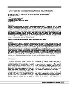
ˆ IQ degrades drastically as ω Figure 1 shows how the performance of K ˆ 0 moves away from the true value of ω0 , which happens in challenging environments when few data points are available. Our estimation technique, however, does not depend Estimating K with imperfect omega 2 IQ SDF
K Estimate
1.5
1
0.5
0 0.7
0.72
0.74 0.76 ω estimate
0.78
0.8
0
Fig. 1.
ˆ as ω K ˆ 0 varies (ω0 = 0.7447) via Monte Carlo simulation (80% of spectrum being used, Ω = 6, K = 2, N=1,000, and 100 simulations).
as strongly on ω ˆ 0 , correctly estimating K over the full range of ω0 searched. ˆ SDF with the other estimators mentioned by plotting their mean squared error Figure 2 compares the performance of K (MSE) vs. K. We see that the SDF technique dominates both IQ and MOME in the challenging environment of few available sample points and low SNR when enough spectrum is used in estimating σ 2 (80% or 90%). When the SNR is higher, the SDF technique performs comparably to the other estimators presented when 80% of the spectrum is used. Note that the low ˆ SDF increases as the percentage of spectrum used increases from 70% to 90% but at the expense of SNR performance of K decreasing its high SNR performance. We also note that the three techniques are comparable in computational complexity. When run in a MATLABTM Monte Carlo simulation of 10,000 trials containing 1,000 data points each, MOME completed in 58 seconds, IQ in 70 seconds, and SDF in 77 seconds. IV. B ROADBAND E XTENSION We now consider an alternate model of the received signal. Suppose that instead of the single tone model of Equation 1, the data is modeled as: X[n] = sej(f [n]+φ0 ) + Z[n]
(10)
which is to say that the signal can have some time-varying frequency content. As long as the signal is bandlimited and the sampling rate is high enough, then some amount of the estimated SDF will represent frequencies with noise dominated content (assuming that the spectrum has free bandwidth somewhere in the range of sampled frequencies) and can be used for ˆ SDF . In practice, the actual percentage of bandwidth chosen for use will depend on several factors including SNR, sampling K bandwidth, signal bandwidth, and any tapering that may be applied to improve spectral estimates. Table II shows the results of the estimation techniques applied to these bandlimited signals. We see that the IQ estimation breaks down for this data no matter which technique for estimating ω0 is used. MOME fails in this situation as well because we are dealing with low ˆ SDF performs well at 80% of the spectrum used but appears to degrade with more spectrum used. This is likely to SNRs. K
IEEE COMMUNICATIONS LETTERS, VOL. ?, NO. ?, JANUARY 200?
ˆ K
COMPARISON WHEN THE DATA IS BANDLIMITED AS IN
4
TABLE II E QUATION 10 (1,000 SIMULATIONS /
Estimate ˆ M LE Ω ˆ M OM E K ˆ IQ , FG K ˆ IQ , ZP K ˆ IQ , NR K ˆ SDF , 80% K ˆ SDF , 85% K ˆ SDF , 90% K
Mean 2.1021 0.1426 0.0077 0.0084 0.0086 0.0564 0.0218 0.0176
TECHNIQUE , Ω
= 2.1, K = 0.05,
AND
N = 1, 000).
Std Dev 0.0669 0.1715 0.0013 0.0014 0.0017 0.0345 0.0308 0.0240
ˆ SDF . due to non-empty spectrum being used to create a larger estimate of σ ˆ 2 and thus lower estimate of K MSE vs. K
3
10
MOME IQ SDF, 70% SDF, 80% SDF, 90%
2
10
1
MSE
10
0
10
−1
10
−2
10
−3
10
Fig. 2.
−2
10
−1
10
0
K (or SNR)
10
1
10
MSE of K estimators via Monte Carlo simulation (ω0 = 0.7447, ω ˆ 0 = 0.7257, N = 10, and 3,000 simulations)
V. C ONCLUSION We have presented a new technique for estimating the Ricean K parameter, utilizing the phase information of the complex Gaussian data from which it arises. The technique performs comparably to or better than (depending on how much of the spectrum is used) IQ estimation but allows for much imprecision in estimating ω 0 . It is also easily applied to signals with time-varying frequency content of either a deterministic or stochastic nature. More detailed information can be found in [8] including analysis of estimator performance over varying sample sizes and varying percentages of spectrum used in the SDF technique. R EFERENCES [1] A. Abdi, C. Tepedelenlioglu, M. Kaveh, and G. Giannakis, “On the estimation of the K parameter for the Rice fading distribution,” IEEE Comm. Letters, vol. 5, pp. 92–94, Mar. 2001. [2] Y. Chen and N. C. Beaulieu, “Estimation of Ricean and Nakagami distribution parameters using noisy samples,” in IEEE Trans. on Comm., 2004, pp. 562–566. [3] K. K. Talukdar and W. D. Lawing, “Estimation of the parameters of the Rice distribution,” J. Acoust. Soc. Amer., vol. 89, pp. 1193–1197, 1991. [4] C. Tepedelenlioglu, A. Abdi, and G. B. Giannakis, “The Ricean K factor: Estimation and performance analysis,” IEEE Trans. on Wireless Comm., vol. 2, pp. 799–810, Jul. 2003.
IEEE COMMUNICATIONS LETTERS, VOL. ?, NO. ?, JANUARY 200?
[5] J. G. Proakis, Digital Communications.
5
Boston: McGraw-Hill, 2001.
[6] G. R. Shorack, Statistics with Probability.
New York, NY: John Wiley & Sons, Inc., 2008.
[7] D. B. Percival and A. T. Walden, Spectral Analysis for Physical Applications.
Cambridge: Cambridge University Press, 1993.
[8] A. N. Morabito, “Ricean parameter estimation using phase information in low SNR environments,” Master’s thesis, Univ. of Washington, 2007.