estimate of an underlying scalar signal z(t) via a linear com- bination of the ..... the output 2(t) at the bot tom. ... Prentice-Hall, Inc., Englewood Cliffs, NJ, 1985.
RLS ADAPTIVE FILTERING WITHOUT A DESIRED SIGNAL: QR ALGORITHMS AND ARCHITECTURES Paul S. Lewis Los Alamos National Laboratory* Mechanical and Electronic Engineering Instrumentation Group MEE-3, MS 5580 Los Alamos, NM, 87545, U.S.A. filter computes an exact solution at each step based on the estimated correlations. An RLS adaptive filter can be implemented by either the traditional Kalman RLS algorithm [I], in which the inverse of the estimated autocorrelation matrix is recursively computed, or by the RLS/QR algorithm, in which the QR decomposition of the data matrix is recursively computed [1,2].Of the two approaches, the QR formulation has superior numerical and structural properties. In many applications, a desired signal does not exist, but partial a priori information, in the form of the signal-to-data cross-correlation vector, is available. In these situations, a "mixed" adaptive filter may be employed in which only the autocorrelation matrix C,,(t) is estimated. This estimate is obtained from the sample matrix of the past data. One example of this mixed situation is beamforming, in which the cross-correlation vector corresponds to the steering vector. The least mean square (LMS) family of algorithms (31, based on steepest descent, contains the P-vector algorithm that addresses this case 141. To overcome the disadvantages of a steepest descent approach, recursive sample matrix inversion (SMI) algorithms have been proposed (5,6]. They are based on a recursive update of the inverse of the sample matrix and have a structure similar t o the Kalman RLS algorithm. Like the Kalman RLS algorithm, they suffer from both numerical and structural problems. The paper demonstrates how the mixed filter can be formulated as a least squares problem and stable QR decomposition-based techniques used in its solution. This formulation leads to algorithms with the performance, numerical, and structural advantages of the RLS/QR algorithm, but without the requirement of a desired signal. These algorithms are easily implemented by triangular or linear systolic arrays.
Abstract Most adaptive filters require a desired signal for operation. However, in many applications the a priori knowledge consists of the signal-to-data cross-correlation vector rather than a desired signal. Recursive sample matrix inversion (SMI) algorithms exist for this "mixed" case. These SMI algorithms, which are based on the inversion of a data correlation matrix, have both numerical and structural shortcomings. This paper demonstrates how to formulate the recursive solution to the mixed case as a least squares problem. This formulation leads to algorithms based on recursive QR decomposition implemented by either Givens or fast Givens rotations. Compared to the recursive SMI approach, these QR-based algorithms are more efficient, have better numerical properties, and exhibit greater structural regularity. Because of their structural regularity, the algorithms are easily implemented by either a triangular or linear systolic array.
1
Introduction
Recursive least squares (RLS) adaptive filters compute an estimate of an underlying scalar signal z ( t )via a linear combination of the input data ? ( t ) = w'(t)y(t),where y ( t ) is the n-dimensional input vector, w(t)the n-dimensional weight vector, and the prime denotes transpose. The optimal filter can be expressed in terms of the autocorrelation matrix C,,(t) E E { y ( t ) $ ( t ) } and signal-to-data cross-correlation vector c',,(t)= E { z(t)y'(t)} 111.
q t ) = C(,,(t)C;;(t)y(t) .
(1)
If C,,(t) and G',,(t) are know a priori, then (1) may be implemented directly. However, in many cases these correlations are unknown. For quasi-stationary signal and data, an adaptive filter can be used to provide an approximation of this optimal filter based on past inputs. The autocorrelation matrix can be estimated from the data alone, but estimation of the signal-to-data cross-correlation vector requires a desired signal. Given a desired signal, an RLS adaptive
2
Given the signal-to-data cross-correlation vector C'%,(t), the mixed filter can be defined as
? ( t ) = c',,(t)&;,'(t)y(t)
'Los Alamos National Laboratory is operated by the University of California for the U.S. Department of Energy under contract W-7405-
ENG-36
49 22ACSSC-12/8810049 $1.00
01988 MAPLE PRESS
Algorithms
,
(2)
where the sample matrix & ( t ) is an estimate of the autocorrelation matrix C,,(t) based on the data available at
2.2
time t. A common causal and recursive estimate of C,,(t) is = xze,,(t- 1) + (1 - X")y(t)y'(t) 9 (3)
QR Recursions
Tlie equivalent least squares problem in (8) can be solved by a recursive QR algorithm similar to those used in RLS filters with a desired signal. The QR decomposition of the data matrix is
e,&)
where X2 is an exponential "forgetting" factor ranging between zero and one that weighs recent data more heavily. The recursive SMI approach applies the matrix inversion lemmqto the &(t) update to yield a direct recursive update of C;J(t) [5,6]. This approach requires 3rn2 4rn operations per time step (71. Here an operation is defined as a multiplication or division and, optionally, an addition or subtraction. This type of algorithm suffers from two major disadvantages. The first disadvantage is numerical. Recuris poorly conditioned because it sive estimation of involves inversion of a data correlation matrix. The condition number of a data correlation matrix is the square of the condition number of the corresponding data matrix, hence twice the dynamic range is required in the numerical computations (81. The second disadvantage is structural. The form of the recursive update ,of C;;(t) severely limits the parallelism and pipelining that can be effectively applied in implementation (71.
-
-
(9)
+
where Q', is a t x t orthogonal matrix and Rt is an rn x rn upper triangular matrix. This decomposition can be used to solve for h, by first multiplying both sides of Y& = 21. by Qt?
e;l(t)
2.1
and then solving the resulting rn x m triangular system = R;l& [8].Here e is an rn-dimensional vector, and indicates "don't care." To avoid solving a growing system at each time step, a recursive QR formulation may be used that computes the new triangular factor by rotating the added row )y'(t) into the previous triangular factor XR:-l. The form of the recursive QR update is IS]
h,
Least Squares Formulation
To avoid both the numerical and striictural difficulties associated with the recursive SMI approach, the mixed filter can be formulated as a least squares problem. To begin this formulation, the sample matrix C , , ( t ) is expressed as a weighted data correlation matrix-in Y'Y form. Given data g( 1) . . .y ( t ) ,define the m x t weighted data matrix as Yft= [ P y ( t ) X'y(t - 1)
...
X"'y(l)]
.
=
Q:
The middle rows of zeros are not affected by the rotation Q, and can be ignored. The update can therefore be expressed more compactly as
(4)
This definition permits the sample matrix to be expressed as = (1 - A Z ) Y',Yt (5)
e&)
.
where Q t is a "compressed" version of Q t .
By defining a "pinning" vector E' (1 0 01, ~ ( tcan ) be Substituting . these definitions into expressed as y ( t ) = Y t t ~ (2) allows the mixed filter to be cast in the normal equation form ? ( t ) = (1- Xz))-lC'z,(t) (Y'tYt)-ly't~. (6) 9 . .
2.3
QR Update-Givens
Rotations
The most straightforward way of implementing the QR updale of (12) is through Givens rotations (81. These are orDefining the m-dimensional vector & = (Y'tYt)-'Y't~ thogonal transforms that zero one element a t a time. Updated Rt matrices are computed by zeroing the elements leads to of the added row from left to right via a series of Givens ,qt)- C'Z&)b (7) 1-xz . rotations. In (12) this series corresponds to The unknown vector b can be found by solving Y',Ytht = Q t = ($4.. . , Ylta, which is equivalent to finding a least squares solution (13) to the overdetermined system where zeros the ith element in the first row by rotating it with the (i 1)st row. An individual rotation is of the Yth, = . (8) form e -8 The end result of this least squares formulation is a method I of calculating b,and from it ? ( t ) , directly from the data (14) s C matrix Yt without forming and inverting the sample matrix
Qy'Qy'
Qii)
+
I
Y'tY,.
50
and affects only the first and (i + 1)st rows. The effect on these two rows is
[ ," -PI [ ... [ ... 0
=
0
0
0
Y(i)
Y(i+l)
**.
0
0
'(i)
r(i+l)
.' .
I . .
0 0
0 ?(I)
Rt
DtRt
,
and
rDt,
.
According to (12), the recursive update becomes
i(j+l) ?(I+')
=
. ..
To orthogonally zero Y ( ~ ) the , rotation factors are defined by
Computation of the rotation factors can be accomplished with four operations and a square root [SI. Application of the rotation requires four operations per column. Denoting the series of Givens rotations by %, the resulting algorithm can be expressed as
Recall from (13) that Qt is composed of a series of Givens rotations. In a similar manner, St is composed of a series of fast Givens rotations
s t = p ) .st* .s:w * . (') R;'e 2) ? ( t ) = (1 - A*)-'Cfzu(t)
(22)
Each individual fast Givens rotation can be related to the corresponding orthogonal Givens rotation by
,
where the Rt recursion is initialized by Ro = 0. The Givens update of step 1requires 2rn2+6rn operations and m square roots.
2.4
QR Update-Fast
for a' = 1 to rn, where diol = 1, dt = dim', DP1= and Dt = Df"'.
Givens Rotations
Although orthogonal Givens rotations provide a numt.rically stable way of coniputing the recursive Q R update, they have two drawbacks. The first is the square-root computation needed to compute the rotation factors. The second is the four operations per column needed to implement the rotation. Both of these drawbacks can be eliminated by the use of square-root-free or fast Givens rotations [2,8,9]. A fast Givens rotation approach to computing the QR decomposition modifies the form of (9) to the form
A-lDt-1,
There are numerous forms for fast Givens rotations that satisfy (23) and require only two operations and no square roots. The most commonly used forms are IS]
An algorithm that implements fast Givens rotations of these It is easily modified to two forms may be found in Ref. .]!I a recursive algorithm that, given Rt-1, D;-*, and ~ ( t com), putes R, and D: and applies the rotations to E to compute &. Note that it is D:, the square of the diagonal weight matrix, that is actually needed. Dt is never explicitly computed. Six operations are necessary to compute the rotation factors and two operations per column are then required to apply them. The only drawback of the fast Givens approach is that the D: matrices must be monitored for overflow [SI. By denoting the series of fast Givens rotations by F%' and observing that R;'% = RL'&, the resulting algorithm can be expressed as
?here Dt and Dt are diagonal matrices and the columns of DY'S;' are orthogonal, but not orthonormal. This decomposition is related to the original by
Use of St rather than Q t to compute the QR decomposition permits the form of the individual "rotations" to be simplified. The square-root computation can be eliminated and the number of operations needed per column can be reduced from four to two. This approach can be applied to recursive QR updates by partitioning the diagonal matrices and working only with the relevant nonzero rows of the decomposition as outlined in (12). Both the triangular and diagonal matrices must be recursively computed. To begin, define
51
Here the Rt recursions are initialized by R0 = 0. The fast ~i~~~~ update of step 1 requires only m2 + 7m operations per time step.
2.5
Solving the Triangular System
In either the Givens or fast Givens approach, the form of the second step of the algorithm is the same. There are two choices in implementing this step. These choices are computation of R;'% by back substitution, or computation of R';lC&(t) by forward elimination. On a general-purpose computer, both approaches are equivalent. However, the data Row of the forward elimination computation matches the data Row of the QR update, whereas the data flow of the back substitution is the reverse of the data flow of the QR update [7,10]. This makes the forward elimination approach the candidate of choice for array processor implementation. Note that the forward elimination approach used here is viable because the output s ( t ) is a scalar and hence the signal-to-data cross-correlation is a vector. In the general case of n output channels, the signal-to-data crosscorrelation is an n x m matrix and the forward elimination approach becomes much less computationally efficient than.the back substitution approach 171. Therefore, in the multiple output channel case it is necessary to use the back substitution approach and the resulting array architecture implementations are much less regular than those presented in the next section (7,101. Using forward elimination, the second step can be rewritten as 2a) Solve R't$ = ( 1 - A)-'Lv(t) 26) 2 ( t ) = q'te .
for gt
and
+
The forward elimination of step 2a requires (m2 3m)/2 operations [SI and the vector inner product of step 2b requires m operations. The total computation requirements per time step for each of the QR-based approaches and the recursive SMI (Y'Y) approach are: Algorithm Operations ,/QR-Givens 2.5m2 8.5m m QR-Fast Givens 1.5mZ 9.5m 0 Recursive SMI 3m2+4m o
+ +
Compared to the recursive SMI approach, the QR-based mixed filter algorithms presented in this paper offer not only improved numerical performance, but also increased efficiency.
2.6
have shown that, given adequate precision, the QR- based and Y'Y-based algorithms produce the same results. '"his finding demonstrates that, mathematically, the QR-ba yed algorithms provide a true RLS solution and possess all of the associated algorithmic advantages. However, in general, the QR-based algorithms were able to correctly operate with only one half of the precision required by the Y'Y-based algorithms. This result demonstrates that the QR-based approach does provide significant numerical advantages.
3
Architectures
Array architectures for implementing recursive QR updates, forward elimination, and vector-vector inner product are well known [ 1 , 2 , 7 ] . Recursive QR updates, using either Givens or fast Givens rotations, can be implemented by the triangular array structure shown in Fig. 1. The additional row $ ( t ) is fed in from the top and successively rotated with each row of the triangular factor Rt-1 stored in the array to produce the new triangular factor Rt. The rotation factors are computed in the diagonal elements and then propagated across rows. An additional column is included to explicitly apply the rotations to the pinning vector E to produce 3 . (An alternate approach is to map this computation onto the diagonal elements and propagate the result across the array.) The forward elimination computation can also map directly onto a triangular array structure with a data Row pattern identical to that of the QR update [7\. The elements of the vector c(,,(t) are fed in from the top and successively eliminated from the R't equations to produce the solution vector st at the right. Finally, the inner product s't% is computed in the last column to produce the output 2 ( t ) at the bot tom. Figure 1 depicts the triangular array structure as a signal flow graph (SFG) in which communication along the arcs is delay-free. A systolic implementation with unit delays on each arc may be obtained by retiming [ 1 1 , 1 2 ] . This retiming amounts to adding delays to each arc and appropriately skewing the inputs. No pipeline interleave is required. For m input channels, the result is an array with (m2 3m)/2 nodes, a latency of 2m, a computation time of 3m, and a throughput of 1 (71. Using multiprojection mapping techniques [11,12], a linear array can be derived by projection of the SFG nodes in a horizontal direction (71. For the linear array, the latency and computation times remain unchanged. However, the throughput decreases to l / ( r n + 1 ) .
+
4
Simulations
The QR-baqed mixed filter algorithms present,ed in Illis paper are new. A number of simulations have been run to verify their functionality and compare them to Y'Y-based approaches, such as the recursive SMI algorithm. Details of the simulations may be found in Ref. 17). The simulations
Summary
This paper has presented a pair of adaptive QR decomposition-based algorithms for the mixed adaptive filter in which no desired signal is available, but the signalto-data cross-correlation vector is known. These algorithms match the performance of recursive SMI approaches, but
52
provide increased efficiency, superior numerical properties, and more structural regularity. The algorithms were derived by first formulating the recursive mixed filter as a least squares problem and then applying orthogonal QR-based techniques in its solution. Both Givens and fast Givens rOtations were used in implementing the recursive QR decomposition. The Givens approach requires 2.5m2 8.5m operations and m square roots per time step, whereas the fast Givens approach requires only 1.5m2 9.5m operations and no square roots. The algorithms consist of regularly structured computations and data flow and can be implemented by either a triangular or a linear systolic array.
LO] P. S. Lewis. Algorithms and architectures for multichannel enhancement of magnetoencephalographic sig-
nals. In Proc. 21st Asilomar Conf. on Signals, Systems, and Computers, pages 741-745, IEEE, Pacific Grove. CA, November 1987.
+
111 S. Y. Kung, S. N. Jean, S. C. Lo, and P. S. Lewis. Design methodologies for systolic arrays: mapping al-
+
gorithms t o architecture. In Chen, editor, Signal Processing Handbook, chapter 6, pages 145-191, Marcel Dekker, Inc., New York, NY, 1988. (121 S. Y. Kung. VLSI Array Processors. P rent ice- Hall, Inc., Englewood Cliffs, NJ, 1988.
References [l] S. Haykin. Adaptive Filter Theory. Prentice-Hall, Englewood Cliffs, NJ, 1986. [2] J. G. McWhirter. Recursive least-squares minimization
using a systolic array, In Real Time Signal Processing VI, page 105, SPIE, 1983. Y l c1
[3]B. Widrow and S. D. Steams. Adaptive Signal Processing. Prentice-Hall, Inc., Englewood Cliffs, NJ, 1985.
YZ
c2
Y3
c3
Y4 c4
1 0
[4]L. J. Griffiths. A simple adaptive algorithm for real-time processing in antenna arrays. Proc. IEEE, 57:1696-1704,March 1969. [5]R. A. Monzingo and T. W. Miller. Introduction to Adaptive Arrays. John Wiley & Sons, New York, NY, 1980. [6]R. T. Compton. Adaptive Antennas. Prentice Hall, Englewood Cliffs, NJ, 1988.
(71 P. S. Lewis. Algorithms and Architectures for Adaptive Least Squares Signal Processing, with Applications in Magnetoencephalography. PhD thesis, University of Southern California, Dept. Electrical EngineeringSystems, Los Angeles, CA, August 1988. Los Alamos National Laboratory report LA-11409-T,October 1988. 181 G. H. Golub and C. F. Van Loan. Matriz Computations. The Johns Hopkins University Press, Baltimore, MD, 1983.
Figure 1: Triangular signal pow graph array for the QR-based mized filter algorithms.
19) J. H. Wilkinson. Some recent advances in numerical lin-
ear algebra. In D. Jacobs, editor, The State of the Art in Numerical Analysis, pages 3-54, Academic Press, New York, NY, 1977.
53