In this experiment, a mobile unit was moved from 5 to 28 meters away from the access point ... 250 packets of 1000 bytes per second (2 Mbps). In level 2, 125 ...
Adaptive Streaming Based on IEEE 802.11 Signal Quality Arlindo Flávio da Conceição1 ∗, Fabio Kon1 1
Distributed Systems Research Group – Department of Computer Science Institute of Mathematics and Statistics – University of São Paulo (DCC - IME/USP) http://gsd.ime.usp.br {arlindo,kon}@ime.usp.br
Abstract. In order to transmit over wireless networks, streaming applications must provide adaptive strategies for problems such as mobility and handoffs. This work presents an algorithm for adaptive streaming over IEEE 802.11 networks that adapts the transmission in function of the perceived signal quality and, by doing this, improves the transmission efficiency and the network utilization.
1. Introduction In the last years the usage of IEEE 802.11 networks (also called Wi-Fi) has strongly increased. Despite this, the design of application layer adaptive techniques for these networks have not received the appropriate attention. In fact, we have seen a small number of products, and even articles, that report the application layer strategies in details [Vandalore et al., 2001]. This work presents an algorithm for adaptive streaming over IEEE 802.11 networks. To do this, we first show how to get signal quality information and how this information is related to the actual network capacity. After this, we present our algorithm and the results achieved. Finally, we present our conclusions.
2. How to get information about wireless connection In Windows systems, the information about wireless cards can be easily accessed by using the ndisprot protocol driver (see http://ramp.ucsd.edu/pawn/wrapi). In Linux, the simplest way to do this is using the pseudo-file /proc/net/wireless1 . In this work we used Linux and, for our purposes, the most relevant information in the pseudo-file /proc/net/wireless are: • link: quality of the link (how good the received signal is); • level: received signal strength (how strong the received signal is); • noise: background noise strength when no packet is transmitted. For the sake of simplicity from now on, we refer to these signal quality parameters as quality, signal and noise. In addition, we will extensively use SNR (signal noise Ratio) in the second part of this text. ∗
Suported by CNPq, grant 141415/2002-9. It is important to notice that the content of the pseudo-file /proc/net/wireless may vary a lot in function of the drivers used. For further information see [WildPackets, 2002] and http://www.hpl. hp.com/personal/Jean_Tourrilhes/Linux/Wireless.html 1
3. Signal quality and network capacity Figure 1 shows the variation of signal quality and network capacity in presence of mobility. In this experiment, a mobile unit was moved from 5 to 28 meters away from the access point, and then it was brought back. Figure 1(a) shows the variation of signal and its impact in the transmission rate, the results confirm that: • Signal varies in function of the distance from the access point; • Noise presents only very small variations; • The reception capacity is strongly related to signal.
220
4
3
3.5
200
3
190
2.5
2
180
1.5
170
1
160 0
20
40
60
80 Time (s)
100
120
140
160
(a) Signal and transmission rate variation
2.5
Reception rate (Mbps)
210
Transmission rate (Mbps)
Signal and noise strength
Reception rate Signal Noise
2
1.5
1
0.5
0 1.05
1.1
1.15
1.2 1.25 Signal Noise Rate (SNR)
1.3
1.35
1.4
(b) SNR and transmission rate correlation
Figure 1: Signal and transmission rates in presence of mobility
As expected, the data stream, initially of 2 Mbps, suffers expressive losses when the value of signal is low. It is important to notice that the losses occur mainly when signal reaches a certain lower threshold. Moreover, when signal gets close to Noise, the network operates in a more unstable way (with losses and peaks of transmission). In fact, as expected [Schiller, 2000], the network becomes inoperative when signal reaches smaller levels than noise. Note that mobility is not the only reason for transmission interference, there might be also interfering factors such as radio devices [Golmie et al., 2003], network traffic [Heusse et al., 2003, da Conceição and Kon, 2003], and appliances like microwave ovens. Figure 1(b) plots the relation between SNR and the transmission rates achieved. It shows a cloud of points that can be divided into three parts. First, the right-hand side where SNR is high and the transmission rate is stable around 2 Mbps. Second, the middle area, where transmission is unstable but still reaches 2 Mbps in average. Finally, a third area, at the left-hand side, where SNR is low and the rate of 2 Mbps is rarely reached. Based on these areas, we can define two thresholds, α and β, where α is the smallest SNR value such that the transmission is considered good and, similarly, β is the smallest SNR value such that the transmission is acceptable. For example, in Figure 1(b), α and β could be 1.15 and 1.1, respectively.
4. Adaptive streaming based on α and β thresholds In order to optimize network utilization, considering a client/server streaming application, our algorithm adapts the streaming in function of signal quality information. It uses SNR, α and β, as follow:
• Level 0: If SNR ≥ α, then the server transmits normally; • Level 1: If α > SNR ≥ β, then the server acts in a conservative way, for example reducing the packet size; • Level 2: If β > SNR ≥ 1, then the server reduces the transmission rate. • Level 3: If SNR < 1, then the transmission is interrupted until SNR > 1. The adaptive strategy is organized in levels such that clients can automatically find the α and β thresholds in function of its reception quality and application requirements. The algorithm could also keep the thresholds dynamically updated; our experiments, however, showed similar performance between static and dynamic usage of α and β. After found, we believe that is not necessary to frequently update the thresholds. But they must be recalculated in case of network configuration changes as, for example, when handoffs occur. 4.1. Experimental results Figure 2 shows one instance of our experiments that compares the adaptive and the nonadaptive streamings. This experiment uses α = 1.13 and β = 1.09. In adaptive level 0, the server transmits 125 packets of 2000 bytes per second (achieving 2 Mbps). In level 1, 250 packets of 1000 bytes per second (2 Mbps). In level 2, 125 packets of 1000 bytes per second (the transmission rate is reduced to 1 Mbps). And in level 3, the server interrupts the transmission for three seconds. 3.5
4 Non-adaptive algorithm transmission rate Adaptive algorithm transmission rate Adaptive level
3 3
2
2
1.5
1
Adaptive level
Transmission rate (Mbps)
2.5
1 0 0.5
0 20
30
40
50 Time (s)
60
70
80
Figure 2: Non-adaptive and adaptive algorithms executions
In Figure 2, we can see that, initially (from 20 to 30s approximately), both algorithms achieve 2 Mbps. In addition, from 30 to 55s, both algorithms do not achieve the rate of 2 Mbps when the mobile unit is far from the access point. But there is an expressive difference in how the algorithms recover the transmission (from 55 to 75s). In general, the non-adaptive algorithm takes longer to recover the normal transmission after a movement period. In our experiments, which were exhaustively repeated, the adaptive algorithm consistently recovered the desired transmission rates much faster than the non-adaptive. This was the key reason for the better performance of the adaptive algorithm. Table 1 summarizes the results. It shows that the adaptive client received more data than the non-adaptive, even the server sending more data to the non-adaptive algorithm; in other words, it was much more efficient2 . In consequence, the adaptive algorithm 2
Efficiency is defined as the amount of received data divided by transmitted data and must be as close as possible to 1.
Algorithm Non-adaptive Adaptive
Transmitted Received 1848 Mbits 1390 Mbits 1659 Mbits 1604 Mbits
Average rate 1.505 Mbps 1.736 Mbps
Efficiency 0.75 0.96
Table 1: Comparison of data transmitted and effectively received
achieved transmission rates 15% higher than the non-adaptive one, 1.7 Mbps against 1.5 Mbps. Moreover, scenarios where this difference is even more expressive could be easily showed by, for example, setting experiments with longer periods of disconnection.
5. Conclusion and future work This work analyzed the design of adaptive applications based on signal quality of IEEE 802.11 networks. It showed the feasibility of such applications and described an implemented algorithm for improved network usage. By considering the network conditions, our adaptive algorithm reduced the waste of network capacity and, consequently, increased the effective throughput. The adaptive algorithm transmitted 15% more data than the non-adaptive algorithm and it was more efficient; what is specially important for IEEE 802.11 networks because of the automatic re-transmission mechanism used in the MAC layer [Gast, 2002]. Despite these results, it is important to remember that α and β must be chosen in function of interfaces and access points used; in the programmers’ dialect, the thresholds cannot be hard-coded. With this short paper, we hope to help application developers interested in distributing content over wireless networks. In practice, it is still pretty hard to conduct reproducible experiments in IEEE 802.11 networks, but it is possible, and relatively easy, to implement strategies that actually improve communication over these networks. In our ongoing work, we are refining the adaptive strategies presented here to apply them to MPEG-4 video streaming.
References da Conceição, A. F. and Kon, F. (2003). Adaptação de fluxos contínuos UDP sobre redes IEEE 802.11b. In Workshop de comunicação sem fio e computação móvel (WCSF), pages 91–101, São Lourenço-MG, Brasil. Gast, M. S. (2002). 802.11 Wireless Networks. The definitive Guide. O’Reilly. Golmie, N., Chevrollier, N., and Rebala, O. (December 2003). Bluetooth and WLAN coexistence: Challenges and solutions. IEEE Wireless Communications Magazine, 10(6):22– 29. Heusse, M., Rousseau, F., Berger-Sabbatel, G., and Duda, A. (2003). Performance anomaly of 802.11b. In IEEE Infocom, San Francisco, CA, USA. Schiller, J. (2000). Mobile Communications. Addison Wesley. Vandalore, B., chi Feng, W., and Raj Jain, S. F. (2001). A survey of application layer techniques for adaptive streaming of multimedia. Real-Time Imaging, 7(3):221–235. WildPackets (2002). Converting signal strength percentage to dBm values. Available in http://www.wildpackets.com/elements/whitepapers/ Converting_Signal_Strength.pdf. Last visit in December 2004.