RNA Secondary Structure Design under Simple and Complex

RNA Secondary Structure Design under Simple and Complex Constraints

Dissertation zur Erlangung des akademischen Grades doctor rerum naturalium (Dr. rer. nat.)

vorgelegt dem Rat der Fakultät f¨ ur Angewandte Wissenschaften der Albert-Ludwigs-Universität Freiburg

von Diplom-Wirtschaftsmathematikerin Anke Busch

Dekan: Prof. Dr. Bernhard Nebel Gutachter: Prof. Dr. Rolf Backofen Prof. Dr. Peter F. Stadler Datum der Promotion: 03. Juni 2008

RNA Secondary Structure Design under Simple and Complex Constraints Anke Busch January 2008

ii

Abstract The structure of RNA molecules is often crucial for their function. Therefore, designing RNA sequences that fold into a given structure with special features is of interest for biologists in several fields. In this thesis, we introduce two approaches dealing with RNA sequence design. First, we develop a fast and successful new approach to the inverse RNA folding problem, called INFO-RNA, incorporating constraints on the sequence, while afterwards, our interests focus on a more complex design of RNA sequences taking into account the translated amino acid sequences. We develop an algorithm, called SECISDesign, that solves this complex task successfully. In the first part of this thesis, we focus on the search for an RNA sequence S = S1 ...Sn that folds into a given secondary structure T and fulfills given constraints C = C1 ...Cn on the primary sequence. Our new approach INFO-RNA consists of two parts; a dynamic programming method for good initial sequences and a following improved stochastic local search that uses an effective neighbor selection method. During the initialization, we design a sequence that among all sequences adopts the given structure with the lowest possible energy. There is no other sequence that has lower energy when folding into this structure. Nevertheless, the sequence is not guaranteed to fold into T since it can have even less energy when folding into another structure. Therefore, the resulting sequence is processed further using a stochastic local search. For the selection of neighbors during this search, we use a kind of look-ahead of one selection step applying an additional energy-based criterion. Afterwards, the pre-ordered neighbors are tested using the actual optimization criterion of minimizing the structure distance between the target structure and the structure of the considered neighbor with minimal free energy or maximizing the probability of folding into T . We compare INFO-RNA to the two existing tools RNAinverse and RNA-SSD using artificial as well as biological test sets. Running INFO-RNA, we perform better than RNAinverse and in most cases, we obtain better results than RNA-SSD, the probably best inverse RNA folding tool on the market.

iv

Abstract The second part of this thesis concentrates on a more complex design of RNA sequences. Here, not only the secondary structure of the RNA sequence is taken into account but also the amino acid sequence, which is encoded by the designed RNA. Thus, this part of the thesis can be applied to the design of coding parts of mRNA sequences. The most prominent example is the application to selenoproteins. These are proteins containing the 21st amino acid selenocysteine, which is encoded by the STOP-codon UGA. For its insertion it requires a specific mRNA sequence downstream the UGA-codon that forms a hairpin-like structure (called selenocysteine insertion sequence (SECIS)) and codes for the amino acids following the selenocysteine in the protein. Selenoproteins have gained much interest recently since they are important for human health. In contrast, very little is known about them. One reason for this is that one is not able to produce enough amount of selenoproteins by using recombinant expression in a system like E.coli straightforwardly since the selenocysteine insertion mechanisms are different between E.coli and eukaryotes. Thus, one has to redesign the human/mammalian selenoprotein for the expression in E.coli. In this thesis, we introduce an polynomial-time algorithm, called SECISDesign, for solving the computational problem involved in this design and present results for known selenoproteins. In the third part of this thesis, we introduce two web services, which make it possible to use our two algorithms online. They introduce the programs INFO-RNA and SECISDesign to a wide community of scientists and allow them to design RNA sequences in an automatic manner. They allow to use INFO-RNA and SECISDesign without compiling their source codes and even without having an executable version of them on the local computer. To conclude, both, INFO-RNA and SECISDesign, are fast and successful tools for the design of RNA sequences dealing with simple and complex constraints, respectively. They outperform existing tools and methods for most structures.

Zusammenfassung Die Struktur von RNA Molek¨ ulen ist oft entscheidend f¨ ur ihre Funktion. Deshalb ist das Design von RNA Sequenzen, die in eine gegebene Struktur falten, von großem Interesse in der derzeitigen Forschung. In dieser Arbeit stellen wir zwei neue Ansätze vor, die sich mit dem Design von RNA Sequenzen beschäftigen. Im ersten Teil entwickeln wir einen schnellen und erfolgreichen Ansatz (INFO-RNA) zur Lösung des inversen RNA Faltungsproblems. Im zweiten Teil geht es um ein weitaus komplexeres Designproblem. Hier stellen wir den Ansatz SECISDesign vor, der sich mit dem Design von kodierenden RNA Sequenzen beschäftigt und deshalb zusätzlich die von der designten mRNA kodierte Aminosäuresequenz ber¨ ucksichtigt. Im ersten Teil dieser Dissertation geht es um das inverse RNA Faltungsproblem mit einigen Einschränkungen der möglichen Sequenz. Mit anderen Worten, es geht um die Suche nach einer RNA Sequenz S = S1 ...Sn , die sich in eine gegebene Sekundärstruktur T faltet und zusätzlich gegebene Bedingungen C = C1 ...Cn an die RNA Sequenz erf¨ ullt. Unser neuer Ansatz, INFO-RNA, besteht aus zwei Teilen: einem dynamischen Programmierverfahren zur Erzeugung einer initialen Sequenz und einer anschließenden erweiterten stochastischen lokalen Suche, die eine neue effektive Methode zur Kandidatenauswahl benutzt. Durch die Initialisierung finden wir eine Sequenz, die die gegebene Struktur mit der geringsten möglichen freien Energie annimmt. Es gibt keine andere Sequenz, die eine geringere freie Energie hat, wenn sie in T faltet. Trotzdem kann nicht garantiert werden, dass sich unsere designte Sequenz S in die gew¨ unschte Struktur T faltet, da S selbst in eine andere Struktur mit geringerer freier Energie falten könnte. Deshalb wird die initial-gefundene Sequenz durch eine anschließende lokale Suche bez¨ uglich ihrer Faltungseigenschaft weiter verbessert. Während dieser Suche verwenden wir ein zusätzliches Energiekriterium, dass uns erlaubt, einen Schritt vorauszublicken. Nachdem alle Sequenzkandidaten durch dieses Kriterium in eine Reihenfolge (entsprechend ihrer G¨ ute) gebracht wurden, werden sie mit dem eigentlichen Suchkriterium gepr¨ uft. Hierbei wird versucht, die Distanz zwischen der Zielstruktur T und der Struktur mit minimaler freier Energie der designten Sequenz zu minimieren oder die Faltungswahrscheinlichkeit f¨ ur T zu maximieren.

vi

Zusammenfassung Wir vergleichen INFO-RNA mit den beiden existierenden Programmen zur inversen RNA Faltung, RNAinverse und RNA-SSD. Dazu verwenden wir sowohl k¨ unstlich generierte also auch biologisch real existierende Datensätze. Es zeigt sich, dass INFO-RNA schneller bessere Ergebnisse liefert als die beiden Vergleichsprogramme. Der zweite Teil der Dissertation beschäftigt sich mit einem komplexeren Design von RNA Sequenzen. Es wird nicht nur die gew¨ unschte Sekundärstruktur betrachtet sondern auch die Aminosäuresequenz, die durch die designte RNA Sequenz kodiert wird. Somit kann dieser Teil der Arbeit zum Design von kodierenden Teilen der mRNA benutzt werden. Das bekannteste Beispiel ist die Anwendung des Programms auf Selenoproteine. Diese sind Proteine, die die 21ste Aminosäure Selenocystein enthalten, die durch das sonstige Stopcodon UGA kodiert wird. Um Selenocystein einzubauen ist eine spezielle mRNA Sequenz strangabwärts des UGACodons notwendig, die eine haarnadel-ähnliche Struktur ausbildet. Sie wird ”selenocysteine insertion sequence” (SECIS) genannt und kodiert außerdem f¨ ur die Aminosäuren, die dem Selenocystein folgen. Während der vergangenen Jahre sind Selenoproteine immer mehr ins Interesse der Forschung ger¨ uckt. Trotzdem ist relativ wenig u ¨ ber sie bekannt. Das liegt daran, dass es nur schwer möglich ist, große Mengen von ihnen in einem rekombinanten Expressionssystem wie E.coli herzustellen, da der Einbau von Selenocystein in E.coli anders funktioniert als in Eukaryoten. Deshalb muss die RNA eukaryotischer Selenoproteine f¨ ur die Expression in E.coli umdesignt werden, so dass sie das SECIS-element an der f¨ ur E.coli notwendigen Position haben. In dieser Arbeit stellen wir den polynomiellen Algorithmus SECISDesign vor, der dieses Designproblem löst und präsentieren außerdem Ergebnisse f¨ ur bekannte Selenoproteine des Menschen und der Maus. Im dritten Teil dieser Arbeit stellen wir zwei Webserver vor, durch die es möglich ist, unsere Programme INFO-RNA und SECISDesign online zu benutzen und sie somit einer breiten Masse von Wissenschaftlern zugänglich zu machen. Abschließend bleibt zu sagen, dass INFO-RNA und SECISDesign zwei schnelle und erfolgreiche Programme zum Design von RNA Sequenzen sind, die besser und schneller arbeiten als andere existierende Verfahren.

Danksagung Mein erster Dank gilt meinem Doktorvater Rolf Backofen. Ihm danke ich f¨ ur die Betreuung dieser Arbeit, viele interessante Diskussionen, f¨ ur die gute und erfolgreiche Zusammenarbeit aus der einige gemeinsame Publikationen entstanden sind, sowie f¨ ur seinen Enthusiasmus und die Inspiration zu neuen Ideen. Bedanken möchte ich mich bei Peter Stadler f¨ ur das Interesse an meiner Arbeit und die Bereitschaft, diese Dissertation zu begutachten. Desweiteren möchte ich mich bei meinen Kollegen und ehemaligen Kollegen am Lehrstuhl f¨ ur Bioinformatik zunächst in Jena und später in Freiburg Michael Beckstette, Steffen Heyne, Michael Hiller, Martin Mann, Rainer Pudimat, Andreas Richter, Sven Siebert und Sebastian Will f¨ ur viele interessante und hilfreiche Diskussionen sowie f¨ ur all die gemeinsamen Unternehmungen bedanken. Außerdem gilt ¨ mein Dank Monika Degen-Hellmuth f¨ ur die Hilfe beim Uberwinden aller b¨ urokratischen H¨ urden. F¨ ur das Korrekturlesen dieser Arbeit bedanke ich mich bei Michael Hiller und Martin Mann. Besonders bedanken möchte ich mich bei meinem Zimmerkollegen Michael Hiller f¨ ur seine Unterst¨ utzung, viele hilfreiche Tipps, interessante Diskussionen und nicht zuletzt f¨ ur das Ertragen meiner ”kommunikativen” Phasen und die häufig etwas höhere Raumtemperatur. Außerdem bedanke ich mich bei meiner Mutter Monika f¨ ur ihre immerwährende Unterst¨ utzung, ihr allzeit offenes Ohr und ihre Liebe, ohne das alles diese Arbeit nicht möglich geworden wäre. Last but not least möchte ich mich bei meinem Freund Martin bedanken, der mich nun schon seit vielen Jahren liebevoll begleitet und unterst¨ utzt, mich auch in schwierigen Situationen wieder aufbaut und mir neuen Mut gibt.

viii

Danksagung

List of Own Publications [1] Sebastian Will, Anke Busch, and Rolf Backofen. Efficient sequence alignment with side-constraints by cluster tree elimination. Constraints Journal, 2008, to appear. [2] Anke Busch and Rolf Backofen. INFO-RNA - a server for fast inverse RNA folding satisfying sequence constraints. Nucleic Acids Research, 35(Web Server Issue), W310-3, 2007. [3] Anke Busch and Rolf Backofen. INFO-RNA - a fast approach to inverse RNA folding. Bioinformatics, 22(15), 1823-31, 2006. [4] Michael Hiller, Rainer Pudimat, Anke Busch, and Rolf Backofen. Using RNA secondary structures to guide sequence motif finding towards single-stranded regions. Nucleic Acids Research, 34(17), e117, 2006. [5] Anke Busch, Sebastian Will, and Rolf Backofen. SECISDesign: a server to design SECIS-elements within the coding sequence. Bioinformatics, 21(15), 3312-3, 2005. [6] Sebastian Will, Anke Busch, and Rolf Backofen. Efficient constraint-based sequence alignment by cluster tree elimination. Proceedings of the Workshop on Constraint Based Methods in Bioinformatics (WCB05), 66-74, 2005. [7] Rolf Backofen and Anke Busch. Computational design of new and recombinant selenoproteins. Proceedings of the 15th Annual Symposium on Combinatorial Pattern Matching (CPM04), 2004. [8] Michael Hiller, Rolf Backofen, Stephan Heymann, Anke Busch, Timo Mika Glaesser, and Johann-Christoph Freytag. Efficient prediction of alternative splice forms using protein domain homology. In Silico Biology, 4(2), 0017, 2004.

x

List of Own Publications

Contents 1 Introduction and Fundamental Concepts 1.1 Different Views at RNA and its Structure . . . 1.1.1 Primary Structure . . . . . . . . . . . . 1.1.2 Secondary Structure . . . . . . . . . . . 1.1.3 Tertiary Structure . . . . . . . . . . . . 1.2 RNA Secondary Structure Representations . . . 1.3 The Energy Model of RNA Secondary Structure

. . . . . .

. . . . . .

. . . . . .

. . . . . .

. . . . . .

. . . . . .

. . . . . .

. . . . . .

. . . . . .

. . . . . .

. . . . . .

1 2 4 4 6 7 9 15 15 16 18 19 35 38 39 41 54 57 62 64

2 RNA Design - The Inverse Folding of RNA 2.1 Biological Introduction and Importance of the Problem 2.2 Existing Approaches and their Limitations . . . . . . . 2.3 A New Approach: INFO-RNA . . . . . . . . . . . . . . 2.3.1 The Initializing Step . . . . . . . . . . . . . . . 2.3.2 The Local Search Step . . . . . . . . . . . . . . 2.4 The Incorporation of Sequence Constraints . . . . . . . 2.5 Results . . . . . . . . . . . . . . . . . . . . . . . . . . . 2.5.1 Artificial Test Sets . . . . . . . . . . . . . . . . 2.5.2 Biological Test Sets . . . . . . . . . . . . . . . . 2.5.3 Test Sets Including Sequence Constraints . . . . 2.5.4 Stability Tests . . . . . . . . . . . . . . . . . . . 2.6 Discussion . . . . . . . . . . . . . . . . . . . . . . . . .

. . . . . . . . . . . .

. . . . . . . . . . . .

. . . . . . . . . . . .

. . . . . . . . . . . .

. . . . . . . . . . . .

. . . . . . . . . . . .

. . . . . . . . . . . .

3 Multi Criterial Design of RNA 3.1 Additional Constraints for Functional RNAs 3.2 Selenoproteins and Selenocysteine Insertion . 3.3 Related Approaches . . . . . . . . . . . . . . 3.4 The Computational Problem . . . . . . . . . 3.5 The Graph Representation of the Problem . 3.6 SECISDesign - The Algorithm . . . . . . . . 3.7 The Incorporation of Folding Energy . . . . 3.7.1 Different Objective Functions . . . .

. . . . . . . .

. . . . . . . .

. . . . . . . .

. . . . . . . .

. . . . . . . .

. . . . . . . .

67 . 67 . 69 . 73 . 74 . 83 . 86 . 100 . 101

. . . . . . . .

. . . . . . . .

. . . . . . . .

. . . . . . . .

. . . . . . . .

. . . . . . . .

xii

Contents 3.7.2 Different Local Search Methods . . . . 3.7.3 Assurance of a Minimum Similarity . . 3.8 Results . . . . . . . . . . . . . . . . . . . . . . 3.8.1 Results without Energy Considerations 3.8.2 Results Involving Folding Energies . . 3.9 Discussion . . . . . . . . . . . . . . . . . . . . 4 Web Services 4.1 INFO-RNA Web Server . . . . 4.1.1 Functionality and Usage 4.1.2 Results and Output . . . 4.2 SECISDesign Web Server . . . . 4.2.1 Functionality and Usage 4.2.2 Results and Output . . .

. . . . . .

. . . . . .

. . . . . .

. . . . . .

. . . . . .

. . . . . .

. . . . . .

. . . . . .

. . . . . . . . . . . .

. . . . . . . . . . . .

. . . . . . . . . . . .

. . . . . . . . . . . .

. . . . . . . . . . . .

. . . . . . . . . . . .

. . . . . . . . . . . .

. . . . . . . . . . . .

. . . . . . . . . . . .

. . . . . . . . . . . .

. . . . . . . . . . . .

. . . . . .

102 104 104 104 110 115

. . . . . .

121 121 121 122 122 122 125

5 Conclusion

129

Bibliography

133

Abbreviations

143

Index

145

Chapter 1 Introduction Concepts

and

Fundamental

In 1968, Francis H.C. Crick and Leslie E. Orgel published two overlapping, highly speculative papers about the origin of life: one concentrating on the evolution of protein synthesis [Cri68] and the other on the origin of molecular replication [Org68]. Contrary to the predominant speculation at that time, they proposed a solution of the ”chicken and egg” problem, - Which came first, the information or the function, the nucleic acid or the protein? - if nucleic acids served as catalysts for their own replication. About 15 years later, Cech [KGZ+ 82] and Altman [GTGM+ 83], independently, discovered ribozymes, which are specific catalysts made of RNA. They behave as enzymes and catalyze their own assembly. In 1986, Walter Gilbert stated that it seems possible that the informational properties of RNAs and the enzymatic activities of proteins may be combined in RNA. He coined the phrase ”The RNA World” [Gil86]. Some years later, Noller and colleagues suggested that ribosomal RNA (rRNA) participates in the catalysis of the peptide bond-forming step during protein synthesis [NHZ92]. 25 years after their speculative papers, Crick and Orgel summed up about their past hypotheses. They found a lot of them approved and others disapproved. Arguing on the origin of life, they admit that they neither searched for nor encouraged others to search for relics of the RNA world in contemporary organisms [OC93]. In 1995, Charles Wilson and Jack W. Szostack announced that they had manufactured ribozymes, which promoted the formation of peptide bonds [WS95]. They suggested that RNA may be capable of a broad rage of catalytic activities. These and several other findings show that RNA has a lot more functions than just holding and transporting genetic information. During the last years, several new classes of RNAs were found, which are not translated into proteins. All of them are summarized in the group of non-coding RNAs (ncRNAs). But this does not mean

2

Chapter 1: Introduction and Fundamental Concepts that they do not contain information or have no function [MM06]. Non-coding RNAs are ubiquitous in the cell and important for many processes. In particular, they act as a means of gene regulation, both in cis and trans and thus, they are employed in numerous mechanisms controlling expression of genes [SEB07]. They are involved in translation (transfer RNA (tRNA), ribosomal RNA (rRNA)), splicing (small nuclear RNA(snRNA)), processing of other RNAs (small nucleolar RNA (snoRNA), nuclear ribonuclease P (RNAseP)), and in regulatory processes (micro RNA (miRNA), small interfering RNA (siRNA)) [HBB02]. But not only non-coding RNAs can have regulatory functions. Parts of mRNAs can adopt structures that regulate their own translation, e.g. the hairpin-like structure necessary in the mRNA coding for a protein that includes selenocysteine [HB98, LRGEK98] and the iron responsive element (IRE), which is essential for the expression of proteins that are involved in the iron metabolism [ABK+ 97, HK96]. All these findings indicate that the function of RNA often depends on both; the sequence and structure. In many cases, the structure is even more important than the sequence. This characteristic is used in this thesis. We investigate the design of RNA sequences adopting a special structure responsible for the function of the molecule. In the remaining part of this chapter, we explain the basic preliminaries and concepts of RNA and its structure. Section 2 deals with a new method for the design of RNA sequences that fold into a given structure (INFO-RNA). While this approach is mainly used for the design of non-coding RNAs since no or only simple conditions on the sequence are incorporated, in Chapter 3 we introduce a new more complex approach for the design of protein-coding RNA sequences that additionally have to form a given secondary structure. Here, complex and often conflicting conditions are involved. They constrain the protein sequence that forms when translating the designed mRNA as well as the secondary structure adopted by the RNA. Furthermore, the strict specification of the RNA structure can be eased by the user. The usefulness of the approach is demonstrated by the design of selenocysteine insertion sequence elements (SECIS-elements), which are small hairpin-like structures within the coding region of the mRNA and needed for the incorporation of selenocysteine into proteins. Since the design of SECIS-elements is the main field of application, the introduced method is called SECISDesign. For both RNA sequence designers, we are offering a web service. These are described in Section 4 of this thesis. Finally, we summarize our research in Chapter 5.

1.1

Different Views at RNA and its Structure

Ribonucleic acid (RNA) is a nucleic acid polymer consisting of nucleotide monomers. Each nucleotide consists of phosphate, a sugar, and one of the four different bases:

1.1 Different Views at RNA and its Structure

3

3’

OH

OH

U

3’ O O O

P

O

OH

O

N

O

CH 2

N

G

O

H

H NH

O OH

O

H

H NH

HN

O

OH

H HN

O

N

CH 2

CH 2

N

O

N

P

P

A

O

O

OH

O O

O

N

O

A

C

O

5’

N

N

H

CH 2

O

P

N

N

O

O

N

O

P

O

O

CH 2

O

5’

O

N

N

O

O

N

O O H

HN

H

G

P

N

H

OH

O P

5’

N

O

O

CH 2

N

O

O

N

CH 2

NH

O

O

O

P

N

H N

N

O

O

N

OH

O

N O

O

C

5’

O

CH 2

N

O

O

O

U

3’ OH

OH

3’

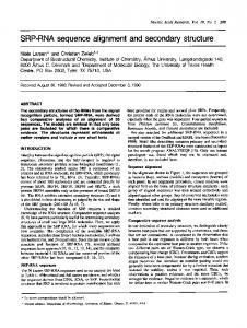
Figure 1.1: Exemplary chemical structure of an RNA double strand.

adenine (A), cytosine (C), guanine (G), and uracil (U). The sugars are joined together by the phosphate groups that form phosphodiester bonds between the third and fifth carbon atoms of adjacent sugar rings. By these asymmetry, a direction is given to the RNA strand, which is always specified in 5’ to 3’ direction (see Figure 1.1). In contrast to DNA (deoxyribonucleic acid), which is composed of two strands and organized in a double helix, RNA consists of just a single strand. But equally to DNA, RNA can form hydrogen bonds between complementary bases according to Watson and Crick [WC53] (A and U, C and G, see Figure 1.1). In some cases, wobble pairings (G and U), or other non-canonical ones can be found. This arrangement of two nucleotides binding together is called a base pair. Contrary to DNA, base pairing usually occurs between bases of the same strand.

4

Chapter 1: Introduction and Fundamental Concepts Definition 1.1.1 (Set of Base Pairs) P BP The set of base pairs is given by = {A-U, U-A, C-G, G-C, G-U, U-G}.

1.1.1

Primary Structure

The simplest way to describe an RNA is just to specify the sequential order of its bases. As already mentioned, bases are given from 5’ end to 3’ end. Definition 1.1.2 (Set of Bases) PB The four element set of bases is given by = {A, C, G, U}.

Definition 1.1.3 (Primary Structure, Primary Sequence) P The sequence S = S1 ...Sn of n bases Si , where 1 ≤ i ≤ n and Si ∈ B , is called the primary structure or the (primary) sequence of the RNA. Exemplarily, the primary structure of the yeast phenylalanine tRNA (tRNAPhe ) can be given by 5’-GCGGAUUUAGCUCAGUUGGGAGAGCGCCAGACUGAAGAUCUGGAGGUCCUGUGUUCGAUCCACAG AAUUCGCACCA-3’

1.1.2

Secondary Structure

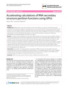
The activity of RNA is determined by its structure, the way it folds back on itself. The structure that arises after forming hydrogen bonds between bases of an RNA is called the secondary structure of that RNA. It is determined as the set of WatsonCrick, wobble, and other (non-canonical) base pairings that form when the RNA is folded. Here, we define a non-canonical base pair as non-Watson-Crick and non-wobble pair. Definition 1.1.4 (Secondary Structure) The secondary structure of an RNA sequence S = S1 ...Sn is defined as a set T = {(Si , Sj )|1 ≤ i < j ≤ n; Si and Sj pair} of base pairs between nucleotides. (Si , Sj ) or in short (i, j) denotes the base pair between the nucleotides Si and Sj . Each nucleotide can at most pair with one other nucleotide. Thus, two base pairs (i, j) and (k, l) are either identical (i = k and j = l) or differ in both nucleotides (i 6= k and j 6= l). As an example, the secondary structure of the yeast tRNAPhe is shown in Figure 1.2. Definition 1.1.5 (pseudoknot-free) An RNA secondary structure T is called pseudoknot-free if for every two base pairs (i, j) and (i′ , j ′ ) in T with i < i′ holds i < j < i′ < j ′ or i < i′ < j ′ < j.

1.1 Different Views at RNA and its Structure

D loop

U

G

A

U G G

G

A

CUCG GA G C

A

G

3’ A C C A C acceptor stem G C U U A T loop U A C A G AC A C

5’ G C G G A U U U

C C A G A

C U G

5

A

G CUGUG C U CU U G variable loop G AG G U C anticodon loop U A G A

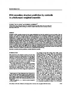
Figure 1.2: Secondary structure of yeast tRNAPhe [JDR00]. Possible pseudoknots are shown in Figure 1.3. If such constructs would be taken into account, the loop decomposition (explained in the following) as well as the energy rules described in Section 1.3 break down. Thus in the following, all regarded secondary structures are pseudoknot-free. They are also called nested structures. Definition 1.1.6 (Accessibility [ZMT99]) A base pair (i′ , j ′ ) is called accessible from a base pair (i, j) if i < i′ < j ′ < j and if there is no other base pair (k, l) such that i < k < i′ < j ′ < l < j. Likewise, a free base i′ is called accessible from a base pair (i, j) if i < i′ < j and if there is no other base pair (k, l) such that i < k < i′ < l < j.

H−type pseudoknot

kissing hairpins

3’

5’

5’

Figure 1.3: Exemplary pseudoknots.

3’

6

Chapter 1: Introduction and Fundamental Concepts Definition 1.1.7 (Loop, Loop Closing, Loop Inclusion [ZMT99]) The collection of bases and base pairs accessible from a base pair (i, j), but not including that base pair, is called the loop closed by (i, j). All accessible pairs and bases are also called included in the loop. Definition 1.1.8 (Loop Size) The number of free bases included in a loop is also named the size of the loop. Secondary structures can be decomposed into loops. They represent the smallest structural entities and are also called structural elements in the following. Depending on the number of included base pairs and free bases, we distinguish between different types of loops. Definition 1.1.9 (Structural Elements) The structural elements a secondary structure consists of can be described as follows: • A hairpin loop (HL) is a loop including only free bases and no base pair. Since sharp U-turns in an RNA secondary structure are prohibited for steric reasons, a hairpin loop must contain at least three bases. • A stacking pair is a loop including only one base pair but no free bases. • An interior loop (IL) includes one base pair and has a size > 0. If all free bases included in the loop are located on one side of the loop, it is called a bulge loop (BL). • A multi-branch loop (ML) (short: multiloop) is a loop including more than one base pair. • All bases and base pairs that are not accessible from any other base pair are called exterior loop (EL). Often, structural elements are summarized and generalized as loops. A visualization of the structural elements is given in Figure 1.4.

1.1.3

Tertiary Structure

For the understanding of catalytic activities of RNA, knowledge of its secondary structure alone is often incomplete. Thus, tertiary (i.e. three dimensional) atom positions and interactions have to be taken into account. As an example, the tertiary structure of the yeast tRNAPhe is given in Figure 1.5. Here, the typical L-shape structure of tRNAs can be seen. The underlying secondary structure is shown in

1.2 RNA Secondary Structure Representations

bulge loop

stacking pair

5’

7

3’

5’

interior loop

3’

5’

3’

hairpin loop

multiloop

5’

3’

5’

3’

Figure 1.4: Structural elements of the RNA secondary structure. Figure 1.2. The tertiary structure forms by additional three dimensional interactions and can be specified by its atomic coordinates. Possible tertiary interactions may include bindings where three bases are involved [LSW02]. For some RNAs, three-dimensional structures could be determined by crystallography. But RNA is hard to crystallize, which is due to their structural flexibility compared to proteins. Furthermore, secondary structure (i.e. the set of canonical and wobble base pairs) is stronger and forms faster than tertiary structure [LTM06, Woo00] and, for the most part, it determines the tertiary structure. The secondary structure can largely be identified without knowing tertiary interactions. Since prediction or experimental determination of three-dimensional RNA structures remain difficult, much work focuses on problems associated with its secondary structure. Hence in the following, we will focus on the secondary structure of RNA.

1.2

RNA Secondary Structure Representations

There are many ways to represent an RNA secondary structure, e.g. as a graph, as a string, as a rooted ordered tree, by a mountain, or a circle representation [MZS+ 00]. Only the first two mentioned are used in this thesis.

8

Chapter 1: Introduction and Fundamental Concepts

Figure 1.5: Tertiary structure of yeast tRNAPhe . Colors are chosen according to Figure 1.2. Definition 1.2.1 (Secondary Structure Graph [Wat78, Hof94]) A secondary structure graph of an RNA sequence of length n is an undirected vertex-labeled graph with n vertices and a symmetric adjacency matrix (A) = ai,j , where 1 ≤ i, j ≤ n, fulfilling the following properties: (1) ai,i+1 = 1 for 1 ≤ i < n (representing the backbone); (2) for each i, 1 ≤ i ≤ n, there is at most a single j ∈ / {i − 1, i + 1} such that ai,j = 1 (representing base pairs). The secondary structure graph of a pseudoknot-free RNA secondary structure also fulfills the following: (3) if ai,j = ak,l = 1 and i < k < j, then i < l < j. Thus, when representing the RNA secondary structure as a graph, each nucleotide is assign to a vertex. All neighbored nucleotides as well as all paired bases are connected by an edge. Figure 1.6A shows a spatial picture of the secondary structure graph, while in Figure 1.6C all vertices are arranged in one line and base pairs are represented by arcs.

1.3 The Energy Model of RNA Secondary Structure

9

The most compact representation of the secondary structure is to display it as a string of brackets and dots. Here, each base pair (i, j) is replaced by a left parenthesis ’(’ and a right one ’)’ at the ith and jth position, respectively. Unpaired bases are represented by a ’.’. This representation is called dot-bracket notation. An example is shown in Figure 1.6B.

1.3

The Energy Model of RNA Secondary Structure

The problem of predicting the secondary structure of a given RNA sequence is called the RNA folding problem. Today, the most common computational approach is based on a thermodynamic model that assigns a free energy value to each secondary structure [Zuk94]. The structure with the lowest possible free energy, the minimum free energy (mfe) structure, is expected to be the most stable secondary structure for a given RNA sequence. In various experimental tests, Douglas H. Turner and colleagues [FKJ+ 86, TSJ+ 87, TS88, JTZ89, MSZT99, LTM06] determined several thermodynamic parameters that can be used for computational prediction of RNA secondary structures. These are also called nearest neighbor energy rules since they assign free energies to loops rather than to single base pairs. Thus, a free energy is assigned to each structural element (as defined in Definition 1.1.9) independently and summed up additively to the free energy e(T |S) of the complete RNA sequence S folded into the RNA secondary structure T , which can be determined by e(T |S) =

X

e(loop)

(1.1)

loop∈T

where e(loop) is the free energy of a structural element. The energy contribution of a structural element depends on its type. Generally, negative stabilizing energies are assigned to stacking base pairs and unpaired bases adjacent to a base pair, whereas destabilizing energies are associated with bulge, interior, hairpin, and multiloops [Zuk94]. The energy contributions of the different structural elements in the model according to Zuker, Mathews, and Turner [ZMT99] are explained in the following. Stacking pair. Free energy values for all 21 possible combinations of two base P pairs from BP were determined experimentally. They do not depend on anything else. A group of two or more consecutive base pairs is called a helix.

10


A) 3’ 5’

B)

5’ ..(((((((.((...))))).((((.(((....)))..))))..)))). 3’ C)

5’

3’

Figure 1.6: Different representations of an RNA secondary structure used in this thesis. A) shows the widely used representation as secondary structure graph. Vertex labels are left out for clarity reasons. B) represents the structure in dotbracket notation. C) displays another version of the RNA secondary structure graph shown in (A).

1.3 The Energy Model of RNA Secondary Structure The energy contributions of all kinds of loops (HL, BL, IL, EL, and ML) have in common that they ignore the assignments of the unbound bases included in the loops (except for unbound bases adjacent to included or closing base pairs of the loops). This is due to the current inability to quantify these effects experimentally. Thus, they are estimated by the number of free bases in the loops in order to predict the stability of any possible sequence [MSZT99]. Hairpin loop. The free energy contribution of a HL depends on three terms: 1. a size-dependent parameter, 2. for loops of a size larger than three, a hairpin loop terminal stacking energy is added due to the interaction between the closing pair and both adjacent unpaired bases, and 3. for specific tetraloops (HLs of size four), special bonus energies are added. Bulge loop. Free energies for BLs depend basically on the loop size. Furthermore for bulge loops of size one, the stacking contribution of the closing base pair and the pair included in the loop is added. Interior loop. Similarly to the hairpin loop, the free energy fraction of an IL depends on three items: 1. a size-dependent value, 2. interior loop terminal stacking energies are added for all unpaired bases adjacent to the closing pair and to the included pair, respectively, and 3. an asymmetric loop penalty is added for interior loops if the left loop size differs from the right loop size. Exterior loop. The only free energy contribution of an EL arises from free bases in the loop that are adjacent to base pairs of the loop. This fraction is called dangling base energy. If a free base is adjacent to two base pairs, the favorable (i.e. smaller) dangling base energy is added. Free bases that are not adjacent to a base pair do not contribute to the energy. Multiloop. Basically, the energy fraction of a multiloop is determined by a term eML (s, f ) that depends on the number of free bases f in the multiloop as well as on the number of stems s that originate from the loop (i.e. included base pairs) plus the closing pair [ZMT99]. The following equation gives an estimation of this

11

12

Chapter 1: Introduction and Fundamental Concepts energy fraction, which was also made due to the current inability of quantifying these effects experimentally depending on any possible assignment of the bases. eML (s, f ) = a + b ∗ f + c ∗ (s + 1)

(1.2)

where a, b, and c are constants representing an offset, a free base penalty, and a helix penalty, respectively. Additionally, dangling base energies have to be added similar to exterior loops. Furthermore, we distinguish between GC and non-GC closing base pairs. A penalty (called terminal AU penalty) is assigned to all non-GC closing pairs at the end of a helix or a hairpin loop of size three (called triloop). This penalty is also added in case of included and closing non-GC pairs of bulge loops of sizes larger than one. Widely used folding algorithms applying these energy parameters are based on dynamic programming and find a nested structure having minimum free energy within O(n4 ) time (given a sequence of length n) [ZS81, LZP99]. The most frequently used implementations are mfold [Zuk94, Zuk03] and RNAfold [HFS+ 94]. They restrict the maximal size of interior loops and thus find the minimum free energy within O(n3 ) time. Even if various experimental data are available for parameterization nowadays, they might still be not precise enough. Small changes in energy parameters can result in large changes in predicted foldings. Thus, the problem is ’ill-conditioned’ in a mathematical sense [ZJT91]. Furthermore, it is not clear whether the real RNA molecule folds to the structure having the lowest free energy or to a different one that has slightly higher energy. Indeed, the real biological structure is often contained in the set of few suboptimal structures. This might happen if the RNA molecule traps in a local minimum of the energy landscape during the folding process. Therefore, kinetic folding algorithms try to simulate the folding process [Mar84, MDK85, FFHS00]. Additionally to the thermodynamic and the kinetic approaches, which are both energy directed, RNA secondary structure can be predicted by phylogenetic comparison. Here, a large number of sequences having similar secondary structures is needed. They must neither be to similar nor to divergent [Hof94]. The most prominent strategies are (i) the generation of a multiple sequence alignment and a subsequent determination of the consensus secondary structure inferred from the evolutionary and energetic information contained in the alignment and (ii) the simultaneous identification of the alignment and the consensus structure (called the ’Sankoff algorithm’) [San85, HBS04, GG04, WRH+ 07].

1.3 The Energy Model of RNA Secondary Structure In recent years, further phylogenetic methods were developed. Stochastic contextfree grammars (SCFGs) have been shown to be a possible methodology for modeling of RNA structure [KH99, KH03]. Nevertheless, the best energy-directed methods perform still better than the best SCFG-orientated approaches [DE04]. In 2006, CONTRAfold, a new secondary structure prediction tool using a flexible probabilistic model called conditional log-linear model (CLLM), was introduced. CLLMs incorporate both; the computational parameter learning of SCFGs and some complex scoring schemes used in energy-based structure prediction. Using CONTRAfold, the authors obtained the highest single sequence prediction accuracies to date [DWB06]. However, the thermodynamic approach of finding the structure having the lowest free energy is widely used. This is due to its usability without knowing any other sequences and structures. The only required prior knowledge is the set of energy parameters previously determined by Douglas H. Turner and colleagues [FKJ+ 86, TSJ+ 87, TS88, JTZ89, MSZT99, LTM06]. Furthermore by using the thermodynamic approach, one can calculate the partition function of a sequence and its ensemble of possible structures [McC90], which is not possible with other secondary structure prediction approaches. Additionally, the probability of each structure can be determined based on the partition function. In the following, all introduced algorithms are based on the thermodynamic model introduced in this section. Its additive decomposition is its main advantage and the reason why we are using it. All used energy parameters are downloaded from Michael Zuker’s homepage on http://frontend.bioinfo.rpi.edu/zukerm/cgi-bin/efiles-3.0.cgi.

13

14


Chapter 2 RNA Design - The Inverse Folding of RNA 2.1

Biological Introduction and Importance of the Problem

Since the function of RNA molecules depends crucially on their structure, the design of RNAs having special structural properties is of interest for biologists in several fields. RNA molecules that catalyze others are called ribozymes. They are involved in the regulation of RNAs, most commonly in the cleavage of an RNA or DNA strand. Here, the group I self-splicing introns are a widely known example. The cleavage at the correct site requires a special RNA secondary structure [DS89, Cec92]. Other described ribozymes are the self-cleaving hammerhead and hairpin ribozymes and the trans-cleaving ribonuclease P (RNase P). The latter is involved in the processing of tRNAs, while the former two are involved in gene control [SP07]. This catalytic variety of RNA opens the question of the design of new ribozymes with possibly new catalytic functions. Speaking of RNA design, we always refer to the design of an RNA sequence that folds into a functional structure. The design of new ribozymes may support the design of drugs and human therapeutic agents, respectively [UM95]. For example, the production of better agents for the inhibition of gene expression might be used to understand biology or for pharmaceutical applications. Several ribozymes have a catalytic core that assures their activities. Thus, RNA design may help to define the minimum structural requirements for catalysis [DS89, BJ90, Cec92]. Developing new systems with increasing functional density requires the understanding of the design of molecular structures. For the construction of nanoscale devices with novel mechanical or chemical functions, nucleic acids seem to be an excellent medium [DLWP04].

16

Chapter 2: RNA Design - The Inverse Folding of RNA Finally, the design of RNA molecules having special functions can facilate the research on the function of natural occurring RNAs [AFH+ 04]. It may help to understand the mechanisms of catalysis and principles of RNA folding [Cec92] and allows to predict novel sequences that are functionally equivalent but unrelated to naturally occurring RNAs [Hof94]. Based on all these findings, here, we consider the inverse RNA folding problem, which is the design of RNA sequences that fold into a desired structure. Apart from its application to ribozymes and riboswitches [Kni03, WNR+ 04, Cec04] mentioned above, it can be applied to the design of non-coding RNAs, which are involved in a large variety of processes, e.g. gene regulation, chromosome replication, and RNA modification [Sto02]. Furthermore, the inverse RNA folding allows the design of cis-acting mRNA elements such as the iron responsive element (IRE) and the polyadenylation inhibition element (PIE). Both elements have a conserved secondary structure and few conserved sequence positions in loops. By providing binding sites for regulatory proteins, they determine mRNA stability and translation efficiency. The IRE is essential for the expression of proteins that are involved in the iron metabolism [HK96]. The PIE contains two binding sites for U1A proteins [VGM+ 00]. U1A binding leads to an inhibition of the poly(A) polymerase and a reduced mRNA stability and translation efficiency due to a shortened poly(A) tail.

2.2

Existing Approaches and their Limitations

Given an RNA secondary structure, we aim at finding an RNA sequence that adopts this structure. Only compatible sequences (see Definition 2.3.2) are considered as candidates in the inverse folding procedure. Clearly, a compatible sequence can but need not have the target structure as its minimum free energy (mfe) structure. It is impossible to test each compatible sequence, whether its mfe structure is the searched one, since the number of sequences grows exponentially in the size of the structure [Hof94]. The exact complexity of the design problem is unknown, in particular it is not known whether a provable efficient (i.e. polynomial-time) algorithm exists for the inverse RNA folding problem [AFH+ 04, AHHC07]. Thus, different heuristic local search strategies, which do not analyze the complete solution space, were used by existing programs dealing with inverse RNA folding. Nevertheless, there are only few publications that address the inverse RNA folding problem, e.g. [Hof94, AFH+ 04, DLWP04]. One approach is implemented in RNAinverse, which is included in the Vienna RNA Package [Hof94]. They use the

2.2 Existing Approaches and their Limitations strategy of adaptive walk and find local optima concerning a structure distance between the mfe structure of the designed sequence and the target structure (mfemode), or concerning the probability of folding into the target structure (p-mode). During the adaptive walk, RNAinverse starts with a random sequence and finds new candidate sequences by iteratively modifying single unpaired bases or base pairs in order to find a sequence that fits better their optimization criterion (structure distance or probability). As soon as they have found a better sequence, the modified position(s) are mutated and the search for better candidates continues. It stops, if a solution is found (a sequence whose mfe structure is the target one) or no modification provides a better candidate, which means, that the search is stuck in a local optimum. During the mfe-mode, the adaptive walk is done recursively since substructures contribute additively to the energy. Small substructures are optimized first and proceeded to larger ones. RNAinverse acts very well, if we consider short structures (up to 200 bases). But for larger structures, it is quite slow and maximizing the probability of folding into the target structure does not work anymore since the adaptive walk is not done recursively during p-mode. There, the optimization is done on the whole sequence and thus, too much computation time is needed. Using RNAinverse, Schuster et al. [SFSH94] derived some thousand sequences for several structures. They found that their pairwise sequence distances are not distinguishable from the distances of random sequences compatible with the given structure. This finding supports the hypothesis that sequences folding into the same structure are randomly distributed in the sequences space and thus, there is no need to search large fractions of the sequence space to find a sequence folding into the given structure. They further stated that the average number of mutations, which are needed to convert a random compatible sequence into one that folds into the target structure, is much smaller than the sequence length. In contrast, Andronescu et al. [AFH+ 04] as well as ourselves [BB06] found several structures that are hard to design independent of their sizes. These findings support the difficulties in finding the correct complexity of the design problem. Dirks et al. [DLWP04] have also used an adaptive walk to analyze several objective functions (values to be optimized) and compared them to each other. They found out that (in case of adaptive walk) the most successful objective functions are maximizing the probability of folding into the desired structure and the newly introduced function of minimizing the average number of incorrect paired nucleotides. Unfortunately, they gave no hint concerning time needed to compute the solutions.

17

18

Chapter 2: RNA Design - The Inverse Folding of RNA Furthermore, Andronescu et al. [AFH+ 04] have developed an algorithm called RNA-SSD (RNA Secondary Structure Designer). It is based on a recursive stochastic local search, which tries to minimize a structure distance of the target structure and the mfe structure of the designed sequence. RNA-SSD also uses the fold functions of the Vienna RNA Package. In a first step, RNA-SSD creates a starting sequence whose mfe structure is close to the target one. To do so, RNA-SSD uses different probabilistic models for paired and unpaired positions when assigning bases randomly to the sequence. Furthermore, their algorithm avoids complementary stretches of bases except they are desired along two sides of a stem [AFH+ 04]. During a second step, they use a hierarchical decomposition of the structure into smaller substructures to reduce the complexity of the problem. Then, they apply a stochastic local search (SLS) to the smallest substructures and finally combine them to larger ones. Similar to the adaptive walk, the SLS finds new candidate strands by iteratively modifying single unpaired bases or base pairs. The modified position(s) are mutated if a better sequence is found. If the candidate sequence has a worse value concerning the objective function, it is mutated with a low probability. The search is stopped, if a solution is found (a sequence whose mfe structure is the target one) or a maximum number of mutations is done. RNA-SSD is available online, but the size of the input structures is restricted to 500 there. Using an advanced version of RNA-SSD, Aguirre-Hernández et al. [AHHC07] propose that the empirical time-complexity of the RNA design problem is polynomial. They estimated a median expected run-time of about O(n3 ) for RNA-SSD and of about O(n5 ) for RNAinverse, where n is the size of the structure. Westhof et al. [WMJ96] proposed the construction of a combinatorial library consisting of modular units, which can be used for the creation of new RNA molecules with a given structure. This approach is based on the hierarchical organization of the folding process, i.e. secondary structure elements form first while tertiary contacts are composed afterwards. According to our experiments, constructing RNA sequences from small units is not successful in most cases (data not shown).

2.3

A New Approach: INFO-RNA

Here, we present a new algorithm for the design of RNA sequences that fold into a given structure. Since the problem of finding the secondary structure of a given RNA sequence is called the RNA folding problem, the inverted case is called the inverse RNA folding problem. Formally, it can be defined as follows.

2.3 A New Approach: INFO-RNA Definition 2.3.1 (Inverse RNA Folding) The inverse folding of RNA is the problem of finding an RNA sequence S = P S1 ...Sn of length n that folds into a given secondary structure T , where Si ∈ B = {A, C, G, U} for 1 ≤ i ≤ n. T can be described as a set of pairs as defined in Section 1.1.2. Definition 2.3.2 (Compatible Sequence) A sequence is called compatible to a given structure, if it can form all required base pairs regardless of energy. The set of all compatible sequences is called S. To find the best sequence that folds into a given structure, a search space of an exponentially high number of compatible RNA sequences has to be analyzed. Therefore, it takes exponential time to find a globally optimal solution by testing all candidate sequences and thus, local search methods are widely used to address the inverse folding problem. Consequently, the resulting local optima are not guaranteed to be globally optimal but are optimal among all their sequence neighbors. Definition 2.3.3 (Sequence Neighbor) All compatible sequences that differ from a sequence S in one unbound position or in two positions, which have to pair in structure T , are called sequence neighbors of sequence S (see Figure 2.1). We introduce a new algorithm INFO-RNA attending the INverse FOlding of RNA. It consists of two steps; a new design method for good initial sequences and a following improved stochastic local search that uses an effective neighbor selection method. Except on the search strategy itself, the performance of the local search depends on the quality of the initializing sequence. Often, it is chosen at random. We found that a good choice is to use a sequence that among all sequences adopts the given structure with the lowest possible energy. We present a dynamic programming approach to solve this problem. Here, multi-branched loops are especially complicated to handle. In the following, we introduce the new method to create an excellent initializing sequence and describe the subsequent local search strategy.

2.3.1

The Initializing Step

The initializing step of INFO-RNA uses the technique of dynamic programming. This method was successfully applied to RNA secondary structure prediction as mentioned in Section 1.3 [ZS81] and related problems. Similar to Zuker and Stiegler [ZS81], we use free energies of structural elements [stacks, bulge- (BL), interior- (IL), hairpin- (HL), multiloops (ML)] as defined in Section 1.3. They

19

UA

CC

AAUACCAUU

AGU A CC A UU U AU C AC U

AG UC

AG

GC

AGUAC CACU UA CC AA U

Chapter 2: RNA Design - The Inverse Folding of RNA

AU

20

G

UAC

A

AC

CAG

U CAGA

U

ACGACCUG ACUACCAGU ((( ... )))

GCUACCAGC

ACUACCGGU

ACGAC

AGG

ACC

A

ACUCCCAGU

U GU

AG

GC CA

AC

ACU

UA AC

A

AGU

UA

CG

U AG CA UA AGU AC UCC AC U

C

G

A CU

ACU

AC

U

AG

A

CCGU

ACU

GU

UC

A CU

GU

CG

AC ACC

UCUAC

CCU

U

UG

C AC

AG

U

Figure 2.1: Exemplary sequence (and structure) and all its sequence neighbors that can adopt this structure. The dot-bracket notation is used for the representation of the RNA secondary structure. depend on the size of the loop, the closing and included base pairs, as well as on the free bases inside the loops that are adjacent to the closing and included pairs. Free bases that are not adjacent to a base pair do not give any energy fraction. Since each pair belongs to two elements, neighbored elements in a structure are linked and base pairs cannot be handled independently. The free energy value of a pseudoknot-free structure is calculated by adding up all partial energies of its elements (see Equation 1.1). Given a target structure T , we find among all sequences a sequence S that adopts T with the lowest possible energy. Formally, this means that we find a sequence S resulting from argmin e(T |S ′ )

(2.1)

S′

where e(T |S ′ ) represents the free energy of sequence S ′ folded into structure T . For solving this problem, our dynamic programming algorithm needs linear time depending on the structure size. It divides the target structure into its structural

2.3 A New Approach: INFO-RNA elements. Before explaining the algorithm, some formal definitions concerning the structural elements and the ordering of the base pairs are needed. Definition 2.3.4 (Substructure) A substructure T(i1 ,i2 ) of structure T is defined as a structural part of T that is closed by pair (i1 , i2 ) and has a connected backbone (see Figure 2.2B). e(T(i1 ,i2 ) |(Si1 , Si2 ) → (a1 , a2 )) is defined to be its minimum free energy under the condition that the sequence positions (Si1 , Si2 ) of the closing pair (i1 , i2 ) of the substructure are fixed to a base pair assignment (a1 , a2 ). In the following, we will give a formal definition of a structural element, which was already introduced in Section 1.1.2 (Definition 1.1.9) in a more descriptive and informal way. Definition 2.3.5 (Structural Element) (·,·)...(·,·) T(i1 ,i2 ) indicates a structural element of structure T that is closed by the pair given in the subscript (i1 , i2 ) and includes all base pairs indicated in the superscript. The structural element does not need to have a connected backbone (see Figure 2.2C). (j ,j )...(p ,p )

e(T(i11,i22) 1 2 |(Si1 , Si2 ) → (a1 , a2 ), (Sj1 , Sj2 ) → (b1 , b2 ), ..., (Sp1 , Sp2 ) → (r1 , r2 )) is defined as the minimum free energy of the structural element that is closed by base pair (i1 , i2 ) and includes pairs (j1 , j2 ),...,(p1 , p2 ), whose sequence positions are fixed to assignments (a1 , a2 ), (b1 , b2 ), ..., and (r1 , r2 ), respectively. Note, that we will use the following conventions: • In case of a stack, a BL, or an IL, the structural element includes exactly one base pair and is closed by exactly one pair. Thus, one pair is indicated in the subscript and in the superscript, respectively. • In case of a ML, the structural element includes more than one base pair, whose are indicated in the superscript. • In case of an EL, the structural element has no closing pair and thus an empty subscript. • In case of a HL, the structural element has no included pair and thus an empty superscript. Therefore, a HL can also be interpreted as a substructure. Furthermore, we have to define an order ≺ of the base pairs in the structure. It specifies the order in which base pairs are analyzed during the initializing step of INFO-RNA.

21

22


A) 18

B)

19

30

17

20 16

21

15

22 23

13 14 9 10 11 12

29 24 29 25 26 27 28

8

31

28 27

32 33

26

35

27

33

26

35

34

30 7

6 5 4 3 2 1

36 38 39

37

35

33 32 34

31

C) 34

Figure 2.2: A) RNA secondary structure, B) Substructure T(26,35) having a con(27,33)

nected backbone, C) Structural element T(26,35) without a connected backbone Definition 2.3.6 (Base Pair Order) All base pairs of a structure T are analyzed in a predefined order ≺, where (i1 , i2 ) ≺ (j1 , j2 ) means that base pair (i1 , i2 ) is analyzed prior to base pair (j1 , j2 ). The actual order in which the base pairs are examined is defined as follows. (i1 , i2 ) ≺ (j1 , j2 ) if and only if

i1 > j1

(2.2)

Relating to the example of Figure 2.2A, the order of all pairs is the following: (28, 32) ≺ (27, 33) ≺ (26, 35) ≺ (25, 36) ≺ (16, 21) ≺ (15, 22) ≺ (14, 23) ≺ (6, 10) ≺ (5, 11) ≺ (4, 12) ≺ (2, 38) ≺ (1, 39). Notation 2.3.7 (Predecessor) According to the definition of the order, all base pairs accessible from a fixed pair are smaller than itself and thus called its predecessors. Since closing pairs of HLs have no accessible base pairs, they have no predecessor. The closing pair of a ML has as many predecessors as accessible base pairs. All other pairs have exactly one predecessor. Table 2.1 shows the predecessors of Figure 2.2A.

2.3 A New Approach: INFO-RNA

base pair

predecessor(s)

(28, 32) (27, 33) (26, 35) (25, 36)

none (28, 32) (27, 33) (26, 35)

(16, 21) (15, 22) (14, 23)

none (16, 21) (15, 22)

(6, 10) (5, 11) (4, 12)

none (6, 10) (5, 11)

(2, 38) (1, 39)

(4, 12), (14, 23), (25, 36) (2, 38)

Table 2.1: Base pairs and their predecessors in the structure of Figure 2.2A.

Idea. The basic idea of the initializing step of INFO-RNA is to start with small substructures and enlarge them gradually by one base pair. Thus, the algorithm starts at the closing pair of P a hairpin loop, subsequently fixes it to pair assignments out of the set of valid pairs BP = {A-U, U-A, C-G, G-C, G-U, U-G}, and assigns the unbound positions of the loop such that they provide the lowest possible free energy value for this small substructure under the condition that the closing pair is fixed. This is stored for all six possible assignments of the pair. Afterwards, the next pair to the HL-closing one is fixed. The energy can be calculated by the sum of the energy of the hairpin loop including the closing pair and the stacking energy of the current pair and the closing one of the HL. To find the best energy value, we have to minimize this sum over all possible assignments of the base pair closing the HL. This is demonstrated in Equation 2.3 exemplarily, where e(.) represents the minimal free energy. The substructures refer to Figure 2.2A.

23

24




 e

18

19

17

20 16

A15

21

U22



  = min

    e                e                 e    

18

19

17

20

A16

18

U21

19

17

20

U16

18

A 21

19

17

20

C16

      e                 e                 e

18

G 21

19

17

20

G16

18

C21

19

17

20

G16

18 17

U21

19 20

U16

G 21

! ! ! ! ! !

+e

+e

+e

+e

+e

+e

A16

U21

A15

U22

U16

A21

A15

U22

C16

G21

A15

U22

G16

C21

A15

U22

G16

U21

A15

U22

U16

G21

A15

U22

                                      

(2.3)

                                     

Equation 2.4 formalizes the example of Equation 2.3.

e

T(15,22) (S15 , S22 ) → (A, U)

min

   

(a1 ,a2 )  



e

=

T(16,21) (S16 , S21 ) → (a1 , a2 )

e +

(16,21)

T(15,22)

(S16 , S21 ) → (a1 , a2 ) (S15 , S22 ) → (A, U)

   

(2.4)

  

Generally, the energy value of any structural element depends on the assignment of the base pairs and, in case of a loop, on the included unpaired bases adjacent to the pairs and on the loop size. The minimal energy of a substructure T(i1 ,i2 )


base pair

1

2

25

3

4

5

6

A−U U−A C−G G−C G−U U−G

...

1 2 3 4

Figure 2.3: Dynamic programming matrix D can be evaluated by adding the minimum energy of the one pair smaller substruc(i +k,i −l) ture T(i1 +k,i2 −l) and the energy of the structural element T(i11,i2 ) 2 . Therefore, an already analyzed smaller substructure can be seen as black box, except for its closing pair. We calculate the lowest possible energies for substructures gradually by adding the next pair to a smaller substructure. In case of a ML, as many smaller substructures as included pairs are in the loop have to be added. Having set the order of the pairs, a dynamic programming matrix D is filled with minimal free energies. Each row in D represents a base pair of the target structure while each column stands for a possible assignment of the base pairs (see Figure 2.3). Thus, D has as many rows as pairs are in our desired structure and six columns, which represent the assignments A-U, U-A, C-G, G-C, G-U, and U-G. The rows are sorted according to ≺. In the following, pairs are no longer represented by their pairing positions, e.g. (i1 , i2 ), but only by their row numbers in D. The values in the matrix D(i, a) give the minimal free energy of a substructure ending at base pair i (represented by the row) P that is assigned to a ∈ BP (given by the column). Every substructure starts at one or more base pairs that do not have any predecessors. Before giving a detailed description of the algorithm, we have to define some variables and notations that are used in the following equations. Now, Tij represents the structural element of T closed by base pair i and including base pair j, where i and j are row numbers in D. The free energy of this structural element when i and j j are assigned to a and b, respectively, is given by e Ti i → a, j → b . Further definitions are shown in Table 2.2.

26


pk (i)

k-th predecessor of pair i (sorted according to the order)

s

number of stems originating from a ML (= number of predecessors of the closing base pair of the ML)

F

number of free bases adjacent to stems in a ML

f

total number of free bases in a ML

eML (s, f )

size-dependent energy fraction of a ML with f free bases and s stems. It equals a + b ∗ f + c ∗ (s + 1), where a, b, and c are constants (see Equation 1.2).

edb (b)

dangling base energy of a free base assigned to b and adjacent to one or two stems in a ML or an EL

H

total number of free bases in a HL

eHL (H)

size-dependent energy fraction of a HL of size H

ebonus a,b1 ,...,bH

HL bonus energy depending on the assignments a and b1 , ..., bH of the closing pair and the free bases, respectively. It is lower than 0 for some special tetra HLs. Otherwise it is set to 0.

eTM (a, b1 , bH )

terminal stacking and mismatch energy in HLs. It depends on the assignment a of the closing pair of the HL and the assignment of the directly adjacent free bases b1 and bH .

eAU (i, a)

terminal AU penalty. It penalizes stems, whose last pair is assigned to A and U or G and U. The same holds for base pairs that close a triloop and for base pairs included in or closing a BL of size larger than one.  0.5 if i is the last pair of a stem, the     closing pair of a triloop, or included  in or closing a BL of size > 1 eAU (i, a) =   and a ∈ {A-U,U-A,G-U,U-G}    0 otherwise to be continued on the next page

Table 2.2: Definition of additional terms used during the initializing step of INFORNA.


27

continuation of the previous page Ll , Lr

left and right size of an IL or BL, respectively

easym (i − 1, i)

asymmetric loop penalty that is added for ILs if Ll 6= Lr . Some exceptions for small nearly symmetric loops exist. easym (i − 1, i) =  0 if (Ll = 0) OR (Lr = 0)     OR (Ll = 1 AND Lr = 2)  l r = OR (L = 2 AND L = 1)   3.0,   otherwise  min 0.5 ∗ Ll − Lr

Table 2.2: Definition of additional terms used during the initializing step of INFORNA. During our dynamic programming approach, the fields in the matrix are filled row by row. Recall that the rows of D are sorted according to ≺. Thus, each pair i has as many predecessors as the structural element closed by i has included pairs. To compute the entries of D, we distinguish between (A) base pairs having no predecessor (closing base pairs of HLs), (B) base pairs with exactly one predecessor (closing pairs of BLs, ILs, or stacks), and (C) base pairs with more than one predecessor (closing base pairs of MLs). (A) If base pair i has no predecessor, i.e. it is a closing pair of a hairpin loop, ∀a ∈

PBP

:

D(i, a) = eHL (H) +

min P b1 ,...,bH ∈ B

(

ebonus a,b1 ,...,bH +

(

eAU (i, a)

,H = 3

eTM (a, b1 , bH ) , H > 3

) )

where the minimum is taken over all possible assignments of all free bases b1 , ..., bH in the HL.

28

Chapter 2: RNA Design - The Inverse Folding of RNA (B) If base pair i has exactly one predecessor, i.e. it is a closing pair of a bulge loop, of an interior loop, or of a stack, ∀a ∈

PBP

:

D(i, a) = eAU (i, a) + easym (i − 1, i)+

+ min P b∈

BP

   D(i − 1, b) +

min

assignment of free bases in Tii−1 that are adjacent to i − 1 or i

 

e

i→a i−1→ b

Tii−1

    

i→a gives the free energy of the structural element bewhere e i−1 →b tween pairs i − 1 and i assigned to a and b. This energy value depends on a and b as well as on the assignment of the free bases directly adjacent to i − 1 and i. Thus, two dependencies can be seen here: the dependency of the base pairs to each other and the dependency to the adjacent free bases.

Tii−1

(C) If base pair i has more than one predecessor, i.e. it is a closing pair of a multiloop, ∀a ∈

PBP

:

D(i, a) = eML (s, f ) + eAU (i, a)+ (2.5) +

min P a1 , ..., as ∈ BP P b1 , ..., bF ∈ B

(

s X k=1

D(pk (i), ak ) +

F X j=1

edb (bj )

)

where the minimum is taken over all possible assignments of all predecessor base pairs a1 , ..., as and of all free bases b1 , ..., bF adjacent to them. At first glance, this evaluation can be exponential in the number of stems originating from the ML and the number of adjacent free bases since the energy fraction of a free base adjacent to two stems depends on the assignments of both. However in nature, MLs have only a low number of stems. Thus, even the naive solution is usable in pratice.

2.3 A New Approach: INFO-RNA To reduce this complexity to linear time for all MLs, we introduce a further dynamic programming matrix M resized and recalculated for each ML. It calculates the best free energy of the substructure closed by the closing pair of the ML dynamically. The evaluation of the ML starts with the first included pair according to the order of the pairs. Here, included base pairs are renumbered starting with 1 being the first included pair. Furthermore, the order is defined as given in Equation 2.2, but the definition of the predecessors is renewed. Definition 2.3.8 (Predecessor in a ML) Now, pair i included in a ML is predecessor to pair j of the ML iff i ≺ j and if there is no other pair k in the ML such that i ≺ k ≺ j. The closing pair of the ML is a predecessor of the first included base pair, while the last included base pair is a predecessor of the closing pair. Matrix M is arranged analogously to matrix D. It has a row for each included base pair of the ML but not for the closing pair. Thus, M has as many rows as there are included pairs in the multiloop. Each column of M represents a possible assignment of the pairs, i.e. M has six columns incorporating A-U, U-A, C-G, G-C, G-U, and U-G. Hence, M(j, a) gives the minimum free energy fraction of the prefix of the ML (and its originating stems) that starts at the first included base pair and ends with the free base adjacent downstream to the j-th included pair, which P is assigned to a ∈ BP . Exemplarily, M(2, a) of the ML in Figure 2.2 gives the minimum free energy fraction of the ML prefix including bases 37, 36, 25, and 24, when base pair (14, 23), which is the second included pair in the ML, is assigned to a. M has to be recalculated for each possible assignment of the closing pair since this base pair is fixed and a predecessor for the first included base pair. In each step, the best energy of the part of the ML is evaluated that includes the current base pair j and all base pairs h with h ≺ j. To this end, all assignments of the previous base pair as well as of the stem-adjacent free base(s) between the current and the previous base pair have to be taken into account. This has to be done, since, firstly, only free bases adjacent to a base pair give an energy fraction and secondly, the energy fraction of a free base depends on the assignment of all adjacent base pairs. Thus, we have to differentiate between the three cases of (I) no, (II) one, and (III) more than one free bases between base pairs in a ML. They are illustrated in Figure 2.4. The respective recursions are given in Equations 2.6, 2.8, and 2.10. There, j represents a base pair included in the ML and its associated assignment is denoted as a.

29

30


stem 1

(II) stem 2

(III) (I) stem 3 Figure 2.4: The three different cases of numbers of free bases between two consecutive base pairs in a ML. (I) corresponds to the first case, where two base pairs are neighbored to each other and thus, no free base is between them (given in blue). (II) contains the most difficult case, where a free base in a ML is adjacent to two base pairs (given in green). In case (III), more than one free bases are between two consecutive base pairs and thus, these free bases are only adjacent to one base pair each (given in red).

Notation 2.3.9 (Dangling Base Energy) The energy fraction of a free base k in a ML or an EL that is • assigned to b, • adjacent to base pair j assigned to a, and • located upstream (up) or downstream (down) of the adjacent base in the adjacent pair db is given by the dangling base energy edb up(b, j, a) and edown(b, j, a), respectively.

(I) If there is no free base between the current base pair j and its predecessor ip, values in M are set according to the following equations.


31

Basic recursive equation of case (I): M(j, a) = min P ap ∈

BP

M(ip , ap ) + D(iD p , ap )

(2.6)

where ap denotes the assignment of base pair ip . While ip indicates the row number in matrix M, iD p represents its respective row number in matrix D. Initialization of case (I): M(1, a) = 0 Final ML recursive equation of case (I): D(i, a) = eML (s, f ) + eAU (i, a) + min P ap ∈

BP

M(ip , ap ) + D(iD p , ap )

(2.7)

where ip indicates the last included base pair of the ML, which is assigned to ap . While ip indicates the row number in matrix M, iD p represents its respective row number in matrix D. Here, i represents the closing pair of the ML according to the base pair numbering of the whole structure. In case of no free base between the last included base pair and the closing pair of the ML, Equation 2.7 replaces Equation 2.5, which is the recursive equation for finding the entry of the closing pair of the ML in matrix D. (II) If there is only one free base between the current base pair j in the ML and its predecessor ip in the ML, values in M can be evaluated using the following equations. Basic recursive equation of case (II): M(j, a) =

min P ap ∈ BP P b∈ B

(

db min{edb down (b, j, a), eup (b, ip , ap )}

+M(ip , ap ) + D(iD p , ap )

)

(2.8)

where ap denotes the assignment of base pair ip . While ip indicates the row number in matrix M, iD p represents its respective row number in matrix D. b represents the assignment of the free base between ip and i.

32

Chapter 2: RNA Design - The Inverse Folding of RNA Initialization of case (II): M(1, a) = min P b∈

B

db min{edb down (b, 1, a), eup (b, ic , ac )}

where ic is the closing pair of the ML, which is assigned to ac . Again, b represents the assignment of the free base between ic and the first included pair in the ML. Final ML recursive equation of case (II): D(i, a) = eML (s, f ) + eAU (i, a)+ +

min P

ap ∈ BP P b∈ B

(

db min{edb down (b, i, a), eup (b, ip , ap )}

+M(ip , ap ) + D(iD p , ap )

)

(2.9)

where ip indicates the last included base pair of the ML, which is assigned to ap . ip indicates the row number in M, iD p gives its respective row number in matrix D. Again, i represents the closing pair of the ML according to the base pair numbering of the whole structure. Once again, b represents the assignment of the free base between the closing pair i and the last included pair ip of the ML. In case of a single free base between the last included base pair and the closing pair of the ML, Equation 2.9 replaces Equation 2.5, which is the recursive equation for finding the entry of the closing pair of the ML in matrix D. (III) If there are more than one free bases between the current base pair j and its predecessor ip, values in M are set according to the following equations. Basic recursive equation of case (III): db eup (bp , ip , ap ) + M(ip , ap ) + D(iD M(j, a) = min p , ap ) P ap ∈ BP P bp ∈ B

db + min P edown (bj , j, a) bj ∈

(2.10)

B

where ap denotes the assignment of base pair ip . ip indicates the row number in M, iD p gives its respective row number in D. bp and bj represent the assignments of the free bases adjacent to ip and to j, respectively.


33

Initialization of case (III): db db M(1, a) = min P eup (bc , ic , ac ) + min P edown (b1 , 1, a) bc ∈

B

b1 ∈

B

where ic is the closing pair of the ML, which is assigned to ac . bc and b1 represent the assignments of the free bases adjacent to the closing pair and the first included pair of the ML, respectively. Final ML recursive equation of case (III): db D(i, a) = eML (s, f ) + eAU (i, a) + min P edown (bi , i, a)+ bi ∈

+

min P

ap ∈ BP P bp ∈ B

B

D edb up (bp , ip , ap ) + M(ip , ap ) + D(ip , ap )

(2.11)

where ip indicates the last included base pair of the ML, which is assigned to ap . Again, ip indicates the row number in M, iD p gives its respective row number in D. Here, i represents the closing pair of the ML according to the base pair numbering of the whole structure. bi and bp represent the assignment of the free bases adjacent to the closing pair i and the last included pair ip of the ML, respectively. In case of more than one free bases between the last included base pair and the closing pair of the ML, Equation 2.11 replaces Equation 2.5, which is the recursive equation for finding the entry of the closing pair of the ML in matrix D. After these steps, we append an additional row to matrix D. It takes into account the dangling base energies of the free bases adjacent to the base pair(s) of the structure included in the EL. Thus, the final free energy of the structure is stored in this additional row. Having filled the complete matrix D, we finally aim at finding the sequence that adopts the given structure with the lowest possible energy. To this end, we choose the smallest energy value of the last row of D. It gives the minimal free energy a sequence can have, when folding into the target structure. To find the sequence that provides this energy, we trace back the matrix D along the path of the best predecessor assignments. For this reason, we store traceback pointers during the computation of D. Finally, all free bases that are not directly adjacent to a base pair and thus do not give any energy value are chosen arbitrarily.

34

Chapter 2: RNA Design - The Inverse Folding of RNA Using this dynamic programming algorithm, we obtain a sequence that among all sequences adopts the target structure with the lowest possible energy. There is no other sequence that has lower energy when folding into this structure. Nevertheless, the sequence is not guaranteed to fold into it since this sequence can have even less energy when folding into another structure. Therefore, the resulting sequence is processed further in a second step presented in the next section. Complexity. During the initializing step of INFO-RNA, we fill matrices D and M and generate the traceback. D has six entries per row and at most n2 many rows, base pairs are since at most n2 base pairs are possible. (To be precise, at most n−3 2 possible since a HL has to include at least three free bases.) Thus, D consists of at most 3n values. Hence, we have to check what time is needed to compute one entry. For that purpose, we differentiate between the three types of entries in D depending on the corresponding base pair (types A, B, or C). For entries corresponding to a closing base pair of a HL (type A), the assignment of all free bases in the loop is only important in case of a tetra-loop. For larger HLs, only the assignment of the free bases adjacent to the closing base pair are taken into account. Therefore, the calculation of a type A entry needs at most 44 steps. During the calculation of values corresponding to pairs having exactly one predecessor (type B), the minima are taken over all assignments of the predecessor and all assignments of the included free bases that are adjacent to the base pairs. Thus, at most 6 ∗ 44 steps are needed. By using the additional dynamic programming matrix M for closing pairs of MLs (type C), all energy values for the closing base pairs of all MLs can be analyzed in at most linear time overall. This is due to the fact that each entry in M can be evaluated in constant time. More precisely, entries of type (I) need at most 6 steps since they are minimized over all assignments of their predecessors. Entries of type (II) can be calculated in at most 6 ∗ 4 steps since all assignments of the predecessor base pair and the free base between the current base pair and its predecessor have to be taken into account. For type (III) entries, at most 6 ∗ 4 + 4 steps are needed. This is due to the fact that all possible assignments of the free base adjacent to the current base pair have to be considered additionally to all possible assignments of the predecessor base pair and its adjacent free base. Each matrix M has to be recalculated for every possible assignment of the closing base pair of the corresponding ML, i.e. each matrix M is calculated 6 times. Even if each ML has its own matrix M, the total number of rows in all matrices M is lower than n2 since each base pair can only be included in a single ML. Thus in total, all matrices M can be calculated in at most linear time, i.e. the

2.3 A New Approach: INFO-RNA evaluation of all type C entries in D needs in total O(n) time. Furthermore, each entry in matrix D of type A or B can be calculated in constant time and hence, evaluating all of them needs O(n) time, too. Consequently, the whole matrix D can be evaluated in linear time as well as the generation of the traceback.

2.3.2

The Local Search Step

After generating the initial sequence as described in the previous section, INFORNA found a sequence S that has the lowest free energy a sequence can have when folding into the desired structure T . However, S is not guaranteed to fold into T because it may have even less free energy when folding into another structure. Therefore, we do a subsequent local search on the sequence. The sequence is mutated iteratively in search of local optimal sequences, i.e. sequences that provide a better value than their neighbored sequences concerning a selected objective or cost function, respectively. Two objective functions applied in INFO-RNA are described in the following. Both of them are used in the Vienna RNA Package [Hof94] as well. Minimum free energy structure distance (mfe-mode). When using a structure distance as objective function, the cost function to be minimized is the structure distance d(T, TS ) between the desired structure T and the minimum free energy structure TS of the designed sequence S. One of the simplest structure distance measures is the base pair distance, which is the minimum number of base pairs that have to be opened or closed in order to convert one structure into the other [Hof94]. A lot of other measures are conceivable (e.g. the Hamming distance, the tree edit distance, the string edit distance, etc.) but as the base pair distance is best suited for our intention (the comparison of different structures on the same sequence) [HFS+ 94], it is used in INFO-RNA. As implemented in the Vienna RNA Package and described in [Hof94], when using the structure distance as objective function, we also use an recursive approach. The optimization starts on small substructures of T instead of working directly on the whole structure. These substructures proceed successively to larger ones. This is done since running the optimization directly on the full length sequence would take too much computation time. The idea is that a substructure, which is optimal for a subsequence, will appear in the full sequence with enhanced probability even if this is not assured. Probability (p-mode). Using the criteria of probability, we try to maximize the probability P (T |S) of sequence S folding into the desired structure T . Again, let e(T ′ |S) be the energy of S folding into structure T ′ . Then the partition function Q(S) of the structure ensemble of S is calculated as sum over the set Ω(S) of all

35

36

Chapter 2: RNA Design - The Inverse Folding of RNA possible secondary structures T ′ of S [McC90]: Q(S) =

X

T ′ ∈Ω(S)

exp(−

e(T ′ |S) ) RTB

where TB is the temperature and R the gas constant given in kcal/mol. Accordingly, the effective free energy G(S) of the Boltzmann ensemble of S is given as

G(S) = −RTB ln Q(S). Thus, we can compute the probability of S folding into T at thermodynamic equilibrium by |S) ) exp(− e(T 1 (e(T |S) − G(S)) e(T |S) RTB P (T |S) = = exp(− exp(− )= ). G(S) Q(S) RTB RTB exp(− RTB )

Therefore, the maximization of this probability can be done by minimizing the cost function c(S) = E(T |S) − G(S) [Hof94]. In combination with the probability criterion, all optimization steps are acting on the full length sequence. Thus, it is not recommended to apply this approach to structures larger than 200. Both optimization criteria (mfe-mode and p-mode) can be used in INFO-RNA. Furthermore, they can be applied one after another. In [DLWP04], Dirks et al. introduced a further optimization criterion. They minimized the average number of incorrectly paired nucleotides w(S), which is described in Section 3.7.1 more detailed. For INFO-RNA, it was not tested successfully and, thus, not further discussed here. Stochastic local search. Apart from the objective function, the success of the local search depends on the search strategy itself. In INFO-RNA, the local search strategy is a stochastic local search (SLS). Today, stochastic local search algorithms belong to the standard methods for solving hard computational problems [Hoo98]. The SLS moves to the first found neighbor of the current sequence that has a better value according to the chosen objective function. To prevent the search from getting stuck in local optima (i.e. sequences that are better than all their neighbors but not necessarily the globally best solution), the SLS is allowed to move to

2.3 A New Approach: INFO-RNA worse neighbors with a fixed probability pw . Thus, a tested neighbor is retained if its value concerning the objective function is better than the value of the current sequence. Otherwise, it is kept with probability pw . The search terminates after a fixed number of steps. We set this number to ten times the length of the structure. As moves to worse neighbors are allowed, the last sequence is not necessarily the best one found. Thus, the best found sequence is stored during the complete search and finally given. As in RNAinverse, we increase the efficiency of the search approach by not taking all sequence neighbors as candidates for mutation. Only sequence neighbors that differ from the current sequence in positions that (a) do not pair correctly and (b) positions adjacent to those are candidates for mutation since they give the best chances of improvement. This is due to the fact that only positions adjacent to a pair give a sequence dependent contribution to the free energy of the structure [Hof94]. In RNAinverse, the classification of the positions is done in the same way. There, not correctly paired positions are tested first and positions adjacent to them afterwards. Within the two groups (a) and (b), candidates are analyzed in an arbitrary order (NA-mode). In contrast, in INFO-RNA the order of testing the neighbors can alternatively be chosen depending on energy with a look-ahead of one selection step (NE-mode) or arbitrarily (NA-mode) as in RNAinverse. In the following, we introduce the new idea of the NE-mode. NE-mode. To use a look-ahead of one selection step, the energy of each candidate sequence folded into the target structure T is calculated. Afterwards, the resulting energy difference to the current sequence folded into T is evaluated. Let e(T |S) be the energy of sequence S folded into the wanted structure T . Let S ′ be a neighbor of S that is compatible to T and that is a candidate for mutation. Let e(T |S ′ ) be the energy of S ′ when folding into T . Then, the energy difference is given by e(T |S) − e(T |S ′ ). The higher the difference is, the earlier the neighbor is examined according to the actual optimization criterion. This pre-selection step can be done easily, since all structural elements contribute additively to the energy of the whole structure and thus, only structural elements that are closed by the mutated pair or include a mutated pair or free base have to be re-evaluated. To evaluate the folding energy, we use functions from the Vienna RNA Package, since it includes the most efficient publically available version of Zuker’s algorithm of which we are aware.

37

38

Chapter 2: RNA Design - The Inverse Folding of RNA Symbol

Set of Nucleotides

A C G U

= = = =

{A} {C} {G} {U}

R Y M K W S

= = = = = =

{A, G} {C, U} {A, C} {G, U} {A, U} {C, G}

H B V D

= = = =

{A, C, U} {C, G, U} {A, C, G} {A, G, U}

N

=

{A, C, G, U}

Origin of designation Adenine Cytosine Guanine Uracil puRine pYrimidine aMino Ketone Weak interaction (2 H bonds) Strong interaction (3 H bonds) not-G, H follows G in the alphabet not-A, B follows A not-U, V follows U not-C, D follows C aNy

Table 2.3: IUPAC symbols for nucleic acids [CB85].

2.4

The Incorporation of Sequence Constraints

Up to now, we concentrated on the constraint-free inverse RNA folding problem. We searched for any RNA sequence that folds into a given structure. Now, we consider the inverse RNA folding problem satisfying sequence constraints, which is the design of RNA sequences that fold into a desired structure and fulfill some given constraints on the primary sequence. Such constraints are important, for example when designing ribozymes or tRNAs since certain base positions must be fixed in order to enable interactions with other molecules.

Definition 2.4.1 (Set of IUPAC Symbols) P IUP AC The set of IUPAC symbols is given by = {A, C, G, U, R, Y, M, K, W, S, H, B, V, D, N}.

2.5 Results Definition 2.4.2 (Inv. RNA Folding Incorp. Sequence Constraints) The inverse RNA folding incorporating sequence constraints is the problem of finding an RNA sequence S = S1 ...Sn of length n that folds into a given secondary structure T and fulfills given constraints C = C1 ...Cn on the primary sequence, P where Ci ∈ IU P AC for 1 ≤ i ≤ n, which means Si ∈ Ci for 1 ≤ i ≤ n.

Constraints on the primary sequence of RNA are given using IUPAC symbols. Generally, constraints can restrict certain positions to fixed nucleotides or to a fixed set of nucleotides, e.g. Ci = R and Si ∈ Ci means Si ∈ {A, G}.

All constraints have to be fulfilled during both steps of the algorithm. To this end, only entries of matrix D corresponding to allowed assignments of the base pairs are evaluated during the initialization. All other entries are set to +∞. After finishing the initializing step, we get a sequence that adopts the target structure with the lowest free energy that is possible if the constraints are fulfilled. During the subsequent local search step, only mutations that coincide with the constraints are valid. If the constraints on the sequence are not strictly fixed, the user can specify some positions where violations of the constraints are allowed. Furthermore, the user can restrict the maximal number of constraints V max that may be violated in the final sequence. This might be useful if one allows violations of two different constraints but wants at most one violation in the finally designed RNA sequence. Finally, the best found RNA sequence satisfying the sequence constraints with a most V max is given. This advanced approach is applicable to the design of RNA elements that include conserved nucleotides, which are essential for binding of proteins.

2.5

Results

First, we evaluated the performance of INFO-RNA without sequence constraints and compared it to two other approaches dealing with inverse RNA folding: RNAinverse from the Vienna RNA Package [HFS+ 94] and RNA-SSD [AFH+ 04]. For that purpose, we chose several artificially generated RNA structures as well as some test sets containing real biological data. To make our results comparable, we chose some biological test sets similar to that of Andronescu et al. [AFH+ 04]. Since the online version of RNA-SSD1 can only deal with structures up to a length of 500, we used an executable of RNA-SSD, kindly provided by the authors, and repeated the tests they had done. This is due to two additional reasons. First, RNA-SSD was improved since its publication and second, we used faster PCs. 1

http://www.rnasoft.ca

39

40

Chapter 2: RNA Design - The Inverse Folding of RNA When using RNAinverse, maximizing the probability of folding into the target structure (p-mode) often gives better results than minimizing the structure distance between the mfe structure of the designed sequence and the target structure (mfe-mode). Unfortunately, the former works only for short structures up to a size of approximately 200 since it operates on the whole structure. Thus, we always chose the mode of RNAinverse that gives a result at all and if both modes obtained a solution, the better one was chosen. We call a run successful, if the mfe structure of the final sequence is the target structure. Otherwise, it is denoted as unsuccessful. All computations were done on PCs with 3 GHz Intel Pentium 4 processors and 2 GB RAM. Since all tested algorithms are non-deterministic, we performed multiple runs on each problem instance. Detailed descriptions of the tests we did are given in the respective sessions. In the following, all given runtimes ET denote expected times required for finding a solution. We decided to use expected values instead of average values because we are interested in the expected time until a solution is found. ET is estimated by ET = AS + NU ∗ AU , where AS and AU denote the average time needed for a successful and an unsuccessful run, respectively. NU indicates the expected number of unsuccessful runs prior to the first successful run. It can be determined by NU = (1 − fs ) + (1 − fs )2 + (1 − fs )3 + ... =

∞ X

(1 − fs )i

i=1

=

1−fs 1−(1−fs )

=

1−fs fs

=

1 fs

−1

where fs is the fraction of successful runs. Thus, the expected time for finding a solution results from the sum of the average time AS needed for a successful run and the expected number of unsuccessful runs until a successful run is performed

2.5 Results

41

multiplied by the average time needed for an unsuccessful run AU . Runtimes are given in CPU seconds and calculated as in Andronescu et al. by ET = AS + (

1 − 1)AU . fs

A problem arises if fS is 0. Then the expected time ET is set to infinity, which means that a solution will never be found. In the following tables, we indicate these cases by a dash −. During our tests, INFO-RNA will be used in mfe-mode in combination with the NE-mode, if nothing further is mentioned. Furthermore, we set the probability of keeping a worse neighbor pw to 0.1 since this value has turned out to be the best value during some earlier tuning experiments.

2.5.1

Artificial Test Sets

Our first three test sets consist of artifically generated structures (see Table 2.4A). For that purpose, we generated RNA structures with user-given structural features, e.g. the overall size of the structure, loop sizes, and the length of the stems. For all sizes, minimal and maximal values are fixed. A structure generator chooses values among valid sizes as well as structural elements at random. The values we used are summarized in Table 2.4B.

Ic-1

Ic-2

Figure 2.5: Special ML structures of Ic differing in the part given in red.

42


A)

B)

Set name

#Instances

Size

Ia Ib Ic

300 300 2

30 − 200 300 − 700 76 − 80

stem length hairpin loop size bulge loop size internal loop size (per side) stems per multiloop (except the closing one) free bases between stems in a multiloop stems per exterior loop free bases between stems in an exterior loop

3 − 10 3−8 1−6 1−6 2−5 0−6 1−2 0−3

Table 2.4: Characteristics of the artificial RNA structures; A) Test set name, number of instances and their sizes, B) General features of all structures of Ia and Ib, minimal and maximal sizes are given.

We generated two test sets of 300 structures each. Test set Ia consists of short structures up to a length of 200, while test set Ib includes larger structures of sizes between 300 and 700. Even if test sets Ia and Ib also include multiloop structures, we additionally analyzed two small but complex ML structures in test set Ic. Structure Ic-1 turned out to be hard to design because it includes a stem just consisting of only one base pair. None of the tested programs managed it to design a sequence folding into this structure. Structure Ic-2 differs from Ic-1 just in the challenging stem, which consists of three base pairs here (see Figure 2.5). Our results show that this slight difference made the structure much easier to design. Using the artificial test sets Ia, Ib, and Ic, we analyzed success and speed of INFORNA, RNA-SSD, and RNAinverse. Please note that due to the large sizes of the structures included in test set Ib the p-mode of RNAinverse was not applied to this test set. For test set Ia, we examined each structure 100 times with each algorithm and counted the structures, for which the respective algorithm succeeded in all 100 cases. The same was done for test set Ib, but here, each structure was examined only ten times. Table 2.5 summarizes the results. INFO-RNA was always successful for all 300 structures of Ia as well as of Ib. For small structures (Ia), the success rates of

2.5 Results

43 Name Ia (CSR) Ia (E¯T ) Ib (CSR) Ib (E¯T )

INFO-RNA RNA-SSD RNAinverse 300/300

298/300

294/300

0.1

0.2

41.9

300/300

294/300

1/300

9.1

46.8

-

Table 2.5: Success and speed of INFO-RNA, RNA-SSD, and RNAinverse when analyzing artificial test sets Ia and Ib. The complete success rate (CSR) gives the fraction of structures for which the respective algorithm found a solution in all runs done for each structure. E¯T represents the average expected time (over all structures) needed to compute a solution (given in CPU seconds).

RNA-SSD and RNAinverse were only a little worse compared to INFO-RNA. Concerning the runtime, RNA-SSD needed twice as long and RNAinverse 400 times as long as INFO-RNA. For test set Ib, which includes larger structures, RNA-SSD also performed only a little worse in the number of successful runs than INFO-RNA but was much slower. The structures of Ic were examined 100 times each. The resulting success rates and expected computation times are given in Table 2.6. Since for structure Ic-1 all algorithms failed in all cases, no runtimes are given. But all three algorithms designed sequences, whose mfe structures are in a small distance to the target structure. In Table 2.6, the success rates in parentheses give the fraction of sequences whose mfe structures have a distance of at most two to the target structure. For structure Ic-2, the fraction of successful runs differs among all three algorithms. While INFO-RNA failed in only one run (out of 100), RNA-SSD did not succeed in 38 cases. Furthermore, RNA-SSD is more than the 3000 times slower than INFORNA. It can be summarized that, for test set Ic, INFO-RNA has a better success rate than the other two algorithms and is much faster. Further analyzing structure Ic-1, we found that it is impossible to design in the thermodynamic model. This is proven in the following. We will show that the multiloop not including the one-base-pair stem (see Figure 2.6B) is always favorable concerning the used thermodynamic model.

44

Chapter 2: RNA Design - The Inverse Folding of RNA Name

INFO-RNA RNA-SSD RNAinverse

Ic-1 (SR)

0/100

0/100

0/100

Ic-1 (ET )

-

-

-

Ic-1(1) (SR)

(100/100)

(87/100)

(79/100)

Ic-1(1) (ET )

(6.1)

(2484)

(9.4)

Ic-2 (SR)

99/100

62/100

44/100

Ic-2 (ET )

0.6

1996.8

21.34

Table 2.6: Performance and speed of INFO-RNA, RNA-SSD, and RNAinverse when analyzing the artificial structures of test set Ic. The success rate (SR) gives the fraction of runs during which the respective algorithm managed to design a sequence that folds into the target structure. ET represents the expected time needed to compute a solution (given in CPU seconds). The values in parentheses in lines Ic-1(1) give the success rates and the expected times to design a sequence having a mfe structure within a structure distance of one from Ic-1.

A)

ML3 + HL

Sk+2 S k+1 Sk

B)

Sk+6 Sk+7

ML2

Sk+1

Sk+8

Si+2 Sj−2 Si+1 Si S j Sj−1

Sk+7 Sk

Si+1

Si+2 Si

Sk+8 Sj−2 Sj Sj−1

Figure 2.6: A) Undesignable multiloop of structure Ic-1 that contains a one-basepair stem; B) Favorable multiloop structure instead of A. Relevant structural parts are given in red.

2.5 Results

45

Theorem 2.5.1 Given a secondary structure T , let S be the set of compatible sequences S as defined in Definition 2.3.2. Furthermore, let MLi be a multiloop having i included base pairs. Let e(ML3 + HL, S) be the free energy of the ML and the HL given in red in Figure 2.6A and e(ML2 , S) be the free energy of the ML given in red in Figure 2.6B for a sequence S ∈ S. Then, it holds ∀S ∈ S :

e(ML2 , S) < e(ML3 + HL, S)

and thus ML2 is the favorable multiloop in the structure for any sequence S ∈ S. Proof of Theorem 2.5.1 e(ML3 + HL, S) is composed of seven terms: e(ML3 + HL, S) = eML (3, 4) +edb (Si+1 |(Si+2 , Sk ), (Si , Sj )) +edb (Sk+1|(Sk+2 , Sk+6), (Si+2 , Sk )) +edb (Sk+7|(Sk+8 , Sj−2), (Sk+2 , Sk+6))

(2.12)

+edb (Sj−1|(Sk+8 , Sj−2), (Si , Sj )) +eHL (3) + 2 ∗ eAU ((k + 2, k + 6), (Sk+2, Sk+6)) where edb (Sx |(Sx+1, Sy ), (Sx−1 , Sz )) is the dangling base energy of the free base Sx that is adjacent to base pairs (Sx+1 , Sy ) and (Sx−1 , Sz )). It equals the minimum of the dangling base energies concerning both adjacent pairs. That is: edb (Sx |(Sx+1, Sy ), (Sx−1 , Sz )) = min{edb (Sx |(Sx+1, Sy )), edb (Sx |(Sx−1, Sz ))} (2.13) Similarly, e(ML2 , S) is composed of five terms: e(ML2 , S) = eML (2, 9) +edb (Si+1 |(Si+2 , Sk ), (Si , Sj )) +edb (Sk+1 |(Si+2 , Sk )) +edb (Sk+7 |(Sk+8, Sj−2 )) +edb (Sj−1 |(Sk+8, Sj−2 ), (Si, Sj )).

(2.14)

46

Chapter 2: RNA Design - The Inverse Folding of RNA Now, we show that e(ML3 +HL, S)−e(ML2 , S) > 0, which is equivalent to showing e(ML2 , S) < e(ML3 + HL, S).

e(ML3 + HL, S) − e(ML2 , S) = = eML (3, 4) − eML (2, 9) +edb (Sk+1 |(Sk+2, Sk+6), (Si+2 , Sk )) − edb (Sk+1 |(Si+2 , Sk )) +edb (Sk+7 |(Sk+8, Sj−2), (Sk+2 , Sk+6)) − edb (Sk+7 |(Sk+8, Sj−2)) +eHL (3) + 2 ∗ eAU ((k + 2, k + 6), (Sk+2, Sk+6)) Since edb (Sx |(Sx+1, Sy ), (Sx−1, Sz )) is determined by a minimum over two separate dangling base energies as described in Equation 2.13, the above given equation can be restated as

e(ML3 + HL, S) − e(ML2 , S) = = a + b ∗ 4 + c ∗ (3 + 1) − (a + b ∗ 9 + c ∗ (2 + 1)) + min{edb (Sk+1 |(Sk+2, Sk+6 )), edb (Sk+1 |(Si+2 , Sk ))} − edb (Sk+1 |(Si+2 , Sk )) + min{edb (Sk+7 |(Sk+8, Sj−2 )), edb (Sk+7 |(Sk+2, Sk+6 ))} − edb (Sk+7 |(Sk+8 , Sj−2)) +eHL (3) + 2 ∗ eAU ((k + 2, k + 6), (Sk+2, Sk+6 )) = −5 ∗ b + c + min{edb (Sk+1 |(Sk+2, Sk+6 )) − edb (Sk+1 |(Si+2 , Sk )), 0} + min{edb (Sk+7 |(Sk+2, Sk+6 )) − edb (Sk+7 |(Sk+8 , Sj−2)), 0} +eHL (3) + 2 ∗ eAU ((k + 2, k + 6), (Sk+2, Sk+6 )) (2.15) db Let edb down (Si ) and eup (Si ) be the dangling base energy of a free base Si adjacent to a base pair in a ML or an EL, which is located downstream and upstream of the adjacent base in the base pair, respectively. According to Mathews et al. [MSZT99], dangling base energies can adopt the following values:

2.5 Results

47

edb down (A) ∈ {−1.7, −1.1, −0.8, −0.7} edb down (C) ∈ {−0.8, −0.5, −0.4, −0.1} edb down (G) ∈ {−1.7, −1.3, −0.8, −0.7} edb down (U) ∈ {−1.2, −0.6, −0.1} (2.16)

edb up (A)

∈ {−0.5, −0.3, −0.2}

edb up (C)

∈ {−0.3, −0.1}

edb up (G)

∈ {−0.4, −0.2, 0.0}

edb up (U)

∈ {−0.2, −0.1, 0.0}

Furthermore, according to Mathews et al. [MSZT99], parameters for the ML energy fraction are set to a = 3.4

b = 0.0

c = 0.4.

(2.17)

and the energy fraction eHL (3) of a hairpin loop of size 3 is specified as follows: eHL (3) = 5.7 Thus using the best parameters of Equation 2.16 and neglect the consistent assignment of base pair (Sk+2 , Sk+6), we can find a lower bound for Equation 2.15: e(ML3 + HL, S) − e(ML2 , S) ≥ 0.4 db + min{ minP {edb up (Sk+1 ) − edown (Sk+1 )}, 0} Sk+1 ∈

B

db + min{ minP {edb down (Sk+7 ) − eup (Sk+7 )}, 0} Sk+7 ∈

B

+5.7 + 0 = 6.1 + (−0.3) − (−0.1) + (−1.7) − (0.0) = 4.2

(2.18)

48

Chapter 2: RNA Design - The Inverse Folding of RNA Due to the dependencies of dangling base energies of the free base upstream and downstream of the additional base pair (Sk+2 , Sk+6), it is possible that this lower bound cannot be realized. It holds e(ML3 + HL, S) − e(ML2 , S) ≥ 4.2 > 0 and hence e(ML2 , S) < e(ML3 + HL, S). We have shown, that the multiloop structure Ic-1 given in Figure 2.5 is not designable when using the given thermodynamic energy model. This holds since the multiloop without the one-base-pair stem is more stable than the multiloop with the additional stem including the hairpin loop for every sequence S ∈ S. In the following, we can proof an even stronger characteristic of these two alternative structures. That is, even the worst assignment of the multiloop ML2 is more stable than the best assignment of multiloop ML3 including the HL. Theorem 2.5.2 Let S, S, MLi , e(ML3 + HL, S), and e(ML2 , S) be defined as in Theorem 2.5.1. Then, it holds max e(ML2 , S) < min e(ML3 + HL, S). S∈S

S∈S

Proof of Theorem 2.5.2 The energy fraction e(ML3 + HL, S) of multiloop ML3 and the additional hairpin loop and the energy fraction e(ML2 , S) of multiloops ML2 are calculated as given in Equations 2.12 and 2.14. In the following, we show that min e(ML3 + HL, S) − max e(ML2 , S) > 0 S∈S

S∈S

which equals the proposition of Theorem 2.5.2.

2.5 Results

49

min e(ML3 + HL, S) − max e(ML2 , S) = S∈S

S∈S

= eML (3, 4) − eML (2, 9) + min edb (Sk+1 |(Sk+2 , Sk+6), (Si+2 , Sk )) − max edb (Sk+1 |(Si+2 , Sk )) S∈S

S∈S

+ min edb (Sk+7 |(Sk+8 , Sj−2), (Sk+2, Sk+6 )) − max edb (Sk+7|(Sk+8 , Sj−2)) S∈S

S∈S

+eHL (3) + min 2 ∗ eAU ((k + 2, k + 6), (Sk+2, Sk+6 )) S∈S

= 0.4 db db + min{min{edb down (Sk+1 ), eup (Sk+1 )}} − max edown (Sk+1 ) S∈S

S∈S

db db + min{min{edb down (Sk+7 ), eup (Sk+7 )}} − max eup (Sk+7 ) S∈S

S∈S

+5.7 + 0

= 6.1 + (−1.7) − (−0.1) + (−1.7) − 0.0 = 2.8 > 0

Generally, short stems are often not stable enough to compensate for the penalties associated with the adjacent loops [AHHC07]. In our example, the single-base-pair stem is not stable enough to compensate the hairpin loop energy. This is mainly due to the fact that the free base penalty in the current thermodynamic model is set to 0 as given in Equation 2.17.

50


A)

MLn+1 + HLm

Sp

B)

MLn

Sp

Sq

Sq

Sa

Sb

Sa

Sb

Sx

Sy

Sx

Sy

Figure 2.7: A) Undesignable multiloop including a one-base-pair stem; B) Favorable multiloop structure instead of A. Relevant structural parts are given in red, dashed lines indicate variable numbers of free bases, dashed lines that are split up by a ∼ represent variable structure parts, i.e. there could be several stems and/or free bases. Furthermore, base pair (Sx , Sa ) or base pair (Sb , Sy ) could also replace the closing pair of the ML. In some special cases where no or only one free base is between base pair (Sp , Sq ) and base pair (Sx , Sa ) or base pair (Sb , Sy ), Sa can equal Sp−1 or Sp−2 and Sb can equal Sq+1 or Sq+2 . Theorem 2.5.3 Given a secondary structure T , let S be the set of compatible sequences S as defined in Definition 2.3.2. Furthermore, let MLi be a multiloop having i included base pairs and HLj be a hairpin loop of size j. Let e(MLn+1 + HLm , S) be the free energy fraction of a multiloop with n + 1 included pairs, where one of the pairs is an one-base-pair stem that separates a hairpin loop of size m from the multiloop (given in red in Figure 2.7A), and e(MLn , S) be the free energy of a multiloop with n included pairs given in red in Figure 2.7B for a sequence S ∈ S. Then, it holds ∀S ∈ S :

e(MLn , S) < e(MLn+1 + HLm , S)

and thus MLn is the favorable multiloop in the structure for any sequence S ∈ S.

2.5 Results

51

Theorem 2.5.3 generalizes Theorem 2.5.1 to the undesignability of any multiloop including a one-base-pair stem. Its proof is given in the following. Proof of Theorem 2.5.3 Here, we only need to take into account the parts of the multiloop energy fraction that differ between the two cases shown in Figure 2.7. The respective energy parts are named erel (.). Thus, the relevant energy parameters for the multiloop with n + 1 included pairs and the additional hairpin loop of m bases are as follows: erel (MLn+1 + HLm , S) = eML (n + 1, f − m − 2) +   edb (Sp−1 |(Sp , Sq ), (Sx , Sa ))          + edb (Sp−1 |(Sp , Sq )) + edb (Sa+1 |(Sx , Sa ))        0      edb (Sq+1 |(Sp , Sq ), (Sb , Sy ))          + edb (Sq+1 |(Sp , Sq )) + edb (Sb−1 |(Sb , Sy ))        0   

if there is only one free base between Sa and Sp , i.e. a+1=p−1 if there are > 1 free bases between Sa and Sp if there is no free base between Sa and Sp if there is only one free base between Sq and Sb , i.e. b−1=q+1 if there are > 1 free bases between Sq and Sb if there is no free base between Sq and Sb

+eHL (m) + 2 ∗ eAU ((p, q), (Sp , Sq ))

(2.19) where f represents the number of free bases in a multiloop as given in Table 2.2. Relevant energy parts of the multiloop with only n included base pairs are summarized in erel (MLn , S). They are independent of the numbers of free bases between Sa and Sp and between Sp and Sb . erel (MLn , S) = eML (n, f ) + edb (Sa+1 |(Sx , Sa )) + edb (Sb−1 |(Sb , Sy ))

(2.20)

52


In the following, we show that erel (MLn+1 + HLm , S) − erel (MLn , S) > 0 which equals the proposition of Theorem 2.5.3. Using Equations 1.2, 2.19, 2.20, and 2.13, we get the following: erel (MLn+1 + HLm , S) − erel (MLn , S) = a + b ∗ (f − m − 2) + c ∗ (n + 2) − a − b ∗ f − c ∗ (n + 1)

+

 min{edb (Sp−1 |(Sp , Sq )) − edb (Sp−1 |(Sx , Sa )), 0}        if there is only one free base between Sa and Sp , i.e. p − 1 = a + 1           edb (Sp−1 |(Sp , Sq ))   if there are > 1 free bases between Sa and Sp           −edb (Sa+1 |(Sx , Sa ))      if there is no free base between Sa and Sp

+

 min{edb (Sq+1 |(Sp , Sq )) − edb (Sq+1 |(Sb , Sy )), 0}        if there is only one free base between Sq and Sb , i.e. q + 1 = b − 1           edb (Sq+1 |(Sp , Sq ))   if there are > 1 free bases between Sq and Sb           −edb (Sb−1 |(Sb , Sy ))      if there is no free base between Sq and Sb

+eHL (m) + 2 ∗ eAU ((p, q), (Sp, Sq ))

2.5 Results

53

To get a lower bound, this equation can be reduced further. However, due to the dependencies of dangling base energies of the free base upstream and downstream of the additional base pair (Sp , Sq ), it is possible that this lower bound cannot be realized, which is no problem in our case. Furthermore, values given in 2.17 are db utilized and edb down (Si ) and eup (Si ) are used as given in Equation 2.16. erel (MLn+1 + HLm , S) − erel (MLn , S) ≥ 0.4 +

+

 db min{ minP {edb  up (Sp−1 ) − edown (Sp−1 )}, 0}  B  Sp−1 ∈     if there is only one free base between Sa and Sp           minP edb up (Sp−1 ) Sp−1 ∈

B

  if there are > 1 free bases between Sa and Sp         db   − max  PB edown (Sa+1 )  Sa+1 ∈    if there is no free base between Sa and Sp

+

 db min{ minP {edb  down (Sq+1 ) − eup (Sq+1 )}, 0}  B  S ∈ q+1     if there is only one free base between Sq and Sb           minP edb down (Sq+1 ) Sq+1 ∈

B

  if there are > 1 free bases between Sq and Sb         db   − max  P eup (Sb−1 )  Sb−1 ∈ B    if there is no free base between Sq and Sb +eHL (m) + 2 ∗

minP (Sp ,Sq )∈ BP

eAU ((p, q), (Sp , Sq ))

54


To get the minimal distance of erel (MLn+1 + HLm , S) and erel (MLn , S), the case that gives the smallest value in each case discrimination has to be chosen. erel (MLn+1 + HLm , S) − erel (MLn , S)  −0.3 − (−0.1)     ≥ 0.4 + min −0.5     −(−0.1)

 −1.7 − 0.0     + min −1.7         −0.0     

=

0.4 + (−0.5) + (−1.7) + eHL (m)

=

−1.8 + eHL (m)

    

+ eHL (m) + 0

   

>0 (2.21) The last step in Equation 2.21 holds since ∀m ≥ 3 : eHL (m) > 2.6

2.5.2

Biological Test Sets

Computationally predicted structures for known RNA sequences. In order to test the performance for real biological data, we used two further test sets. These sets consist of structures that are computationally predicted for known RNA sequences. All structures were predicted by RNAfold from the Vienna RNA Package [HFS+ 94], the same procedure that is used to evaluate the foldings during INFO-RNA, RNASSD, and RNAinverse. Thus, it is guaranteed that at least one sequence exists, whose mfe structure is the one to be designed. The first test set of computationally predicted structures consists of 24 structures of 260-1475 bases also analyzed by Andronescu et al. [AFH+ 04]. They created a set of ribosomal RNA sequences obtained from the Ribosomal Database Project [CCM+ 03] and predicted their mfe structures. We refer to this as test set IIa. Since Andronescu et al. have already shown that RNA-SSD performs better than RNAinverse when analyzing structures of IIa, we restricted our tests to a comparison of INFO-RNA and RNA-SSD.

2.5 Results

For each structure, we performed between ten and 50 runs per algorithm similar to Andronescu et al. As both algorithms are successful here, we turned our attention to the comparison of speed. For that purpose, we applied INFO-RNA in a slightly different way. If it did not succeed within 300 CPU seconds, INFO-RNA is aborted and, thus, terminated unsuccessfully. Afterwards, the neighbor-testing-mode is changed for the next runs (from the energy-dependent NE-mode to the arbitrary NA-mode or back), as it seems that the current strategy is not successful for the given structure. The new mode is retained until it fails. Thus, we always applied the mode with less unsuccessful terminations. If both modes led to the same number of failures, NE-mode was chosen. This strategy of testing is obvious, since users of the program will change the parameters as well, if the algorithm has failed with their current parameter values. Since RNA-SSD does not include these modes, the strategy was only applied in case of INFO-RNA. Evaluating test set IIa, the results are comparable for INFO-RNA and RNA-SSD. However, INFO-RNA failed for only one structure, while RNA-SSD did for three. Detailed results are given in Table 2.7. The second test set of computationally predicted structures includes 308 structures with a length between 220 and 1975 bases. They are the minimum free energy structures of all annotated eukaryotic rRNA gene sequences from release 9.27 of the Ribosomal Database Project (RDP-II) [CCF+ 05]. We refer to this as test set IIb. The whole set of eukaryotic sequences from RDP-II was chosen since the performance of INFO-RNA has to be tested on more than some exemplary sequences chosen by Andronescu et al. For INFO-RNA and RNA-SSD, we performed 25 runs for each structure, and because of the longer runtime only ten runs for RNAinverse. Furthermore, runs were terminated unsuccessfully if no solution was found after 3600 CPU seconds. To determine the success of the algorithms for classes of structures in a certain size range, we divided test set IIb into three subsets according to the size of the structures. The results are shown in Table 2.8. INFO-RNA performs best and fastest for all three subsets of IIb. Additionally, all runs for each structure were successful. Structures from the biological literature. Finally, we analyzed the performance of INFO-RNA and RNA-SSD on a test set containing structures published in the literature. This set is identical to the test set C in Andronescu et al. We refer to it as test set III. Pseudoknots were removed by disregarding pairs in pseudoknots. Results are given in Table 2.9. We did not examine the performance of RNAinverse since Andronescu et al. have already done this. To analyze success and speed of INFO-RNA and RNA-SSD, we examined 100 runs per structure for each algo-

55

56


INFORNA

1 2 3 4 5 6 7 8 9 10 11 12 13 14 15 16 17 18 19 20 21 22 23 24

Name (GenBank [BKML+ 07] accession number) Rhizobiaceae group bacterium NR64 (Z83250) Bacterial sp. from marine plankton (L11935) Leptospira interrogans strain 94-7997013 (LIU92530) Unidentified marine eubacterium (U84629) Uncultured bacterium SY2-21 (AF107506) Ochrobactrum sp. BL200-8 (AF106618) Uncultured eubacterium 3-25 (AJ011149) Prevotella ruminicola, M384 (S70838) Uncultured crenarchaeote clone pSL1 (U63350) Uncult. eubacterium clone CRE-FL72 (AF141485) Unidentified eubacterium clone vadinIA59 (U81771) Stenotrophomonas sp., isolate P-26-14 (AJ130779) Nitrobacter sp. Nb4 (AF096836) Wolbachia pipientis (X61771) Uncultured archaeon ST1-4 (AJ236455) Bradyrhizobium sp., isolate 283A (AJ132572) Spirochaeta sp., clone Hs33 (AB015827) Sulfolobus acidocaldarius (D38777) Unidentified methanogen ARC21 (AF029195) Planctomyces brasiliensis, DSM 5305 (X81949) Uncultured archaeon ’KTK 9A’ (AJ133622) Methanococcus fervens (AF056938) Pseudomonas sp. Y1000 (X99676) Methanococcus jannaschii (L77117 b. 157084-159459)

Size 260 264 289 299 337 350 376 389 418 473 491 506 646 659 751 780 856 858 1053 1200 1296 1398 1442 1475

RNASSD

ET ET 1.0 1.9 1.2 1.0 1.7 871.3* 2.8 40.0 2.2 6.0 1.0 1.0 1.4 43.5 2.9 6.4 4.2 2.6 4.5 32.2 2.7 3.3 3.8 3.4 5.6 7.8 11.5 113.8 273.6* 381.7* 76.5 14.5 16.6 10.5 121.5 47.5 54.2 13.1 73.7 68.6 135.0 43.4 72.5 112.9 143.1 141.5 149.8 407.9*

Table 2.7: Results for INFO-RNA and RNA-SSD on test set IIa. Both algorithms were used 50 times to design sequences that fold into structures 1-8, 25 times to design structures 9-16, and ten times to design structures 17-24. The time ET is the expected time needed to compute a solution. If an algorithm does not compute the correct solution in all runs, times are marked with *.

2.5 Results Subset of IIb 220-400 (ASR)

57 INFO-RNA RNA-SSD RNAinverse 100%

93%

2.0%

2.4

226.8

-

400-900 (ASR)

100%

93%

0.3%

400-900 (E¯T )

93.3

285.3

-

900-1975 (ASR)

100%

81%

0.0%

900-1975 (E¯T )

1447.4

3043.9

-

220-400 (E¯T )

Table 2.8: Results on test set IIb. This set was split into subsets depending on the structure size. We run INFO-RNA and RNA-SSD 25 times each and RNAinverse ten times for each structure. The time E¯T is the average expected time needed to compute a solution for a structure of the respective subset. The average success rate (ASR) gives the average fraction of successful runs.

rithm. The success rates and expected computing times demonstrate the excellent performance of INFO-RNA. In all but one case, it was faster than RNA-SSD. Furthermore, it succeeded for more structures than RNA-SSD and unsuccessful runs terminated with better approximate solutions.

2.5.3

Test Sets Including Sequence Constraints

Given an RNA secondary structure and constraints on the sequence, INFO-RNA finds an RNA sequence that is going to adopt this structure and to satisfy the constraints. Moreover, violations of the constraints at some positions may be allowed, which can be advantageous in complicated cases. This extension of INFO-RNA allows the design of cis-acting mRNA elements such as the iron responsive element (IRE) and the polyadenylation inhibition element (PIE). Both elements have conserved sequence positions in loops. By providing binding sites for regulatory proteins, they determine mRNA stability and translation efficiency. The IRE is essential for the expression of proteins that are involved in the iron metabolism [HK96]. It consists of a stem-loop structure. The nucleotides in the hairpin loop as well as the bulged nucleotides were found to be essential for binding of iron-regulatory proteins. Furthermore, the PIE contains two binding sites for U1A proteins [VGM+ 00]. It consists of a stem structure with two asymmetric internal loops that serve as U1A binding sites. U1A binding


1

2 3 4 5 6 7 8 9 10

INFO-RNA SR ET 100/100 0.03

RNA-SSD SR ET 100/100 0.04

Name Size Minimal catalytic domains of the hairpin 65 ribozyme satellite RNA of the tobacco ringspot virus (Figure 1(a) in [Fed00]) U3 snoRNA 5’-domain from Chlamydomonas 79 100/100 0.01 100/100 0.02 + reinhardtii (Figure 6(B) in [AMK 00]) H. marismortui 5S rRNA (Figure 2 in [SBEB02]) 122 (100/100)(1) (45.2) (100/100)(1) (2163.9) VS Ribozyme from Neurospora mitochondria 167 100/100 0.1 100/100 0.3 (Figure 1(A) in [LNL01]) R180 ribozyme (Figure 2(B) in [SCGZ02]) 180 37/100 194.0 58/100 2267.8 (63/100)(1) (20/100)(1) XS1 ribozyme, Bacillus subtilis P RNA-based 314 100/100 19.0 100/100 22.4 ribozyme (Figure 2(A) in [MP99])* Homo Sapiens RNase P RNA 340 100/100 66.8 94/100 491.1 (Figure 4 in [PGPZP98])* S20 mRNA from E.coli (Figure 2 in [Mac92]) 372 100/100 110.8 87/100 728.2 Halobacterium cutirubrum RNAse P RNA 376 (100/100)(2) (5026.8) (1/100)(5) (220530.0) (Figure 2 in [HAV+ 96])* Group II intron ribozyme D135 from ai5γ 583 100/100 7.9 100/100 3.9 (Figure 5 in [SDSP01])

58

Table 2.9: Results for test set III. Originally pseudoknotted structures are marked with an asterisk (*). Here, pseudoknots are removed by disregarding eight base pairs in each case. All other structures are pseudoknot-free. The success rate (SR) gives the fraction of runs in which the respective algorithm found a correct solution. ET represents the expected time needed to compute a solution. For structures where no correct solution was found, SR and ET are given in parentheses. They reflect the fraction in which the best approximate solution was found and the time needed for it, respectively. The distance to the target structure is also given next to the bracketed success rates.

2.5 Results

59

A) IRE 1-0

C) U1A-PIE

G H UG N N N CA N N NN 3’ N N N N N N N N 5’ N N N N N C

B) IRE 3-1

H N

GU

N NC N N N N CN N 3’ N N N N N N C 5’ N N N N N UG

G A

N N N N N N N N U A N NN N N U N G C A A N C N N N N N N C N A C U N G N N NN A UU 3’ N N N N NN N N N 5’ N N

Figure 2.8: The figure shows the consensus structure and conserved sequence positions of (A) an IRE with a single C bulge loop (named IRE 1-0); (B) an IRE with an interior loop of left size 3 and right size 1 (named IRE 3-1); and (C) a PIE that contains two asymmetrical internal loops as binding sites for U1A proteins (called U1A-PIE). Conserved sequence positions are highlighted in gray.

leads to an inhibition of the poly(A) polymerase and a reduced mRNA stability and translation efficiency due to a shortened poly(A) tail. Using INFO-RNA, we designed artificial IREs and PIEs (see Figure 2.8) having a much higher folding probability compared to natural elements (see Figure 2.9). Besides, IREs designed by INFO-RNA adopt the wanted structure as its mfe structure whereas only a small fraction of the natural ones does (see Figure 2.10). Additionally, we demonstrated the usability of INFO-RNA by designing artificial microRNA (miRNA) precursors that are as stable as possible. To this end, artificial miRNA sequences published in [SOR+ 06] were used. Applying INFO-RNA, we designed precursors of these artificial miRNAs as well as of the natural miRNA that have a much lower free energy and a higher probability of folding into the target miRNA precursor structure than the natural precursor sequences (see Table 2.10).

60


Figure 2.9: The figure shows the folding probabilities P (T |S, C) that the designed IRE and PIE sequences S (fulfilling constraints C) fold into the target structure T . The names of the designed elements are chosen analogously to Figure 2.8. Values for the natural sequences are given in light gray, values for the sequences designed by INFO-RNA in dark gray.

Figure 2.10: The figure shows the fraction of IRE sequences that have the target structure as mfe structure. The names of the designed elements are chosen analogously to Figure 2.8. Values for the natural sequences are given in light gray, values for the sequences designed by INFO-RNA in dark gray.

minimum free energy a

pre-amiR-lfy-1 pre-amiR-lfy-2 pre-amiR-white-1 pre-amiR-white-2 pre-amiR-ft-1 pre-amiR-ft-2 pre-amiR-trichome pre-amiR-mads-1 pre-amiR-mads-2 pre-amiR-yabby-1 pre-amiR-yabby-2

-72.69 -72.69 -75.19 -69.29 -75.19 -71.49 -75.49 -69.69 -72.19 -73.49 -76.79 -74.49

pre-miRNA a b c d

d

folding probability p

INFO-RNA minimum free energy b

INFO-RNA folding probability pI b

pI c p

0.0246 0.0212 0.0266 0.0253 0.0251 0.0232 0.0259 0.0219 0.0249 0.0255 0.0272

-160.29 -161.49 -161.79 -157.69 -163.19 -160.09 -167.09 -159.99 -152.59 -163.99 -157.19

0.1121 0.0822 0.0830 0.1462 0.1938 0.1306 0.1419 0.1891 0.1017 0.1531 0.1405

4.56 3.88 3.12 5.78 7.72 5.63 5.48 8.63 4.08 6.00 5.17

0.0271

-163.69

0.1252

4.62

a

2.5 Results

precursor of artificial miRNAs

values refer to the engineering of the amiRNAs into the natural precursor stem sequence values refer to using INFO-RNA to design new precursor stem sequences including the amiRNAs the ratio of the folding probability of sequences designed by INFO-RNA and natural precursor sequences including the amiRNAs natural miRNA sequence of miR319a

Table 2.10: Minimum free energies and folding probabilities of amiRNA precursors

61

62


1

IIa 12

17

260

506

856

Best P (T |S)

0.16865

0.01470

1.46 ∗ 10−5

Median P (T |S)

0.00901

0.00052

4.65 ∗ 10−8

Worst P (T |S)

4.99 ∗ 10−6

9.17 ∗ 10−7

2.71 ∗ 10−13

Biol. P (T |S b)

0.00023

4.03 ∗ 10−8

1.00 ∗ 10−16

No. of structure Size

Table 2.11: Stability of some exemplary results of test sets IIa (chosen according to Andronescu et al.). Best P (T |S) gives the highest probability reached by one of our designed sequences for structure T . Median P (T |S) and worst P (T |S) are defined analogously. Biol. P (T |S b) indicates the folding probability of the biological sequences.

2.5.4

Stability Tests

Generally, the question of the stability of the designed sequences is another important item for the validation of INFO-RNA. To this end, we analyzed the probability of folding into the target structure of some arbitrarily chosen structures of test sets IIa and IIb. The selected biological sequences underlying test set IIa were chosen according to Andronescu et al. [AFH+ 04] to assure comparability. For each, we compared the stability of its mfe fold to that of the designed sequences when folding into the predicted structure. For that purpose, we used the partion function option of RNAfold of the Vienna RNA Package [HFS+ 94]. For each designed sequence S as well as for the biological sequences S b , we computed the probability P (T |S) of the final sequence folding into the target structure T . The designed sequences were sorted according to their stability. The best, the median, and the worst ones as well as the results for the biological sequences are given in Table 2.11. Generally, sequences designed by INFO-RNA are much more stable than the biological ones and the sequences obtained by Andronescu et al. in [AFH+ 04]. For the future, it is desirable to design sequences with a stability that is comparable to the stability of the naturally occurring sequences since flexibility is also important in some cases. In a second step, we analyzed arbitrarily chosen sequences underlying test set IIb (a small, a medium, and a long one) and evaluated the stability of their mfe folds to that of the designed sequences when folding into the predicted structure.

2.5 Results

63

No. of structure

113

IIb 258

Size

277

716

1225

Best P (T |S)

0.13196

0.00112

2.46 ∗ 10−10

Median P (T |S)

0.02637

2.33 ∗ 10−6

2.83 ∗ 10−14

Worst P (T |S)

0.00059

6.75 ∗ 10−10

3.09 ∗ 10−18

Biol. P (T |S b)

3.60 ∗ 10−7

1.67 ∗ 10−14

1.86 ∗ 10−23

130

Table 2.12: Stability of arbitrarily chosen results of test sets IIb. Best P (T |S) gives the highest probability reached by one of our designed sequences for structure T . Median P (T |S) and worst P (T |S) are defined analogously. Biol. P (T |S b) indicates the folding probability of the biological sequences.

IIb (all) > P (T |S ) > 103 ∗ P (T |S b) b

Best P (T |S)

100%

99%

Median P (T |S)

100%

78.2%

Worst P (T |S)

76.3%

34.7%

Table 2.13: Overall stability results for test set IIb. Values in the table give the fraction of structures T in test set IIb, whose probabilities of the designed sequences (best, median, and worst, respectively) are higher than the probabilities of the natural sequences when folded into T . Terms are chosen analogously to Table 2.12

64

Chapter 2: RNA Design - The Inverse Folding of RNA Results are given in Table 2.12. Again, sequences designed by INFO-RNA have a much higher stability than the biological ones. Furthermore, Table 2.13 shows the high quality of all results of test set IIb. In all cases, the best and even the median designed sequences have a higher stability than the biological ones. For most structures, the best designed sequence was more than 1000 times more stable than the biological one. All these results show that in INFO-RNA, it is not necessary to optimize the stability additionally. It suffices to minimize the structure distance of the mfe structures to the target one (and the folding probability in some cases) to design highly stable structures.

2.6

Discussion

We have introduced a fast and successful new approach to the inverse RNA folding problem, called INFO-RNA. In general, it outperforms existing tools. It consists of two major steps: a new initialization method and a subsequent advanced stochastic local search that uses an effective neighbor selection method. The former is implemented by a dynamic programming approach, which finds a sequence that among all sequences adopts the target structure with the lowest possible energy. It is done in linear time depending on the structure size. We have shown that this initial sequence is an excellent starting point for the subsequent local search. During the latter, only few local search steps and less time are needed to generate a good sequence that folds into the target structure. This is due to two reasons. Firstly, a generation of a nearly optimal initializing sequence in linear time and secondly, a powerful energy-based pre-ordering of the set of neighbored sequences during the local search, which can be calculated much faster than the actual optimization criteria of minimizing the structure distance or maximizing the folding probability. To test the performance of INFO-RNA, we analyzed several test sets of artifically generated as well as biological RNA structures and compared the results to RNA-SSD and RNAinverse. In general, INFO-RNA outperforms RNA-SSD and performs substantially better than RNAinverse. However, it should be noted that RNAinverse was also designed to produce random samples from the sequence space. Obviously, INFO-RNA cannot be used to produce samples since the initializing sequence is rather fixed apart from a random variation in unbound bases located in loop regions. We performed some initial experiments to investigate the performance of INFO-RNA using a random initializing sequence. The improved stochastic local search alone is still able to produce comparable results, although INFO-RNA looses

2.6 Discussion much of its speed. Thus for the sampling task, INFO-RNA should be used without the initialization method. During the local search, we use the fold functions of the Vienna RNA Package, which implements the commonly used RNA structure prediction procedure, the algorithm of Zuker [ZS81]. Thus, INFO-RNA has the same limitations as Zuker’s algorithm has: an approximated energy model and the restriction to pseudoknotfree structures. Therefore, sequences designed by INFO-RNA are not guaranteed to fold into the target structure in a cell. But similar to RNA-SSD and RNAinverse, INFO-RNA uses Zuker’s algorithm as a subroutine, which can be replaced by another structure prediction algorithm. When using INFO-RNA in p-mode, it has the same weakness as RNAinverse used in p-mode. It performs slowly and thus cannot be used for larger structures. This problem might be solved when using folding routines as utilized in RNAplfold [BHS06]. RNAplfold evaluates average equilibrium probabilities for all short-range base pairs (i, j) over all fixed-size sequence windows that include i and j. This approach is based on the finding that long-range base pairs are disfavored kinetically relative to short-range pairs [BHS06]. When incorporating the idea of RNAplfold in INFO-RNA, the window size has to be fixed to the distance of the bases of the longest-range pair in the target structure. Due to the fact that G-C base pairs are energetically most favorable, the initialization sequences of INFO-RNA have a high GC content in general. This GC content is subsequently reduced by the local search but the final sequences are still enriched in G’s and C’s, which might explain the high stability of the designed sequences. In future, it would be desirable to introduce special constraints in INFO-RNA to reduce the GC content. To conclude, INFO-RNA is a very fast and successful algorithm for the inverse RNA folding problem, which outperforms existing tools for the most structures.

65

66


Chapter 3 Multi Criterial Design of RNA 3.1

Additional Constraints for Functional RNAs

In the previous chapter, we have introduced the inverse RNA folding problem. We looked for non-coding RNA sequences that fold into a given structure and fulfill given constraints on the nucleotide sequence level. In the following, we will deal with an extension of the inverse RNA folding problem. We will additionally take the amino acid sequence into account that is encoded by the designed messenger RNA (mRNA). This is needed if one wants to design an RNA sequence that (i) folds into a given structure and (ii) codes for a particular protein. The most prominent example is the translation of an mRNA that codes for a bacterial selenoprotein since, here, a special secondary structure is required within the coding part of the mRNA. This example will be discussed in more detail in this chapter. Generally, an mRNA sequence is translated to an amino acid sequence, which forms the protein. In each case, three consecutive nucleotides specify an amino acid. Such three consecutive nucleotides are called codon. Definition 3.1.1 (Codon) A codon is a sequence of three consecutive nucleotides Li = S3i−2 S3i−1 S3i , where P Li ∈ ( B )3 = {A, C, G, U}3 is the i-th codon in sequence S.

The translation of an mRNA into the associated amino acid sequence is determined by the genetic code, which is unique for most living organisms [Cri68]. It specifies which codon codes for which amino acid. Generally, each codon codes for a fixed amino acid, while an amino acid is typically encoded by several codons. The genetic code is shown in Table 3.1. For each codon, the translated amino acid is given in one-letter designation as well as in three-letter designation.

68

Chapter 3: Multi Criterial Design of RNA

2nd base 1st base

U

C

A

G

3rd base

U

F F L L

Phe Phe Leu Leu

S S S S

Ser Ser Ser Ser

Y Tyr Y Tyr Stop Stop

C Cys C Cys Stop W Trp

U C A G

C

L L L L

Leu Leu Leu Leu

P P P P

Pro Pro Pro Pro

H His H His Q Gln Q Gln

R R R R

Arg Arg Arg Arg

U C A G

A

I Ile I Ile I Ile M Met

T T T T

Thr Thr Thr Thr

N Asn N Asn K Lys K Lys

S Ser S Ser R Arg R Arg

U C A G

G

V V V V

A A A A

Ala Ala Ala Ala

D D E E

G G G G

U C A G

Val Val Val Val

Asp Asp Glu Glu

Table 3.1: The genetic code.

Gly Gly Gly Gly

3.2 Selenoproteins and Selenocysteine Insertion

3.2

Selenoproteins and Selenocysteine Insertion

Selenocysteine is a rare amino acid, which was discovered as the 21st amino acid present in functional proteins. Its three-letter and its one-letter symbol is Sec and U, respectively. Proteins containing one or more selenocysteines are called selenoproteins. They have gained much interest recently since selenoproteins are of fundamental importance to human health. They are an essential component of several major metabolic pathways, including the antioxidant defense systems, the thyroid hormone metabolism, and the immune function (for overview see e.g. [BA01]). Few years ago, the complete mammalian selenoproteome was determined [KCN+ 03]. There is an enormous interest in the catalytic properties of selenoproteins, especially since selenocysteine is more reactive than its counterpart cysteine. Studies have shown that a selenocysteine containing protein has greatly enhanced enzymatic activities compared to the cysteine homologues [HCF+ 00]. Selenocysteine is encoded by the UGA-codon, which is usually a STOP-codon (see Table 3.1). It is not included in the standard genetic code shown in Table 3.1 yet. It has been shown that, in the case of selenocysteine, termination of translation is inhibited in the presence of a specific mRNA sequence in the downstream region after the UGA-codon that forms a hairpin-like structure (called SElenoCysteine Insertion Sequence (SECIS), shown in Figure 3.1) [BFHB91]. With the assistance of the special elongation factor SELB [BHB93], the SECIS-element forms a complex consisting of SELB, guanosine-5’-triphosphate (GTP), which is used as a source of energy for the protein synthesis [FLB89], and a specific selenocysteine-tRNA (tRNASec ) [LZMBB88] (see again Figure 3.1). It is believed that the simultaneous binding of SELB to tRNASec and to the SECIS-element is responsible for the incorporation of selenocysteine into a protein [HWB96]. However, there are differences between the mechanisms for inserting selenocysteine in eukaryotes and bacteria. In eukaryotes, the SECIS-element is located in the 3’ untranslated region (UTR) of the mRNA with a distance from the UGA-codon that varies from 500 to 5300 nucleotides [LB96] (see Figure 3.2C). In bacteria, the situation is quite different. We consider the case of E.coli, where the mechanism of selenocysteine insertion is well understood and all corresponding factors are identified [SHZB91]. The SECIS-element is located immediately downstream the UGA-codon [ZHB90], which implies that the SECIS-element is in the coding part of the protein (see Figure 3.2B). A displacement of the SECIS-element by more than one codon results in a drastic reduction of selenocysteine insertion efficiency [LRGEK98]. To investigate the properties (e.g. structure and function) of selenoproteins, one needs large amounts of pure proteins. Generally, the production of pure proteins is

69

70


amino acid chain

SELB:GTP

Sec

Sec

tRNA

3’

U GA

5’

SECIS

mRNA

ribosome Figure 3.1: Translation of mRNA requires a SECIS-element in case of selenocysteine. Furthermore, the elongation factor SELB, GTP, and a tRNASec are needed. done by using a recombinant protein expression systems with E.coli being the simplest system to handle. But especially for eukaryotic selenoproteins, recombinant expression in E.coli is complicated and fails very often [THB00]. This is due to the different mechanisms of incorporating selenocysteine in E.coli and in eukaryotes. The eukaryotic SECIS-element is located in the 3’ UTR and thus missing directly after the UGA codon, where E.coli needs it. Therefore, there are only few cases of successive heterologous expression [HCF+ 00, ASL+ 99, BNM02], which all required a careful, hand-crafted design of the nucleotide sequence that codes for the protein and additionally forms a SECIS-element following the UGA. Thus, we have the following implications: 1. an eukaryotic selenoprotein cannot directly be expressed in the E.coli system, 2. expression of an eukaryotic selenoprotein requires the design of an appropriate SECIS-element directly after the UGA-position (see Figure 3.2B), and 3. this design of a new SECIS-element may change the protein sequence (see Figure 3.3). Therefore, one has to make a compromise between changes in the protein sequence

3.2 Selenoproteins and Selenocysteine Insertion

71

A) 5’

3’

UUAUGGUGA 3’ UTR

Leu

Trp

STOP

B) SECIS

C U UUAUGG UGAA

5’

3’

ACUUGA 3’ UTR

Leu

Trp

Sec

Ile

Thr

STOP

C) 3’

SECIS

5’

UUAUGG UGA GCU

ACUUAG 3’ UTR

Leu

Trp

Sec

Ala

Thr

STOP

Figure 3.2: A) Function of UGA as stop-codon without any SECIS-element, B) UGA coding for a selenocysteine in E.coli having a SECIS-element right after it as well as the function of UGA as a stop-codon without having a consecutive SECISelement downstream, and C) UGA coding for a selenocysteine in eukaryotes having a SECIS-element in the 3’ UTR. Here, the real stop-codon is different from UGA in most cases. Only in rare cases, the real stop-codon is also UGA.

72


. . . U I F S S S L K F V P K G K E A . . .

a

a b c d e f

5’ . . . U G A A U A U U U A G C A G C U C A C U G A A G U U C G U C C C U A A A G G C A A A G A A G C U . . . 3’

b

A G

5’

A G U C A C U C G A C G A U U U A U A UG A

GU

U U C G U C C C U A A A G G C A A AGAA

c

3’

5’

G A C G U U G G C U A C C C G G C A C UG A

C U G C A C C A A U C G G U C G G U G AA

d

3’

5’ . . . U G A C A C G G C C C A U C G G U U G C A G G U C U G C A C C A A U C G G U C G G U G A A G C U . . . 3’

e

. . . U H G P S V A G L H Q S V G E A . . .

f

natural amino acid sequence of mouse MsrB natural mRNA sequence coding for mouse MsrB natural mRNA can not form the SECIS-element of E.coli new secondary structure of the MsrB mRNA after inserting a SECIS-element of E.coli mutated mRNA sequence having the SECIS-element of E.coli at the right position amino acid sequence encoded by e

Figure 3.3: Example of inserting a SECIS-element of E.coli (fdhF) in mouse methionine sulfoxide reductase B (MsrB). Due to the changed nucleotide positions in the SECIS-element the encoded amino acids are changed as well. This results in a changed protein, which may lose its function. Sequences are written top down. Changed positions are given in green.

3.3 Related Approaches and the efficiency of selenocysteine insertion (i.e. the quality of the SECIS-element). In this chapter, we will focus on an algorithmic solution to this problem of designing a new SECIS-element in the coding region of a protein directly after the UGA. Additionally to the expression of a eukaryotic selenoprotein in E.coli described above, this approach can also be applied to the production of a selenocysteine mutant of a protein that naturally contains cysteine. Here, one has to mutate the codon UGU or UGC coding for cysteine to a UGA coding for selenocysteine as well as to design a new SECIS-element following the mutated codon.

3.3

Related Approaches

The corresponding bioinformatic problem is to search for similar proteins under sequence and structure constraints imposed on the mRNA by the SECIS-element. Backofen and colleagues denoted this problem as mRNA structure optimization (MRSO) and gave a first solution to it in [BNS02a]. They considered a fixed SECISelement without allowing any insertions or deletions at the amino acid level and presented a linear time algorithm to solve this problem. In [BNS02b], it was shown that the problem is NP-complete, if more complicated RNA secondary structures (i.e. pseudoknots) are considered. For this case, a factor 2 approximation algorithm was given. This approximation just holds, if the similarity functions take only nonnegative values, which is not a practical assumption considering real biological data. Two years later, Bongartz [Bon04] proposed to use the concept of parameterized complexity in order to solve the problem [DF99]. Parameterized complexity offers the possibility to handle many hard problems that are exponential in only a small part of the input, e.g. a parameter k. Then, the problems can be solved in polynomial time when the parameter k is fixed. In [BFHV05], Blin and colleagues introduced fixed-parameter algorithms for several parameters of MRSO. They started with considering two natural parameters of MRSO, the number of edge crossings and the number of degree three vertices in the implied structure graph (see Definition 3.5.5). Both parameters are believed to be small in most practical applications. Blin et al. [BFHV05] showed that MRSO is solvable in polynomial time when either the number of edge crossings or the number of degree three vertices is fixed. Furthermore, they introduced the pagenumber of the secondary structure graph G as the smallest possible partitioning of the edges in G, such that each subset of edges has no edge crossings under the same vertex ordering as G. They showed that MRSO is NP-complete even if the implied structure graph has page-number two. Apart from that, Blin et al. proved

73

74

Chapter 3: Multi Criterial Design of RNA that MRSO is computable in polynomial time, if the implied structure graph has a bounded cutwidth. They defined the cutwidth of a graph with n vertices {1, ..., n} as its maximum p-cutwidth over all p ∈ {1, ..., n − 1}, where a p-cutwidth is defined as the number of edges that connect vertices in {1, ..., p} to vertices in {p+1, ..., n}. In [Gur07], Gurski gave a further fixed parameter solution for MRSO on graphs having a bounded clique-width, which is the case for a large class of implied structure graphs. As done in [CO00], he defined the clique-width of a graph by the minimal number of labels needed to define it via a composition mechanism for vertex-labeled graphs. During the composition, vertex disjoint union, addition of edges, and relabeling of vertices are valid operations. According to Gurski [Gur07], MRSO is solvable in polynomial time for all structures having an implied structure graph with a bounded clique-width.

3.4

The Computational Problem

In this thesis, we consider an extension of [BNS02a] where we allow insertions and deletions in the amino acid sequence. The reason is that, albeit the SECIS-element is fixed in the mRNA, it is possible to place it on different positions of the amino acid sequence via insertions and deletions of amino acids. This may be necessary if fixed nucleotides in the SECIS-element compete with functional amino acids in the protein (see Figure 3.5). As we will explain in the following, in this problem insertions and deletions are more complicated than in the usual alignment problems, since an insertion or deletion of an amino acid changes the mapping between the mRNA and the original protein sequence. In addition, we introduce a second optimization criteria: optional base pairs. The reason for this extension is that in the SECIS-element only some part of the structure is fixed. Other elements (like the lower part of the hairpin stem) are not really required, albeit they improve the quality of the SECIS-elements. This is captured by the concept of optional base pairs, which will be introduced in the following as well. We consider the downstream region of the position where we wish to insert selenocysteine. As input, we have the nucleotide sequence constraints C = C1 ...C3n (also called SECIS constraints) and the secondary structure T of the SECIS-element as well as the original amino acid sequence A = A1 ...An of the protein where the selenocysteine is to be inserted. In this numbering, selenocysteine is included at position A0 .

3.4 The Computational Problem

A A′ S C

=

A1 ∼ = A′1 z }| { = S1 S2 S3 ∼ ∼ ∼ = C1 C2 C3

...

Ai ∼ ... A′i z }| { ... S3i−2S3i−1S3i ∼ ∼ ∼ ... C3i−2C3i−1C3i

75

...

An ∼ ... A′n z }| { ... S3n−2S3n−1S3n ∼ ∼ ∼ ... C3n−2C3n−1C3n

Figure 3.4: Similarity on the nucleotide level as well as on the amino acid level. S = S1 ...S3n is the mRNA sequence to be searched for. ∼ indicates the similarity on both the amino acid (A ∼ A′ ) and the nucleotide level (S ∼ C). Notation 3.4.1 (SECIS-codon site) Each codon C3i−2 C3i−1 C3i of the SECIS constraints with 1 ≤ i ≤ n is also denoted as SECIS-codon site. The process of inserting a SECIS-element poses the problem of finding an appropriate mRNA sequence S = S1 ...S3n . This mRNA sequence must contain a SECIS-element (sequence and structure) at the right position, i.e. is has to fulfill the constraints on the sequence C as well as on its secondary structure T . In addition, we also need to require that the amino acid sequence A′ = A′1 ...A′n encoded by S has maximum similarity with A. This combination of the similarities on the nucleotide and the amino acid level is shown in Figure 3.4 for the basic case without insertions and deletions. More formally, the problem of designing a SECIS-element can be defined as follows. Definition 3.4.2 (SECIS-element Design Problem) Given are an RNA sequence constraints vector C = C1 ...C3n of length 3n, an RNA secondary structure T , and an amino acid sequence A = A1 ...An of the protein where the selenocysteine is to be inserted. Then, the problem of designing a SECIS-element is the challenge of finding an RNA sequence S = S1 ...S3n coding for an amino acid sequence A′ = A′1 ...A′n with the property that the combination of the similarities of S and C and of A and A′ is maximized.

76


functional amino acid Met

natural protein

mutated protein

Gly

SECIS

GU

modified mRNA 5’

UGA

C CG A A C

U C GG

functional nucleotides

3’

Figure 3.5: Example of contradictory constraints of the nucleotide and the amino acid level. Here, the nucleotides in the hairpin loop are fixed (given in cyan), while the amino acid at the respective position in the protein sequence is fixed to methionine since it is essential for the function of the protein (given in red). A contradiction arises since AUG is the only codon that codes for methionine but it is not consistent with the constraints at the respective nucleotide positions. Definition 3.4.3 (Similarity Function) The combined similarity as described in Definition 3.4.2 and shown in Figure 3.4 C C C is formally given by the similarity function FAi3i−2 3i−1 3i (S3i−2 S3i−1 S3i) for each position i in the amino acid sequence. Here, the similarity of positions 3i − 2, 3i − 1, and 3i of the designed nucleotide sequence depends on both, the similarity to the respective positions in C and to the corresponding position in A. The similarity function considers constraints on the nucleotide as well as on the amino acid level. This is needed since some positions of the SECIS sequence C as well as some positions of the amino acid sequence A may be highly conserved and ensure the biological function of the SECIS-element and the protein, respectively. They must not be changed. Therefore, nucleotide and amino acid constraints penalize or forbid changes at conserved positions. A problem arises if the nucleotide and amino acid constraints are contradictory. An example is given in Figure 3.5.

3.4 The Computational Problem In this thesis, we show how such contradictions can be solved. We will consider two extensions to the original problem, the insertion and deletion of amino acids and the concept of optional base pairs. 1. Insertions and Deletions. In the original problem, a direct mapping from nucleotide positions to amino acid positions exists, where the codon S3i−2 S3i−1 S3i on the nucleotide level corresponds to the i-th position on the amino acid level. This changes if one considers insertions and deletions additionally. Since the SECISelement is relatively fixed, we consider only insertions and deletions on the amino acid level. Now, we consider fixed sequence positions S3i−2 S3i−1 S3i corresponding to the i-th amino acid. Suppose that we have no insertions and deletions so far. Definition 3.4.4 (Insertion) An insertion at amino acid position i implies that a new amino acid A′i is inserted, which does not have a counterpart in A. This implies that 1. only the similarity between S3i−2 S3i−1 S3i and the corresponding part of the SECIS constraints C3i−2 C3i−1 C3i is measured, 2. a penalty for the insertion is added, and 3. the mapping from the nucleotide sequence to the original amino acid sequence is changed. Therefore for all j > i, positions S3j−2 S3j−1 S3j and A′j , respectively, have to be compared with the (j − 1)-th amino acid Aj−1 of the original protein sequence. According to definition 3.4.4, at most one amino acid can be inserted per SECIScodon site. An example is shown in Figure 3.6A. In comparison, a deletion is defined as follows and also shown exemplarily in Figure 3.6A. Definition 3.4.5 (Deletion) A deletion at amino acid position i implies that codon S3i−2 S3i−1 S3i has to be compared with the (i + 1)-th amino acid Ai+1 and thus Ai is skipped. This means that 1. the similarity between S3i−2 S3i−1 S3i and the corresponding part of the SECIS constraints C3i−2 C3i−1 C3i as well as the similarity between Ai+1 and A′i are measured,

77

78

Chapter 3: Multi Criterial Design of RNA 2. a penalty for the deletion is added, and 3. the mapping from the nucleotide sequence to the original amino acid sequence is changed. There could be several deletions per SECIS-codon site. However, since only few insertions and deletions should occur in our designed sequences and since we are restricted to one insertion per SECIS-codon site by the nature of the problem, we confine ourselves to only one deletion per SECIS-codon site. An example that is excluded by this restriction is given in 3.6B. As a consequence, two consecutive amino acids can be inserted (at two consecutive SECIS-codon sites), but no two consecutive amino acids of the original protein sequence can be deleted. This is due to the fact that we consider only deletions (and insertions) at the amino acid level and not on the nucleotide level. Thus, for each codon C3i−2 C3i−1 C3i of the SECIS constraints a corresponding codon S3i−2 S3i−1 S3i in sequence S has to be designed. Therefore, a substitution has to be done at each SECIS-codon site in addition to a possible deletion. Figure 3.6A shows a correct example of a deletion followed by a substitution at SECIS-codon site 2 whereas, Figure 3.6B exemplifies the incorrect case of two consecutive deletions at SECIS-codon sites 2 and 3.1 By the given restriction, it is easier to skip the alignment notation and to represent insertions and deletions directly by a vector. Definition 3.4.6 (Deletions and Insertions Vector) The deletions and insertions vector t indicates which operation is applied on the SECIS-codon sites. For all i with 1 ≤ i ≤ n, it is ti ∈ {−1, 0, 1}. Here, −1 indicates a deletion, +1 an insertion, and 0 a simple substition of Ai by another amino acid or itself. The values in t determine the offset that has to be added in order to find the mapping between A′i and the corresponding position Aj in the original amino acid sequence. Using vector t, index j can be calculated by j =i−

X

tk .

k≤i

1

To allow for consecutive deletions (as indicated in Figure 3.6B), one has to allow two or more deletions per SECIS-codon site within the basic case (see Equation 3.5).

3.4 The Computational Problem

79

An example is given in Figure 3.6A. Here, we have t1 = 0, which implies that we have a substitution and compare A′1 with A1 . For position i = 2, we have a deletion indicated by t2 = −1. Hence, we have to compare A′2 with A3 . Therefore, we have to consider a modified similarity function fi (Li , di , ti ). In C C C contrast to FAi3i−2 3i−1 3i (S3i−2 S3i−1 S3i ), which only depends on the similarity of S3i−2 S3i−1 S3i and A′i to C3i−2 C3i−1 C3i and Ai , respectively, the modified similarity function takes a possible displacement into account additionally. It depends on • Li , which represents the codon corresponding to the nucleotides S3i−2 S3i−1 S3i , • ti , which is defined above in Definition 3.4.6, and • di , which is the difference between the number of insertions and the number Pi of deletions up to position i, i.e. di = j=1 tj , which reflects the relative displacement of the old and the new amino acid sequence to each other. Definition 3.4.7 (Modified Similarity Function) The modified similarity function fi(Li, di, ti) takes three different cases into account. It depends on the value of ti and is defined as follows. fi (Li , di, 0)

C

3i−2 = FAi−d

C3i−1 C3i

i

(S3i−2 S3i−1 S3i )

fi (Li , di, +1) = IP + F C3i−2 C3i−1 C3i (S3i−2 S3i−1 S3i )

fi (Li , di, −1) =

   fi (Li , di , 0) + DP  

−∞

if there is no constraint for the amino acid at position i − (di − ti ) = i − di−1 otherwise (3.1)

where IP and DP are a penalty for an insertion and a deletion, respectively. In F C3i−2 C3i−1 C3i (S3i−2 S3i−1 S3i ), no amino acid similarity is added since the inserted amino acid A′i has no counterpart in A to be compared with. Instead, only the similarity of C3i−2 C3i−1 C3i and S3i−2 S3i−1 S3i is taken into account. If a substitution is at position i, i.e. ti = 0, the corresponding nucleotide positions have to be evaluated and the similarity is calculated as hitherto. If an insertion

80


A) A:

A1

A2

A3

A4

−

−

A5

A′ :

A′1 z }| { S1 S2 S3

−

A′2 z }| { S4 S5 S6

A′3 z }| { S7 S8 S9

A′4 z }| { S10 S11 S12

A′5 z }| { S13 S14 S15

A′6 z }| { S16 S17 S18

S: C: t: SECsite

C1 C2 C3 | {z } 0 1

−−−

− − − C4 C5 C6 | {z } -1 2

C7 C8 C9 | {z } 0

C C11 C12 | 10 {z } +1

C C14 C15 | 13 {z } +1

C C17 C18 | 16 {z } 0

3

4

5

6

B) A:

A1

A2

A3

A4

−

−

A5

A′ :

A′1 z }| { S1 S2 S3

−

−

−−−

−−−

A′2 z }| { S4 S5 S6

A′3 z }| { S7 S8 S9

A′4 z }| { S10 S11 S12

A′5 z }| { S13 S14 S15

S: C: t: SECsite

C1 C2 C3 | {z } 0 1

C C C | 4 {z5 6} -1 2

− − − C7 C8 C9 | {z } -1 3

C C11 C12 | 10 {z } +1 4

C C14 C15 | 13 {z } +1 5

C C17 C18 | 16 {z } 0 6

Figure 3.6: Allowed and disallowed deletion patterns. A) Possible solution, each deletion must be followed by a substitution. B) Not allowed solution, a deletion (of amino acid A2 ) not followed by a substitution. SECsite indicates the number of the SECIS-codon site.

3.4 The Computational Problem is done at position i, i.e. ti = +1, the similarity is calculated by a combination of a penalty IP for the insertion and the similarity on the nucleotide level. There is no amino acid restriction because inserting each amino acid should be allowed. In contrast, if there is a deletion at the i-th SECIS-codon site, i.e. ti = −1, one has to distinguish between two cases: (i) if there is no constraint for the amino acid at position i − di − 1 = i − di−1 , which is the corresponding amino acid to be deleted in the original protein sequence, the similarity is calculated the normal way (taking into account the relative displacement di of the amino acid sequences, where the deletion at SECIS-codon site i (ti = −1) is included) with an additional penalty DP for the deletion and (ii) if a constraint for the amino acid at position i − di − 1 exists, deleting this amino acid is not allowed and the similarity function has to be set to -∞. As mentioned above, only one insertion per SECIS-codon site is possible and therefore, we restrict ourselves to only one deletion per SECIS-codon site as well. Due to this restriction, no two consecutive deletions can be done since the design of a codon S3i−2 S3i−1 S3i is necessary at every SECIS-codon site. If one wants to allow for two consecutive deletions, these have to be done at one SECIS-codon site and thus, values −2, −3, and so on have to be valid for ti . However in this thesis, we consider only one deletion per SECIS-codon site. 2. Optional Base Pairs. For the second extension, we now declare some base pairs in the secondary structure as being optional. In contrast to the mandatory pairs, these optional ones are not fixed. Definition 3.4.8 (Optional Base Pairs) All base pairs in the secondary structure T that would be of advantage if they form but are not necessary to ensure the function of the SECIS-element are called optional base pairs. An overview of all kinds of base pairs as well as a short description of their meanings is given in Table 3.2. It is described in more detail in the next section. Due to these two improvements (allowing insertions and deletions and declaring some base pairs as been optional) there are two different and possibly competing values to be maximized: the similarity and the number of realized optional base pairs and not realized unfavorable base pairs. The latter base pairs have to be taken into account since it is of advantage if an unfavorable base pair is not realized, e.g. in case of a functional internal loop.

81

82


Name (Label Lab(vk , vl ))

Meaning

Complementarity condition

base pair (PAIR)

mandatory base pair

Sk ∈ SlC

optional base pair (OPT-PAIR)

not necessary pair, but of advantage if formed

Sk ∈ ΣB

G-U pair (GU-PAIR)

mandatory pair that also allows G-U bindings

Sk ∈ Sl

optional G-U pair (OPT-GU-PAIR)

optional pair that also allows G-U bindings

Sk ∈ ΣB

prohibited base pair (PROHI-PAIR)

not allowed pair

Sk 6∈ SlC

unfavorable base pair (UNFAV-PAIR)

not necessarily unpaired, but of advantage if not formed

Sk ∈ ΣB

C(G−U )

Table 3.2: Different kinds of base pairs (Sk , Sl ) and their meanings. Here, the complement set of a variable is denoted by the superscript C. C(G − U) represents the complement set, where G and U are also defined as complementary.

3.5 The Graph Representation of the Problem

3.5

The Graph Representation of the Problem

In the following, we allow standard Watson-Crick bonds (A-U, C-G) and in some cases when explicitly stated, we consider G and U as complements to each other, too. Input: According to Definition 3.4.2, we have given • the target RNA secondary structure T (here, including information about optional base pairs), • the constraints on the nucleotides C = C1 ...C3n , • the constraints on the amino acids A = A1 ...An (represented by the amino acid sequence of the original protein), and • the similarity functions f = {f1 , ..., fn } that evaluate both the similarity on the nucleotide as well as on the amino acid level. Each fi is associated with {S3i−2 , S3i−1 , S3i }, 1 ≤ i ≤ n, see above. To formalize the problem, structure T is represented by an edge-labeled graph G = (V, E, Lab): Definition 3.5.1 (Graph Representation of Structure T ) Secondary structure T is represented by an edge-labeled graph G = (V, E, Lab) on 3n vertices with V = V (G) = {v1 , ..., v3n }. Here, each vertex vk represents a nucleotide Sk or a position k in the RNA sequence, respectively, and pairs between bases are specified by edges between the respective vertices.2 For every edge {vk , vl } ∈ E = E(G), the label Lab(vk , vl ) indicates the type of the base pair. It is taken from the set {PAIR, OPT-PAIR, GU-PAIR, OPT-GU-PAIR, PROHI-PAIR, UNFAV-PAIR} according to Table 3.2. The only label that requires a bit of explanation is Lab(vk , vl ) = UNFAV-PAIR (unfavorable base pair). This implies that it would be advantageous if there was no base pair. Prohibited base pairs are necessary since the SECIS-element needs specific interior loops. In the following, we assume that {vk , vl } ∈ E(G) and Lab(vk , vl ) = PROHI-PAIR imply that vk and vl are not part of a pair. A small example is shown in Figure 3.7A and C. 2

Here, in contrast to Definition 1.2.1, vertices that represent neighbored nucleotides on the backbone are not connected by an edge.

83

84


A) OPT−PAIR OPT−PAIR PROHI−PAIR PAIR PAIR 1 0 0 1 1 0 0 1 1 0 0 1 1 0 0 1 1 0 0 1 1 0 0 1 1 0 0 1 1 0 0 1 1 0 0 1 1 0 0 1 1 0 0 1 1 0 0 1 1 0 0 1 1 0 0 1 1 0 0 1

v1 v2 v3 v4 v5 v6 v7 v8 v9 v10v11 v12 v13 v14 v15

B)

u1

u2

1 0 0 1

1 0 0 1

u3

u4

1 0 0 1

1 0 0 1

u5

1 0 0 1

C)

S6 S5 S4 S3 S2 S1

S7 S8

S7 S 8

S7 S8 S9 S10 S11 S12 S13 S14 S15

S6 S5 S4 S3 S2 S1

S9 S10 S11 S12 S13 S14 S15

S6 S5 S4 S3 S2 S1

S9 S10 S11 S12 S13 S14 S15

S7 S8 S6 S5 S4 S3 S2

S1

S9 S10 S11 S12 S13 S14 S15

Figure 3.7: Exemplary structure graphs and corresponding structures. A) shows a structure graph with two base pairs, two optional base pairs, and one prohibited base pair (between bases S3 and S12 ). B) displays the implied graph of the structure graph given in A). C) illustrates all secondary structures that are allowed concerning to the structure graph in A). Base pairs (S5 , S10 ) and (S4 , S11 ) are mandatory and thus exist in each of the structures. The optional base pairs (S2 , S13 ) and (S1 , S14 ) can be included but need not, whereas the prohibited base pair between S3 and S12 is not allow and thus must not form in any of the structures.

3.5 The Graph Representation of the Problem

85

Notation 3.5.2 The number of all optional pairs, optional G-U pairs, and unfavorable pairs is denoted as maxOp. Notation 3.5.3 (Complementarity Condition) In the following, the complementarity (according to Table 3.2) of all pairs imposed by E(G) is referred to as complementarity condition.

Output: We find vectors • S = (S1 , .., S3n ) ∈ {A, C, G, U}3n , such that Sk is assigned to vk and the complementarity condition of graph G according to E(G) and Lab(G) holds and • t = (t1 , ..., tn ) ∈ {−1, 0, 1}n representing the sequence of insertions, deletions, and substitutions with the feature that they maximize the overall similarity of the assignment n X

fi (S3i−2 S3i−1 S3i , di , ti ) =

i=1

n X

fi (Li , di , ti )

i=1

(a) over all assignments or (b) among all assignments having the maximal number of realized optional (G-U) pairs and not realized unfavorable pairs.

The functions fi (Li , di , ti ) are used as introduced in Definition 3.1, where ti indicates the operation at SECIS-codon site i (insertion, deletion, or substitution) and di represents the sum of all operations done at positions smaller or equal to i, i.e. di =

i X

tj .

(3.2)

j=1

Notation 3.5.4 (SECISDesign) The above described problems are denoted by (a) SECISDesignall(G, f, C, A) and (b) SECISDesignopt(G, f, C, A).

86

Chapter 3: Multi Criterial Design of RNA Additional Notations: G is referred to as the structure graph on the mRNA level. Accordingly, we need such a graph on the amino acid level as well. Definition 3.5.5 (Implied Graph) Given an mRNA structure graph G, we define the implied graph Gimpl as a graph on the vertices V (Gimpl ) = {u1 , ..., un } with

E(Gimpl ) =

(

{ui , uj }

∃r ∈ {3i − 2, 3i − 1, 3i} ∧ ∃s ∈ {3j − 2, 3j − 1, 3j} : {vr , vs } ∈ E(G)

)

.

Note that in the implied graph every node has at most degree 3 if the nodes of the input graph G have at most degree 1. (This holds in our problem since we have at most one (G-U) base pair, one optional (G-U) base pair, one prohibited base pair, or one unfavorable base pair per node.) Hence, up to three edges can emerge from a node in the implied graph. An example is given in Figure 3.7A and B. Notation 3.5.6 Independent of the subscript or superscript, u denotes a vertex from V (Gimpl ) and v denotes a vertex from V (G). Definition 3.5.7 (Valid Codons, Valid Codon Sequence) Two codons Li and Lj are said to be valid for {ui, uj } w.r.t. E(G) if the corresponding nucleotides S3i−2 S3i−1 S3i and S3j−2 S3j−1 S3j satisfy the complementarity condition imposed by E(G). Analogously, a codon sequence L1 ...Ln is said to be valid for E(G) iff the corresponding nucleotides {S3i−2 S3i−1 S3i }ni=1 satisfy the complementarity condition imposed by E(G).

3.6

SECISDesign - The Algorithm

We present a polynomial time recursive algorithm that solves SECISDesignall and SECISDesignopt when Gimpl is outer-planar (see Definition 3.6.1) and every node in G has at most degree one. The hairpin shape of the SECIS-element is captured by the outer-planarity of Gimpl . Our algorithm is based on a recurrence relation that we introduce in this section.

3.6 SECISDesign - The Algorithm Definition 3.6.1 (Outer-Planar Graph) An undirected graph is said to be outer-planar if, when drawn, it satisfies the following conditions: • all the vertices lie on a line, • all the edges lie on one side of the line, and • two edges that intersect in the drawing do so only at their end points.

We fix u1 , ..., un as the ordering of the vertices from left to right on a line in an outer-planar embedding of Gimpl . Let fi be the function associated with ui. Having fixed an embedding of the graph on a line, we do not distinguish between a vertex and its index. That is: Notation 3.6.2 The interval [i...i + k] denotes the set of vertices {ui, ..., ui+k }. Notation 3.6.3 Given an interval [i...i + k], • E(Gimpl)|[i...i+k] is the set of edges of the induced subgraph of Gimpl on {ui , ..., ui+k }, and • E(G)|[i...i+k] denotes the edge set of the induced subgraph of graph G on {v3j−2 , v3j−1 , v3j |i ≤ j ≤ i + k}.

Now, we define the notation of compatibility between codons Li and Lj assigned to vertices ui and uj , respectively. Some additional notations are given in Table 3.3.

Notation 3.6.4 (Compatibility) The compatibility with respect to the complementarity condition in E(G) is denoted by ≡E(G) .

87

88


ro(Li ...Li+k ) number of r ealized optional pairs, realized optional G-U pairs, and unrealized unfavorable pairs in E(G)|[i...i+k] sI

number of insertions at and between positions i + 1 and i + k

sD

number of deletions at and between positions i + 1 and i + k

s

s = sI − sD = di+k − di , i.e. the difference of insertions and deletions at and between positions i + 1 and i + k (’inside’ the interval)

l

P l = di = ix=1 ti , i.e. the difference of insertions and deletions up to position i (at all positions ≤ i, i.e. ’l eft’ of i)

V(a, b, len)

set of vectors with length len having a coordinates with value +1, b with value −1, and len − (a + b) coordinates being 0. It is necessary that a + b ≤ len.

t(x : y)

part of vector t that starts at the x-th coordinate and ends at the y-th coordinate and, thus, has length y − x + 1.

Table 3.3: Additional notations used during SECISDesign. They correspond to an interval [i...i + k] if nothing further is mentioned. Definition 3.6.5 (Compatible For 1 ≤ i, j ≤ n, we define  true       true (i, Li) ≡E(G) (j, Lj ) =       false

Codons) if {ui , uj } 6∈ E(Gimpl ) if {ui , uj } ∈ E(Gimpl ) and Li and Lj are valid for {ui, uj } w.r.t. E(G) otherwise

As mentioned above, we allow only one insertion or deletion per position. Thus for a given interval [i...i + k], it is necessary that |l| ≤ i

∧

|s| ≤ k.

(3.3)

3.6 SECISDesign - The Algorithm

89

Definition 3.6.6 (SP LITks ) SP LITks is defined as the set of tupels (sI , sD ) that fulfill sI − sD = s,

sI + sD ≤ k,

0 ≤ sI ,

and 0 ≤ sD .

i Now, we define the central function of SECISDesign wi+k (Li , Li+k , m, l, s), which can be implemented by dynamic programming (see Theorem 3.6.9).

Definition 3.6.7 (Central Function of SECISDesign) i wi+k (Li, Li+k, m, l, s) gives the maximal similarity of the designed sequence to the nucleotide and amino acid constraints between positions i and i+ k, where Li is the codon at position i and Li+k is the codon at position i + k of the new sequence. The number of realized optional and not realized unfavorable pairs ro(Li ...Li+k ) in the interval [i...i+ k] is fixed to m. l, s, sI , and sD are defined as given in Table 3.3. Thus, i wi+k (Li , Li+k , m, l, s)

=

max

Li+1 ...Li+k−1 t(i + 1 : i + k) ∈ V(sI , sD , k) (sI , sD ) ∈ SP LITks

      

X

i

RNA Secondary Structure Design under Simple and Complex

RNA Secondary Structure Design under Simple and Complex

Suggest Documents

The secondary structure of RNA under tension

RNA movies: visualizing RNA secondary structure spaces.

RNA-SSPT: RNA Secondary Structure Prediction Tools

Problems on RNA Secondary Structure Prediction and Design *

RNA movies: visualizing RNA secondary structure spaces.

RNA movies: visualizing RNA secondary structure spaces.

Flexible RNA design under structure and sequence constraints using ...

[hal-00823279, v2] Flexible RNA design under structure and ... - LRI

RNA secondary structure: physical and ... - McMaster Physics

RNA secondary structure and nucleotide ... - Semantic Scholar

SRP-RNA sequence alignment and secondary structure

RNA Secondary Structure and Sequence ... - Semantic Scholar

Structure and stability of RNA/RNA kissing complex

RNA secondary structure prediction using ... - Semantic Scholar

regions of predicted RNA secondary structure ...

Comparison of RNA Secondary Structure Prediction

Hardware-Accelerated RNA Secondary-Structure ... - Semantic Scholar

Accelerating calculations of RNA secondary structure partition ...

Consideration of RNA Secondary Structure ... - Semantic Scholar

RNA secondary structure prediction by centroids in

Current perspectives on RNA secondary structure ... - BioMedSearch

Hardware-Accelerated RNA Secondary-Structure Alignment

Supplement 1: RNA secondary structure - PLOS

Classiï¬cation of RNA secondary structure

RNA Secondary Structure Design under Simple and Complex