RNA Secondary Structure Visualization using Tree ...

International Journal of Bioscience, Biochemistry and Bioinformatics

RNA Secondary Structure Visualization using Tree Edit Distance Richard Eliáš *, David Hoksza Faculty of Mathematics and Physics, Charles University in Prague, Czech Republic * Corresponding author. email: [email protected] Manuscript submitted November 15, 2015; accepted January 8, 2016. doi: 10.17706/ijbbb.2016.6.1.9-17 Abstract: RNA secondary structures, both experimental and predicted, are becoming increasingly available which is reflected in the increased demand for tools enabling their analysis. The common first step in the analysis of RNA molecules is visual inspection of their secondary structure. In order to correctly lay out an RNA structure, the notion of optimal layout is required. However, optimal layout of an RNA structure has never been formalized and is largely habitual. To tackle this problem we propose an algorithm capable of visualizing an RNA structure using a related structure with a well-defined layout. The algorithm first converts both structures into tree representations and then uses tree-edit distance algorithm to find out the minimum number of tree edit operations to convert one structure into the other. We couple each tree edit operation with a layout modification operation which is then used to gradually transform the known layout into the target one. The tree edit distance algorithm causes that the common motives are retained and only regions which differ in both the structures are changed in the resulting layout. Visual inspection and planarity evaluation reveals that the algorithm is able to give good layouts even for relatively distant structures while keeping the layout planar. The new method is well suited for situations when one needs to visualize a structure for which a homologous structure with a good visualization is already available. Key words: RNA secondary structure, visualization, homology.

1. Introduction Until recently, it was believed that function of RNA molecules is limited to their role in protein synthesis as the genetic information (mRNA) or amino acid (tRNA) carrier. However, there exists plethora of RNA molecules with a wide variety of sizes ranging from relatively small molecules having tens of nucleotides, which influence gene expression (miRNA, siRNA, tmRNA, snRNA and others), up to thousands nucleotides long molecules forming molecular scaffolds or ribosomes (rRNA). Hand in hand with the discoveries of various functional RNAs goes increased interest in the tools enabling study of both sequence and structure of these molecules. The RNA sequence, also known as primary structure, is formed by linearly ordered set of nucleotides constituting given RNA molecule. 3D positions of these monomers establish the tertiary structure. Finally, the secondary structure of a nucleic acid molecule refers to the base pairing interactions within a single molecule and can be represented as a list of paired nucleotide bases. Since base-paired nucleotides are close to each other in space, secondary structure gives a relatively good approximation of the tertiary structure. Even though prediction of the tertiary structure is unreliable for sequence of more than a few nucleotides, sufficiently reliable methods for prediction of secondary structure of short sequences are available [1]. Moreover, with homology-based modelling, where the prediction of conserved

9

Volume 6, Number 1, January 2016

International Journal of Bioscience, Biochemistry and Bioinformatics

parts can be driven by a closely related structure, structures of even large rRNA molecules can be obtained [2]. Thus, there is a need for tools enabling automatic visualization of even the largest structures. Since RNA secondary structure can be represented as a graph with nucleotides corresponding to nodes and base pairs to the edges, the RNA structure visualization problem can be converted to the graph drawing problem. Graph drawing has been extensively studied in computer science [3] because it finds application in many domains such as social networks analysis [4] or data analysis in general [3]. The goal of RNA structure visualization is to plainly capture the base pairing structure of an RNA molecule and ideally also its secondary structure motifs, such as hairpins, bulges, interior loops or multi-branch loops. Three types of graph drawing approaches can be identified in existing RNA visualization tools [5]: linked graph, circular graph, and classical structure. Although linked graphs and circular graphs support visualization of base pairing, secondary structure motifs can be identified in these types of graphs only with great difficulty. Therefore, classical structure uses to be the technique of choice when visual inspection of a structure is needed. Multiple solutions have been developed for drawing the classical structure graph of the secondary structure including RNAplot from the ViennaRNA package [6], VARNA [7], RnaViz [8], jViz.RNA [5], sir_graph from the mfold package [9], XRna, PseudoViewer [10] [11] [12], or RNAView [13]. However, only few of those tools and algorithms enable to draw large structures such as large rRNA subunits (RNAplot, RnaViz and RNAView) and only few of them provide non-interactive mode (VARNA and RNAplot) Since there are infinitely many possibilities of how to lay out a secondary structure, one needs to ask what criterion to use when choosing one layout over other. Unfortunately, the notion of an optimal layout has never been formalized and is mostly habitual. Although features such as planarity, existence of the loops (hairpins, bulges, interior and multi-branch) on circles, and straight line stems can be identified as common to most of the visualizations used by the biological community, the rest of the requirements are hard to track [14]. Therefore, a generic graph drawing algorithm will never suit large part of the user community. The reason for this can be illustrated on ribosomal RNAs. These structures have a strongly conserved core accompanied by several less conserved regions. Biologists frequently working with secondary structure are accustomed to see the positions of conserved motifs in the same places and orientation for all the rRNA secondary structure layouts irrespective of the organism. The positions of the conserved motifs serve as landmarks which help biologists to orient themselves in the relatively large structure when studying the non-conserved parts which can differ from organism to organism. Thus, when a structure needs to be visualized the conserved motifs need to be put always in the same place. The need for a visualization which would preserve significant features of the secondary structure led us to the development of a new template-based visualization algorithm. The algorithm takes at its input a target structure to be visualized and another homologous structure with a known layout. We call this homologous structure a template. The structures are converted into their respective tree representations and minimal sequence of tree edit operations is identified which turns the template tree into the target tree. The sequence of tree edit operations is mapped to visual edit operations which subsequently transform the template layout into the target layout. Since the edit operations, which drive the transformation, correspond to minimal tree edit distance, the conservation of common properties of the layouts is ensured. The method is thus capable of visualizing secondary structure of an RNA molecules complying with the intuition of a biologist when a homologous structure with appropriate layout is already available.

2. Algorithm The core of our method consists in utilization of the tree edit distance (TED). Therefore, in this section we first show how a secondary structure can be converted to a tree, then give a brief overview of TED and show

10

Volume 6, Number 1, January 2016

International Journal of Bioscience, Biochemistry and Bioinformatics

how to map tree edit operations to visual layout modification operations.

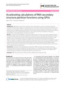
2.1. Tree-based Secondary Structure Representation RNA secondary structure consists of base-paired and unpaired nucleotides. These paired and unpaired nucleotides form a nested structure which can be represented by a rooted tree. In such a tree every base pair corresponds to an inner node while unpaired nucleotides correspond to tree leafs (see Fig. 1). The procedure involves traversing the secondary structure simultaneously from both ends and transforming encountered paired and unpaired nucleotides into inner nodes or leafs of the nascent tree. Fig. 1b shows the result of such transformation.

Fig. 1. (a) Secondary structure of an RNA molecule. (b) Corresponding tree-based representation.

2.2. Tree Edit Distance Algorithm In the following description of the tree edit distance (TED) computation algorithm we follow the notation of [15]. Specifically, by tree we understand a rooted, ordered tree, with 𝑁 symbolizing a set of its nodes and 𝐸 ⊆ 𝑁 × 𝑁 a set of its edges. A forest 𝐹 is an ordered set of trees. Each tree is also a forest. A subforest of a tree 𝑇 is a forest with nodes 𝑁′ and edges 𝐸′ where 𝑁′ ⊆ 𝑁 and 𝐸 ′ ⊆ 𝐸 ∩ 𝑁 ′ × 𝑁′. ∅ denotes an empty tree and 𝑇𝑣 denotes a subtree of 𝑇 rooted in 𝑣, i.e. a tree where only descendants of 𝑣 are preserved. By 𝐹– 𝑣 we understand a forest obtained from 𝐹 by removing node 𝑣 and all edges at v; by 𝐹– 𝐹𝑣 we understand the forest obtained from 𝐹 by removing a subtree 𝐹𝑣 . The tree edit distance metric, a generalization of the well-known string edit distance, is a common similarity measure for rooted ordered trees. Similarly to the string edit distance which is defined as the minimum number of operations needed to convert one structure into another, the tree edit distance represents minimum cost of edit operations (insert, delete, update) that transform one tree into another.

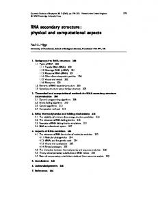
Fig. 2. Illustration of the tree editing operations. The update operations is merely a modification while delete and insert operations require change of the tree topology. The usage of edit operations is illustrated in Fig. 2. While update of a node corresponds simply to its relabeling, the insert and delete operations call for partial remodeling of the tree structure. When deleting a node, its children are reconnected to its parent while maintaining their order. Inserting of a node is

11

Volume 6, Number 1, January 2016

International Journal of Bioscience, Biochemistry and Bioinformatics

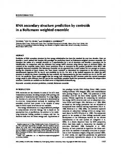
complementary to the delete operation, thus the new node is inserted between an existing node and its children and the children are connected to the newly inserted node. In the heart of TED algorithm is a recursive formula which takes two forests (a tree is a forest of size one) and returns their distance in terms of minimum number of tree edit operations: 𝛿(∅, ∅) = 0 𝛿(𝐹, ∅) = 𝛿(𝐹 − 𝑟𝐹 , ∅) + 𝑐𝑑𝑒𝑙 (𝑟𝐹 ) 𝛿(∅, 𝐺) = 𝛿(∅, 𝐺 − 𝑟𝐺 ) + 𝑐𝑖𝑛𝑠 (𝑟𝐺 ) 𝛿(𝐹 − 𝑟𝐹 , 𝐺) + 𝑐𝑑𝑒𝑙 (𝑟𝐹 ) 𝛿(𝐹, 𝐺 − 𝑟𝐺 ) + 𝑐𝑖𝑛𝑠 (𝑟𝐺 ) 𝛿(𝐹, 𝐺) = min { 𝛿(𝐹 − 𝐹𝑟𝐹 , 𝐺 − 𝐺𝑟𝐺 ) + 𝛿(𝐹𝑟𝐹 − 𝑟𝐹 , 𝐺𝑟𝐺 − 𝑟𝐺 ) + 𝑐𝑢𝑝𝑑 (𝑟𝐹 , 𝑟𝐺 ) In the formula, 𝑟𝐹 and 𝑟𝐺 represent nodes corresponding to roots of trees in forests 𝐹 and 𝐺 , respectively. 𝐶𝑑𝑒𝑙 , 𝐶𝑖𝑛𝑠 , 𝐶𝑢𝑝𝑑 are costs for deleting, inserting or matching nodes. The formula drives a decomposition process which takes two trees and recursively decomposes them into constituting forests for which optimal mapping is then recursively found. The optimal sequence of operations is obtained using dynamic programming. The order in which the roots (𝑟𝐹 , 𝑟𝐺 ) are examined greatly influences the efficiency of the DP algorithm since certain order of roots allows to eliminate some of the subtree calculations. The different approaches are discussed in [16] [15] [17]. As with other dynamic programming-based methods, the steps of the transformation process leading to the minimum distance (tree mapping) can be obtained by backtracking in the dynamic programming matrix. Fig. 3 illustrates the resulting DP matrix using the above formula with 𝐶𝑑𝑒𝑙 = 𝐶𝑖𝑛𝑠 = 1; 𝐶𝑢𝑝𝑑 = 0, the same parameters we use in the experimental section. The rightmost roots were chosen as 𝑟𝐹 and 𝑟𝐺 in each step. Backtracking in this matrix gives us mapping between the two structures, i.e. the sequence of edit operations. In this specific example we can get 𝐺 from 𝐹 by first updating 3 to B, removing node 2 and updating 1 to A.

Fig. 3. Illustration of DP matrix for trees F and G.

2.3. Tree Drawing After we convert the secondary structures of the template and target molecules into tree-based representations and get mapping between the trees using TED, we are ready to use that mapping to convert the template visualization into the target one. We simply follow the backtracking procedure and accompany each tree edit operation with its visual counterpart. In this way, the template is successively turned into target in the order given by the backtracking procedure. Although secondary structure consists of various motifs (see Fig. 4), for the purpose of our visual operations we basically discriminate only stem and loop. Stem is for us any part of the structure which is represented by a sequence of inner nodes in the corresponding tree representation. On the other hand, loop is any part which corresponds to a leaf, no matter whether it is a bulge, interior loop, loop in a hairpin or

12

Volume 6, Number 1, January 2016

International Journal of Bioscience, Biochemistry and Bioinformatics

multibranch loop. Based on whether the tree edit operation involves an inner node (stem) or leaf (loop), we employ two different approaches of how these operations should be reflected in the layout.

Fig. 4. Different motifs of secondary structure. The only operation which does not require significant change in the layout is update. Update of a node corresponds merely to its relabeling. On the other hand, insert and delete operations require to insert or delete a base (leaf) or base pair (inner node) which might affect significant number of other nucleotides in the layout. Here, we describe the visual counterparts for insert and update operations (delete operations are treated the same way, just inversely): 

Inserting leaf. Inserting a leaf into a parent with no leafs corresponds to formation of a new loop. If the parent already contains leafs, then it corresponds to adding a nucleotide into an existing loop. In each case, we simply take all the neighboring leafs and distribute them uniformly on a circle containing the neighboring nucleotides.



Inserting inner node. TED has two ways how to insert a node. In the simpler case, the insert operation involves inserting the new node on a path. In such a case, we insert the corresponding base pair at given position in the layout and then we need to shift all the following paired and unpaired bases. Here we simply use the fact that all affected nucleotides are ancestors of the newly inserted node. Thus, we traverse the affected subtree and shift the nucleotides corresponding to the encountered nodes in given direction. However, TED edit operation can result in insertion of a node accompanied with reconnecting some of leafs from the parent to the newly inserted node. In such a case we basically use multiple operations corresponding to leaf insertions (loop update) and simple inner node insertion (shift). Even though the above described operations are general enough to address almost all situations, multi-branch loops need to be treated individually. When inserting a new branch into multi-branch loop, we need to reorganize all nodes in that loop. Thus, we take all the siblings constituting the multibranch loop and distribute them uniformly on a circle of suitable size. This is similar to the treatment of loops, however this operation requires repositioning (rotating) of all the involved stems.

3. Evaluation We evaluated our algorithm on both synthetic and real data using the state-of-the art secondary visualizations from the CRW database [18] as templates. The same database was also used as the source of the corresponding secondary structures in dot-parenthesis format. In the evaluation, we used pair of structures where we knew the correct layout for both of them and selected one as the template and the other as the target. Then we created a layout for the target using the template and compared it to the known target visualization. The evaluation was subject to visual inspection (see examples below) and automatic evaluation of planarity of the layouts expressed as the number of crossing base pairs.

13

Volume 6, Number 1, January 2016

International Journal of Bioscience, Biochemistry and Bioinformatics

To see how insert and update operations work, we extracted a simple hairpin and multibranch loop from the human 16s rRNA and showed how insertion and/or removal of selected bases changes the layout. In all the images we use the following color convention: black letters represent non-loop bases that have not been changed, i.e. the same nucleotides in the same position in template and target layout; blue letters represent loop nucleotides which were present in both template and target but had to be repositioned in the target; red letters represent inserted bases, i.e. those which were present in target but not in the template; green letters represent bases which were relabeled, i.e. they occupy the same position in the template and target but the letter differs.

Fig. 5. Example of insertion (red bases labeled as I) into a hairpin. Fig. 5 shows the effect of adding several bases into a hairpin. We simulated inserts into both stem and loop parts of the hairpin. We can see that inserting four nucleotides into loop requires its redrawing so that all the bases forming the loop are evenly distributed on a circle. Second insert involves insert on both sides of a stem. One strand received a new base while the other received 5 new bases forming a new bulge. A little bit more complex example illustrates Figure 6 where we show the effect of substantial deletion of one branch of a multibranch loop (Fig. 6a). We focused on the upper branch and removed all the base pairs after the interior loop. Such operation resulted into degradation of the interior loop into a simple loop as illustrated by Fig. 6b. Then we took the modified structure and used it as a template for the original multibranch loop structure, i.e. we reinserted the removed nucleotides (for better orientation we labeled them “I” in the visualization). Fig. 6c shows that we were able to rebuild the original layout with only minor changes in positions of the nucleotides (for example the blue loop at the end of the stem is slightly denser).

Fig. 6. Delete (b) and reinsertion (c) of the deleted bases into a stem of a multibranch loop (a). Next, we tested the ability of our algorithm to reconstruct visualizations of known 16S ribosomal subunits from the Metazoa kingdom. The CRW database contains structures of 16 organism with existing dot-bracketing information: Androctonus australis, Artemia salina, Drosophila melanogaster, Echinococcus granulosus, Homo sapiens, Microciona prolifera, Mnemiopsis leidyi, Mus musculus, Mytilus edulis,

14

Volume 6, Number 1, January 2016

International Journal of Bioscience, Biochemistry and Bioinformatics

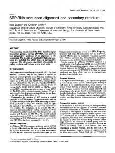
Okanagana utahensis, Oryctolagus cuniculus, Placopecten magellanicus, Rattus norvegicus, Tripedalia cystophora, Xenopus borealis, Xenopus laevist . Ribosomal RNA structures were chosen because they are in the research focus of many biological users and because their length and complexity makes them particularly challenging for visualization methods. We ran the visualization algorithm for every pair of structures resulting in 256 layouts. We experiences only minor problems which was reflected in 3 crossings per layout on average, i.e. 3 violations of planarity in the resulting layouts. The resulting layouts can be downloaded at http://siret.cz/rnavisds. Fig. 7 shows an example of visualization of Human rRNA using Artemia salina (shrimp) as a template. Although the organisms are relatively far apart, our algorithm was able to reconstruct the layout with only one error.

Fig. 7. Reconstruction of Human 16S rRNA using Artemia salina (shrimp) as a template. The black circle in upper left part shows the only error.

4. Discussion The proposed method is based on the same principle as, for example, homology-based modelling. That brings one problem; when the template layout contains some specific features which are not accounted for in the algorithm their visualization might go awry. For example, rRNA visualization in the CRW database use specific layout for long unpaired bases (not resolved parts of the structure) which we cannot mimic since there is no good definition for them. Another issue is the inability of the method to correctly draw a structure for which no close homologue exists. For example, if the target contains a hairpin which includes another hairpin and these are not present in the template, our algorithm will not output a good layout. This problem probably could be approached using recursive layout procedure. Finally, in its current version, our algorithm does not handle pseudoknots in any way.

15

Volume 6, Number 1, January 2016

International Journal of Bioscience, Biochemistry and Bioinformatics

5. Conclusion We have introduced a new method for drawing RNA secondary structures using a template visualization. Such an approach tackles the lack of standards or formal requirements in the field of secondary structure visualization. The algorithm is able to produce high-quality visualizations in case a sufficiently similar structure with an existing visualization exists. Such a situation arises, for example, in case of ribosomal RNAs which exhibit a well conserved regions with smaller, less conserved parts. In the future we would like to extend the method to situations when the template substantially differs from the target layout.

Acknowledgment This work has been supported by the Czech Science Foundation grant 15-00885S and by Charles University projects P46 and SVV-2015-260222. The access to computing and storage facilities owned by parties and projects contributing to the National Grid Infrastructure MetaCentrum, provided under the programme ”Projects of Large Infrastructure for Research, Development, and Innovations” (LM2010005) is highly appreciated.

References [1] Puton, T., et al. (2013). CompaRNA: A server for continuous benchmarking of automated methods for RNA secondary structure prediction. Nucleic Acids Res, 41(7), 4307-4323. [2] Pánek, J., Hajic, J., & Hoksza, D. (2014). Template-based prediction of ribosomal RNA secondary structure. IEEE International Conference on Bioinformatics & Biomedicine (pp. 18-20). [3] Tamassia, R. (2007). Handbook of Graph Drawing and Visualization (Discrete Mathematics and Its Applications). [4] Scott, J. (1988). Social Network Analysis. Sociology-the Journal of the British Sociological Association, 22(1), 109-127. [5] Wiese, K. C., Glen, E., & Vasudevan, A. (2005). JViz.Rna—a Java tool for RNA secondary structure visualization. IEEE Trans Nanobioscience, 4(3), 212-218. [6] Lorenz, R., et al. (2011). ViennaRNA Package 2.0. Algorithms Mol. Biol., 6, 26. [7] Darty, K., Denise, A., & Ponty, Y. (2009). VARNA: Interactive drawing and editing of the RNA secondary structure. Bioinformatics, 25(15), 1974-1975. [8] De Rijk, P., Wuyts, J., & De Wachter, R. (2003). RnaViz 2: An improved representation of RNA secondary structure. Bioinformatics, 19(2), 299-300. [9] Zuker, M. (2003). Mfold web server for nucleic acid folding and hybridization prediction. Nucleic Acids Res, 31(13), 3406-3415. [10] Han, K., Lee, Y., & Kim, W. (2002). PseudoViewer: Automatic visualization of RNA pseudoknots. Bioinformatics, 18(Suppl 1), 321-328. [11] Byun, Y., & Han, K. (2006). PseudoViewer: Web application and web service for visualizing RNA pseudoknots and secondary structures. Nucleic Acids Res, 34(Web Server issue), 416-422. [12] Byun, Y., & Han, K. (2009). PseudoViewer3: generating planar drawings of large-scale RNA structures with pseudoknots. Bioinformatics, 25(11), 1435-1437. [13] Yang, H., et al. (2003). Tools for the automatic identification and classification of RNA base pairs. Nucleic Acids Res, 31(13), 3450-3460. [14] Auber, D., et al. (2006). Efficient drawing of RNA secondary structure. J. Graph Algorithms Appl., 10(2), 329-351. [15] Zhang, K., & Shasha, D. (1989). Simple fast algorithms for the editing distance between trees and related problems. SIAM J. Comput., 18(6), 1245-1262.

16

Volume 6, Number 1, January 2016

International Journal of Bioscience, Biochemistry and Bioinformatics

[16] Demaine, E. D., et al. (2009). An optimal decomposition algorithm for tree edit distance. Acm Transactions on Algorithms, 6(1). [17] Pawlik, M., & Augsten, N. (2011). RTED: A robust algorithm for the tree edit distance. Proc. VLDB Endow, 5(4), 334-345. [18] Cannone, J. J., et al. (2002). The comparative RNA web (CRW) site: An online database of comparative sequence and structure information for ribosomal, intron, and other RNAs. BMC Bioinformatics, 3, 2.

Richard Eliáš is pursuing his bachelor degree at department of software engineering at faculty of Mathematics and Physics, Charles University in Prague. His research focuses on the graph algorithms and their application in bioinformatics.

David Hoksza received the PhD degree from the department of Software Engineering, Charles University in Prague, Prague, Czech Republic, in 2010. Since 2011, he has been an associate professor of software engineering in the department of Software Engineering at the Charles University in Prague and among years 2011 and 2015 he was an assistant professor in the laboratory of Informatics and Chemistry at the Institute of Chemical Technology, Prague. His current research interests include structural bioinformatics, chemical informatics, data engineering and similarity searching.

17

Volume 6, Number 1, January 2016