We presented a novel procedure to extract ground road networks from airborne LiDAR data. First point clouds were separated into ground and non-ground parts ...
Road Network Extraction from Airborne LiDAR Data using Scene Context Jiaping Zhao Suya You University of Southern California Los Angeles, CA 90089 {jiapingz,suya}@usc.edu
networks, aiming to detect roads with different reflective spectra, varied widths and orientations, overlapped mutually, and even occluded by trees partially or globally. Our contribution is manifold: (1) proposed two novel features, flatness and convexity, to discriminate buildings and trees; (2) designed structure templates to fit local road shapes, and presented a voting scheme to determine road widths and orientations; (3) constructed a Markov graph, which explicitly incorporates scene knowledge, to make a global inference on road networks.
Abstract We presented a novel procedure to extract ground road networks from airborne LiDAR data. First point clouds were separated into ground and non-ground parts, and ground roads were to be extracted from ground planes. Then, buildings and trees were distinguished in an energy minimization framework after incorporation of two new features. The separation provided supportive information for later road extractions. After that, we designed structure templates to search for roads on ground intensity images, and road widths and orientations were determined by a subsequent voting scheme. This local searching process produced road candidates only, in order to prune false positives and infer undetected roads, a scene-dependent Markov network was constructed to help infer a global road network. Combination of local template fitting and global MRF inference made extracted ground roads more accurate and complete. Finally, we extended developed methods to elevated roads extraction from non-ground points and combined them with the ground road network to formulate a whole network.
2. Related Work We briefly review works on road extraction from spectral imageries and LiDAR data. In [6], the authors made use of both height and intensity information to hierarchically classify point clouds into roads and non-roads. Hu et al.[7] relied mainly on LiDAR data, with some support from aerial images, to extract urban grid networks. They developed an iterative Hough Transform procedure to detect straight ribbons and used a hypothesis-test scheme to do verification. Zhu and Mordohai[1] addressed road network extraction from LiDAR by first performing segmentation using boundary and interior features on intensity images and then employing minimum cover set algorithm to search the most possible set of segments. Volodymyr et al.[5] presented a neural network learning approach to detect roads on high-resolution aerial images. The proposed neural network contains millions of trainable weights which take a large context into account. In [4], Pechaud et al. extracted tubular structures on 2D images by searching shortest geodesic paths in a 4D space. For works focusing on road networks, Ting et al. [3] presented phase field higher-order active contour models, and exploited them to segment road network from high resolution images. Tupin et al.[8] first detected individual line segments from SAR images, and then modeled interactions among line segments by MRF and network extraction was transformed into a MRF labeling problem. Negri et al.[13] integrated road junction information into the road network extraction process and made an improvement over the approach using no junction information when experimenting on SAR images. In [12],
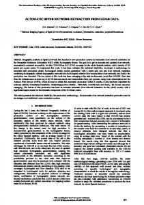
1. Introduction Network extraction has a wide application in remote sensing, medical imaging and computer vision. For road network extraction, different methods have been suggested under different situations, some dealing with roads on satellite and aerial images while others working on LiDAR data. In this article, we focus on ribbon-road network extraction from airborne LiDAR data. On 2D imageries, fully automatic and high-accuracy road extraction is still challenging due to occlusion by trees (Fig.1(a)), self-overlapping (Fig.1(b)), disturbance of similar reflective objects and lack of context knowledge. There are several solutions like incorporating external geographic information [2], making assumptions on road intensity distributions or taking advantage of prior constraints on the geometry of networks[9]. Compared to 2D imageries, airborne LiDAR data provides additional 3D coordinates. This geometric information may help us to handle those tricky cases in 2D. In this paper, we rely solely on LiDAR data with no external information to extract road
1
(a) Atlanta (b) Oakland Figure 1. Advantages of LiDAR data for road extraction. There are two datasets, (a) from Atlanta and (b) from Oakland. The left shows original point clouds, and the right is extracted roads. In the Atlanta region, roads are heavily occluded by trees, making traditional 2D-based methods hard to work, however, occluded roads are correctly inferred by our method (blue points). In case two, it shows highly overlapped viaducts, which are difficult to be traced on 2D images. By making additional information provided by LiDAR, they are correctly separated and extracted. Extracted roads are superimposed on the satellite image.
authors modeled the line network by an object process. Their model considered both topological and radiometric properties of line networks, and was optimized by RJMCMC algorithm. In our work, we aim to extract both ground and elevated roads from airborne LiDAR data, and formulate them into a connected road network.
4. Ground and non-ground separation Elevated roads will be self-overlapping, and every individual one will have a different elevation. However, roads on ground have the same height locally and won’t be overlapped. Due to different characteristics, they will be extracted in separate procedures. So we separate point clouds into ground and non-ground first: the former for ground roads extraction and the latter for elevated roads extraction. Point clouds are first converted into 2D depth images, and separation is implemented on them. Morphological filtering is a major kind of methods for digital terrain model ( ) generation [16] from depth images. Opening is a successive operation of erosion and dilation, after which elevated objects smaller than the structure element ( ) are removed while terrain is retained. However, the larger the is, the less accurate the reconstructed terrain is. To address this problem, several scholars [6,16] proposed hierarchical strategy: first using large SE to remove large objects, and decreasing its size gradually to remove small objects like vehicles and individual trees. We adapt the hierarchy strategy in [6] to separate grounds from elevated objects. The output of the hierarchy strategy is a , and by subtracting from depth images, pixels where absolute difference values are greater than certain threshold are elevated, otherwise they are on the ground.
3. Overview of the approach We start by separating non-ground points from ground planes by hierarchical morphological opening. Then we classify elevated points into two classes: buildings and trees. With a slight abuse of terminology, in the rest of the paper, we call all elevated man-made objects as buildings. Two features, flatness and convexity, are presented to discriminate them. Their separation helps to support the later ground road extraction. Moreover, elevated roads are to be extracted from buildings. Afterwards, we search ground road candidates from the ground plane. To get road widths and orientations simultaneously, elongated structure templates with varied widths and directions are designed to fit local intensity distributions and a subsequent field voting scheme is introduced to refine candidate widths and orientations. Then, we model interactions among ground road candidates through a Markov graph, formulating ground road network extraction as a labeling problem. Finally, we extended the developed method to extract elevated roads. The combination of extracted ground and elevated roads are final outputs. The pipeline of road network extraction system is shown in Fig. 2.
5. Buildings and trees separation Buildings and trees have distinct spatial relationships with roads, concretely, projection of buildings onto plane won’t overlap with roads, while this is not true for trees, e.g. in case where roads are occluded by trees. In later road extraction steps, we will use this scene knowledge to construct road networks. As a preparation step, elevated points are partitioned into buildings and trees. Two features, flatness and convexity, are devised to distinguish them. After initial binary labeling
Figure 2. Pipeline of road extraction system
2
1. For each facet "# with vetices { , , ! }, the other 6 points are partitioned into two groups according to their distances to "# : one group having positive distances and the other having negative ones. Supposing the maximum absolute distance in each group is $ %& and $'() respectively, we assign value *+ ( $ %& , $'() ) to facet "# , i.e. let $,- = *+ ( $ %& , $'() ). 2. Each facet gets its assigned value $,- and convexity at point is defined as */0 ($,1 , $,2 , ⋯ , $,3 ).
(0 for trees and 1 for buildings) of elevated pixels based on two feature values, we solve their optimal labels in an energy minimization framework.
5.1. Flatness Definition 1 (Flatness): For a pixel on 2D depth image, its neighbors are pixels covered by a × window centering on . Flatness at pixel is defined by votes gotten by after a voting process: for a neighboring pixel ( ∈ , ≠ ), if the included angle between its normal and (normal at ) is smaller than threshold , then it will vote . After all − 1 neighbors finish voting, votes accumulated by is defined to be flatness at , and this voting process is called cumulative voting. The larger the number of votes one point gets, the flatter it is locally at that point. Ideally, if all normals have the same direction, flatness at is − 1 ; to another extreme, assuming normal distributes randomly, and the included angle between any pair of normals is greater than , then flatness at is 0. Generally, normal distribution over a tree crown is random, while its distribution on a local roof, especially a planar roof, has one dominant direction. Flatness is illustrated in Fig.3.
For points lying on locally convex surfaces (sphere, cone and cylinder shaped roofs), their convexity values are 0, while for tree canopy surfaces, they are no more locally convex, so points on them have larger convexity values.
Figure 4. Convexity. (a) Left: the surface going through the central point is locally convex, so convexity at the central point is 0. Right: a non-convex surface through the central point, convexity at the central point is a positive value; (b) Convexity computation at pixel v0 on depth images
5.3. Segmentation by energy minimization After computation of flatness and convexity for elevated pixels, we use MRF to classify them into building and trees. Only first and second order potentials are considered and 8-neighborhood is used as the neighboring norm. The pairwise interaction is defined by the standard Potts model [10] and the data term is a combination of two features defined above:
Figure 3. Flatness. Left: on a locally planar surface, normals have similar directions, and cumulative voting produces a high value; Right: on an irregular surface, normal directions are randomly distributed, and cumulative voting produces a low value.
5.2. Convexity
45
Cumulative voting is especially effective for identifying planar roofs. However, for sphere, cone, cylinder and other shaped roofs, it’s less distinctive, because normal still varies within a local region. In order to avoid misclassifying these kinds of roofs as trees, we propose convexity. The intuition behind convexity is that most roof surfaces are locally convex, which is usually not true for tree crown surfaces. Definition 2 (convexity at a point): on 2D depth images, we quantize local convexity of surface at pixel using a numerical value. As in Fig. 4(b), { , , ⋯ , } are 8-neighboring pixels of . Any two consecutive neighbors { , ! } , together with , form a triangular facet "# . There are totally 8 facets {" , " , ⋯ , " } , which are the on surface . The convexity of facets going through surface at pixel is calculated as follows:
,5 85
=
,5
+7
: ;,5
85
= 9 , ;('2 ; ) : 5 /C 1−C / =A 1 − /C C/
+" + ∈ ?
+" + +" C +" C +" C +" C
∈ @::? (1) ≤ ∩ + ∈ @::? > ∩ + ∈ @::? > ∩ + ∈ ? ≤ ∩ + ∈ ?
Where " and cH are flatness and convexity at pixel i and n is the size of the cumulative voting window. A graph-cut algorithm [10] is used to solve this optimization problem. It’s easy to check that our model fits the requirements of this algorithm. There are three parameters, namely and 7, K. Parameters 7 balance energy within data term, while K adjusts ratio between data and interaction terms. In the experiment, we set = 0.3, 7 = 0.5, K = 0.5. Although
3
width
rigorously one should learn them through labeled samples, we notices that this parameter setting performs well on a variety of LiDAR datasets.
6. Ground road candidates extraction Ground roads are contained on the ground plane. Since neighboring points on ground have similar elevations, elevation is not a good cue for identifying roads from other ground objects such as parking lots and grass land. Therefore, we disregard depth information and search roads on 2D intensity maps of ground points. This section presents template fitting and field voting methods to extract road candidates.
Figure 5. Fitting template: (a) template; (b) shifting center within region R ; (c) designed templates of different widths and orientations
6.1.2 Road saliency within template area Given a template , how to measure the probability of existence of a road with the same orientation and width within the template area? When observed locally from an image, roads are perceptible especially when their intensity deviates from that of the background. Here we use fisher discriminant to capture the local dis-similarity of intensity distribution between road and background, which takes the form
6.1. Template fitting to search roads Roads on aerial LiDAR data are ribbon-shaped elongated regions instead of one-pixel width curves. In order to extract roads of various widths and orientations, we devised elongated structure templates with varied sizes and directions. Search of road parameters is equivalent to template fitting.
?=
A typical elongated structure template with width w and height h is shown in Fig. 5(a), and it captures the local geometry of a vertical road with width w. This template has three contiguous parts R , R , RS , in which R indicates roads and R , RS indicates non-roads. R , RS are both half of the width of R . A standard template of size U × ℎ is defined as (1: road regions, 0: non-road regions):
We allow template center shiftable within R , Fig.5(b) shows a center-shiftable template. By not centering the template on the point under consideration, we can find a shift that best fits it with local roads. Given a point p on roads, to compute its road saliency ? under template , we compute fisher discriminants for all shifts and keep the maximum saliency as the saliency under template . Compared to center-fixed templates, there are obvious merits: the saliency produced for a point near road sides are at the same level as that produced for a point at the road center. Suppose is the template producing the maximum saliency at p, and is called fitting template and its width and orientation is said to be the candidate width and orientation of the road going through .
Two parameters (@, \) are introduced to generate templates with varied widths and orientations from the standard template : ^
_`
∙
(4)
6.1.3 Template fitting
0 < 0 < 0.5 ∙ U , 0 < W < ℎ 0.5 ∙ U < 0 < 1.5 ∙ U , 0 < W < ℎ (2) 1.5 ∙ U < 0 < 2 ∙ U , 0 < W < ℎ (@, \) = R] ∙
2 &h2 !&ih
Where *^ , *'^ are respectively the mean intensity values within R and R ∪ RS , and ?^ , ?'^ are the corresponding standard variances. The value of fisher discriminant ? is called road saliency here.
6.1.1 Local structure templates
0 (0, W) = X1 0
(ch ;cih )2
(3)
Where R] is the planar rotation matrix of angle \, and @ is the designated template width. Each template (@, \) represents a road oriented along direction \ with width @. Direction \ lies within [0, b) , and @ ∈ [Uc ' , Ucde ] , where Uc ' , Ucde are respectively widths of narrowest and widest roads in the scene. Scaled and rotated templates are shown in Fig. 5(c). The choice of ratio g = ℎ/U between height and width of templates is a trade-off between robustness and accuracy of local road detectors. The larger the ratio is, the more robust the detector is, while the smaller the ratio is, the more accurately the detector performs. In the experiment, we let g = 2.5.
6.2. Field voting to determine road widths and orientations Candidate width and orientation at each point are not necessary the true width and orientation of the road going through that point. To get road width and orientation as close as possible to the true ones, we designed a voting scheme, during which width and orientation information are propagated into neighborhood. After determination of fitting template at , a voting
4
field lm is created as follows: (1) lm is a rectangle, having the same width and orientation as ; (2) lm is fitted to lie between R and RS and overlaps with R of ; (3) p lies on the center line of voting field lm . The extension of lm along the road candidate direction is V lm , i.e. points as far as V lm /2 apart from p along that direction will still be covered by lm . The ratio gn . V lm /U lm is set by making a balance between accuracy of road detection and gap filling capability of voting field. Fig.6 shows a fitting template and the constructed voting field. Each point on the ground mask maintains an accumulator array, with one dimension referring to quantized widths U U ∈ aUc ' , Ucde f and the other to quantized orientations \ \ ∈ a0, b . When it falls within a voting field lm , it gets one vote and its accumulator array at position U lm , \ lm increases by one. After it collects votes from all neighboring fields, the position of the peak value in its accumulator array is the width and orientation of roads going through it. In the experiment, a point with the peaking votes less than ogn U ( o Y 1, U is the road width at ) will be removed. All left points consist of road candidates.
7.1. Centerline tracking For the convenience of management, centerlines of road candidates are tracked and used to substitute for road ribbons. We introduce a multi-step marching algorithm. This algorithm makes a balance between simplicity and accuracy: for a straight road, marching steps are large and it’s finally represented by few long line segments, while for a curvy road, marching steps are adjusted adaptively to shorter ones, making the representation more accurate. This algorithm works on votes maps, and finds the point with the maximum votes as the start marching point. Marching begins along the road direction at current point, and a larger marching step is used first, if the difference between road direction at the next potential point and current marching direction is less than certain value, that point is accepted and marching continues from that point. Otherwise, a smaller step is used until the next valid point is found or road ends have been reached. This process iterates until no road candidates are left.
Figure 8. Centerline tracking. Left: starting from p , a larger step M is used first, but because of a large direction difference between p€ and p , p€ is an invalid next point; decease the marching step, and find a valid point p . Right: tracked center
lines. Figure 6. Constructing voting field according to fitting template
7.2. Missing roads hypothesis First we make hypotheses on potential missing roads based on network geometry and scene knowledge.
7. Ground road network construction Field voting propagates road widths and orientations into neighborhoods, therefore effects of local tree occlusions are compensated (Fig. 7). However, for roads largely occluded by trees, they can’t be detected. In this section, we model road networks as a Markov graph, in order to infer undetected roads and prune false road candidates.
7.2.1 Road network geometry Wholly based on geometry of tracked centerlines, missing roads happen in two cases most often: (1) gaps between segments (Fig. 9); (2) T-intersection connection (connection between one end point and a potential T-intersection). We use criteria in [14] to measure the possibility of every gap connection, and keep top possible gap connections. For a potential T-intersection connection, the possibility of its existence is measured by: pq . sin \ ∙ s1 6 exp v
wxy
;
{|
Where, \ is the included angle between reference and target segment, and right angle is preferred. )d and }d^ are lengths of gap and target segment respectively (Fig.9). Top m possible T-intersection connections are kept.
Figure 7. Compensation of local tree occlusion by field fitting. Left: intensity image; right: votes map. The brighter it is, the more votes it gets. We can see from the votes map that occluded areas will also get votes.
5
zxh
(5)
roads in open areas are much less possible to be undetected due to the completeness for road candidate extraction. When there is a large portion of trees in the hypothesized missing ribbons, possibility of being a road is pushed up rapidly. For interaction terms, two different connections are modeled separately. Gap intersection is modeled by a standard Potts model, which favors smoothness. For T-intersection connections or intersecting relations, the penalty is given by:
Figure 9. Two types of potential connections for missing road hypotheses
7.2.2 Context knowledge to filter hypothesized missing roads
•ŽH• 5 , ‘ cos \ ‹Ž“” , 5 ‘ „… . sin \ Ž“” • Œ ‹ ŽH• 5 , ‘ sin \ Š ŽH• •
For m + n proposed missing roads, if any one going across a building, then it is rejected and removed from initial hypotheses. Left ones are kept as missing road candidates.
Ž“” •
Based on the observation that roads are generally connected, interactions among segments are modeled by a graph. A node corresponds to either a road candidate or a missing road candidate, and an edge exists between two nodes if they are gap-connected, T-intersection connected or intersecting each other. Road network extraction is equivalent to the labeling of segments in the graph. This labeling procedure is performed under the MRF framework with unary and pairwise potentials. The quality of the labeling is measure by the energy: 6K∑
,… †‡ „ …
, , $ƒ
5
+" $ +" $ +" $ +" $
0.5$ /$ c .A c 0.5$ /$
D$ F$ F$ D$
∩ ∩ ∩ ∩
.1 .1 .0 .0
5
.9
!( h
C
.1 .0
.0
(9)
…
Figure 10. MRF missing roads inference. Left: intensity image. As we see, roads are largely occluded by trees. Middle: gray segments are road candidates after template fitting and field voting; green ones are inferred missing roads. You can notice that there are two kinds of missing roads-gap connection and T-connection; Right: inferred road networks by MRF.
(7)
8. Elevated road extraction
Where $ is the length of + segment, and C , C ∈ a0,1f with C Y C . For hypothesized ones, penalty is defined in terms of a ratio between areas of trees and ground within the hypothesized ribbon: }ˆ
…
.1
(6)
Where + corresponds to a tracked centerline or a hypothesized one, is the label of + (1 for true roads and 0 otherwise), and „ … are data and interaction terms, balanced by a parameter K. In the model, interaction term „ … is data dependent on segment lengths $ƒ . Different data terms are used for tracked roads and hypothesized ones. For tracked roads, penalty is defined in terms of length: 1
.
…
Where \ is the T-connection or intersecting angle. Find the labeling configurations, which minimizing the penalty • is a non-convex optimization problem. However, in a 1–* scene, there are generally 200~300 segments, optimization using standard iterated conditional mode approach, graph cut[10] and Gibbs sampling method can be very fast to get an approximately global optimal solution. In the experiment, graph-cut algorithm takes 2s for 200 segments. Ground road network extraction results from a heavily occluded area are shown in Fig. 10.
7.3. Road network formulation
• . ∑ ∈ƒ
.
Until now, designed methods are oriented to extract roads on the ground, precluding all elevated roads. However, template fitting, filed voting and marching algorithms are easily extended for elevated roads extraction from buildings. There are two major differences: We use template correlation, instead of Fisher discriminant, to compute local road saliency. The normalized cross-correlation value between reference template ^ and target template ) is used as road saliency. ^ has value 1 in region R and 0 in R ∪ RS , while values in ) are determined as follows: for an elevated pixel under consideration, let ^ , '^ be its neighboring pixels in
(8)
Where C ∈ a0,1f and penalizes non-roads. A sigmoid function is used to penalize . 1 @‰/$ due to the fact that missing roads are generally occluded by trees, while
6
Figure 12. Building separation from trees using flatness and convexity. Top Left: point clouds; Top Right: flatness map; Bottom Left: convexity map; Bottom Right: detected buildings
Figure 13. Local template fitting and field voting to extract roads under varying conditions. Left: LiDAR point cloud; Right: extracted road networks superimposed on intensity images; the 1st row: various intensity scopes; the 2nd row: curvy roads; the 3rd row: several widths; the 4th row: local tree occlusion
Table 1. Evaluation of road extraction results
Denver Atlanta
True length(–*) 269.4 421
True positives(–*) 247.4 367.1
False positives(–*) 30 48.2
completeness
correctness
quality
91.8% 87.2%
89.2% 88.4%
82.6% 78.3%
[4] Mickael Pechaud, Renaud Keriven, Gabriel Peyre. Extraction of Tubular Structures over an Orientation Domain. CVPR, 2009 [5] Volodymyr Mnih and Geoffrey E. Hinton. Learning to detect roads in high-resolution aerial images. ECCV, 2010 [6] Simon Clode, Peter Kootsookos, Franz Rottensteiner. The automatic extraction of roads from LiDAR data. ISPRS. [7] Hu, X., Tao, C.V. and Hu, Y. Automatic Road Extraction From Dense Urban Area by Integrated Processing of High Resolution Imagery and LiDAR Data. In IAPRSIS, 2004 [8] F. Tupin, H. Maitre, J. F. Mangin, J. M. Nicolas and E. Pechersky. Detection of linear features in SAR images: Application to road network extraction. IEEE Trans. Geosci. Remote Sensing, vol. 36, pp. 434-453, 1998 [9] B.K. Jeon, J.H. Jang and K.S. Hong. Road detection in spaceborne SAR images using a genetic algorithm. IEEE Trans. Geosci. Remote Sens., 40(1), pp. 22-29, 2002 [10] Y. Boykov, O. Veksler, and R. Zabih. Fast Approximate Energy Minimization via Graph Cuts. IEEE Trans. PAMI, 23(11), pp. 1222-1239, 2001 [11] I. Laptev, H. Mayer, T. Lindeberg, W. Eckstein, C. Steger, and A. Baumgartner. Automatic extraction of roads from aerial images based on scale space and snakes. Machine Vision and Applications, 12(1):23–31, 2000 [12] C. Lacoste, X. Descombes and J. Zerubia. Point processes for unsupervised line network extraction in remote sensing. IEEE Transactions on Pattern Analysis and Machine Intelligence, 27(10), pp. 1568-1579, 2005 [13] M. Negri, P. Gamba, G. Lisini and F. Tupin. Junction-aware extraction and regularization of urban road networks in high-resolution SAR images. IEEE Trans. Geosci. Remote Sens., 44(10), pp. 2962-2971, 2006 [14] J. Zhao, S. You, J. Huang. Rapid Extraction and Updating of Road Network from Airborne LiDAR Data. in AIPR, 2011 [15] Hu, J.. Road Network Extraction and Intersection Detection From Aerial Images by Tracking Road Footprints. IEEE Transactions on Geoscience and Remote Sensing, 2007 [16] K. Zhang, S-C. Chen, D. Whitman, M-L. Shyu, J. Yan and C. Zhang. A progressive morphological filter for removing non-ground measurements from airborne LiDAR data. IEEE IEEE Trans. Geosci. Remote Sensing, 2003
9.3. Road network extraction evaluation We have experimented on two datasets: Denver and Atlanta areas. Denver dataset covers 20 –* downtown areas, most of objects are buildings and there are only few trees, while Atlanta data covers 35 –* downtown and residential regions, where many roads are occluded by trees. The extracted roads were compared with ground truth roads, which were manually labeled on intensity images, using aerial images for verification. Only centerlines were labeled. Then three indexes [15] (1) completeness (2) correctness and (3) quality are used to evaluate the extraction results. Although our algorithm extracted both road centerlines and boundaries, we only compared centerlines with labeled roads. If the labeled roads are falling within the extracted road ribbons, then the corresponding road centerlines are true positives. If no labeled roads fall within an extracted ribbon, then the corresponding centerline is a false positive. When a labeled road isn’t covered by any extracted ribbons, then it is an undetected road. Statistics for two datasets show in table 1. In Denver areas, there is much less occlusion, and most roads are extracted during template fitting and field voting, however, in more occluded Atlanta areas, although road candidates are incomplete, many undetected roads are inferred by later scene-context embedded Markov network.
10. Conclusions In this paper, we proposed an original procedure for road extraction from aerial LiDAR Data. The main strength of the procedure is that it combines a robust local detector with a global context-incorporating graph to reach both high correctness and completeness. However, for occluded curvy roads, there is less probability to be detected by our graph model. Moreover, elevated and ground roads are extracted in separate processes, so their interactions are not yet considered. These problems are our further work.
References [1] Qihui Zhu, Philippos Mordohai. A Minimum Cover Approach for Extracting the Road Network from Airborne LiDAR data. ICCV workshop, 2009 [2] Aleksey Boyko, Thomas Funkhouser. Extracting roads from dense point clouds in large scale urban environment. ISPRS [3] Ting Peng, Ian H. Jermyn, Veronique Prinet, Josiane Zerubia. Extended phase field higher-order active contour models for networks. IJCV, 2010
8