Road profile estimation using neural network algorithm - Springer Link

Journal of Mechanical Science and Technology 24 (3) (2010) 743~754 www.springerlink.com/content/1738-494x

DOI 10.1007/s12206-010-0113-1

Road profile estimation using neural network algorithm† Mahdi Yousefzadeh, Shahram Azadi* and Abbas Soltani Department of Mechanical Engineering, K. N. Toosi University, Tehran, Iran (Manuscript Received January 22, 2009; Revised September 20, 2009; Accepted November 8, 2009) ----------------------------------------------------------------------------------------------------------------------------------------------------------------------------------------------------------------------------------------------------------------------------------------------

Abstract This paper more specifically focuses on the estimation of a road profile (i.e., along the "wheel track"). Road profile measurements have been performed to evaluate the ride quality of a newly constructed pavement, to monitor the condition of road networks in road management systems, as an input to vehicle dynamic systems, etc. The measurement may be conducted by a slow-moving apparatus directly measuring the elevation of the road or using a means that measures surface roughness at highway speeds by means of accelerometers coupled with high speed distance sensors, such as laser sensors or using a vehicle equipped with a response-type road roughness measuring system that indirectly indicate the user's feelings of the ride quality. This paper proposes a solution to the road profile estimation using an artificial neural network (ANN) approach. The method incorporates an ANN which is trained using the data obtained from a validated vehicle model in the ADAMS software to approximate road profiles via the accelerations picked up from the vehicle. The study investigates the estimation capability of neural networks through comparison between some estimated and real road profiles in the form of actual road roughness and power spectral density. Keywords: Road profile; Simulation; Artificial neural network; Power spectral density; Estimation ----------------------------------------------------------------------------------------------------------------------------------------------------------------------------------------------------------------------------------------------------------------------------------------------

1. Introduction Road profile is one of the most effective vehicle environmental conditions that influences ride, handling, fatigue, fuel consumption, tire wear, maintenance costs, vehicle delay costs, etc. Therefore, establishment of methods for road profile measurement is completely essential. Currently, many routines are available for road profile measurement. Most of them measure vertical deviations of the road surface along the traveling wheel path. The American Society of Testing and Materials (ASTM) standard E867 defines road roughness as the deviations of a pavement surface from a true planar surface with characteristic dimensions that affect vehicle dynamics, ride quality, dynamic loads, and drainage [1]. First attempts for road profile measurements started around the 1920s with a straight edge device. Since then, traditional profilers have evolved to vehicles that can measure the road profile while traveling at a normal traffic speed. These equipments measure longitudinal profiles, which provide vertical elevation as a function of longitudinal distance along a prescribed path. Generally, these equipments can be divided into the following five categories [2]:

1.1 Response-type road roughness measuring systems (RTRRMSs) RTRRMS measures the response of a vehicle to the road profile using transducers to accumulate the vertical movement of the axle of the trailer (Fig. 1) or the vehicle (Fig. 2) with respect to the vehicle frame. The measurement directly reflects the user's feelings of the ride quality. These devices have the disadvantage of the measured results being influenced by the properties of the vehicle mechanical system and measuring speed.

Fig. 1. Schematic diagram of a BPR roughometer from the Bureau of Public Roads [1].

†

This paper was recommended for publication in revised form by Associate Editor Kyongsu Yi * Corresponding author. Tel.: +98 21 8867 4841, Fax.: +98 21 8867 4748 E-mail address: [email protected] © KSME & Springer 2010

Fig. 2. An RTRRMS schematic of Mays ride meter [2].

744

M. Yousefzadeh et al. / Journal of Mechanical Science and Technology 24 (3) (2010) 743~754

Fig. 4. California-type profilograph, model ES2000 [4].

Fig. 3. Dynatest road surface profilometer, model 5051 MK II L3.2cg, used in Bulgaria [3].

1.2 High speed inertial profilers

Fig. 5. California-type profilograph [4].

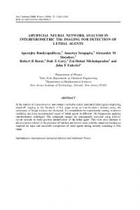
The first inertial profiler was developed in 1960 by Spangler and Kelly at the General Motors Research Laboratories. These types of profilers collect pavement profile data at highway speeds and generate the true profile of a roadway, which is shown in Fig. 3. The main components of an inertial profiler are their height sensors, accelerometers, and distance measuring system. The height sensors record the height to the pavement surface. The accelerometers, located on top of the height sensors, record the vertical acceleration of the vehicle, which can be integrated twice to obtain the vehicle vertical displacement. The difference between the measurements of the height sensors and accelerometers is the surface profile. The distance measuring system gives the distance between the vehicle and a reference starting point [3]. 1.3 Profilographs A profilograph consists of a rigid beam or frame with a system of support wheels at either end and a center wheel (Figs. 4 and 5). The center wheel is linked to a strip chart recorder or a computer, which records the movement of the center wheel from the established datum of support wheels. The ASTM standard E1274 defines a test method for measuring the pavement roughness using profilograph devices [4]. 1.4 Lightweight profilers The term lightweight profiler is used to refer to devices in which a profiling system has been installed on a light vehicle, such as a golf cart (Figs. 6 and 7). The profiling system in the lightweight profilers is similar to those used in high speed profilers. 1.5 Manual devices Manual devices, such as dipstick, Australian Road Research Board (ARRB) walking profiler, and rod and level, are generally used to collect profile data at a section in order to verify or validate the data collected by road profilers (Fig. 8). The rod and level standard reference procedure is described in ASTM E-1364 [5]. The dipstick and walking profilers usually use an inclinometer between two support feet or multiwheels to compute the surface profile. The general procedure to verify

Fig. 6. Lightweight profiler, Ames Engineering, model 6200 Lisa, class I (ASTM E950-98) [3].

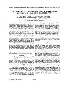
the output from road profilers is to collect profile data at test sections using a manual reference device, then compute roughness index, such as the international roughness index (IRI), from those data and compare the result with the output from the road profiler. Except for the first mentioned road profiler (RTRRMS), which measures directly the smoothness index (IRI), other profilers measure the road true profile, which is used to compute various smoothness indices using different methods. The accuracy of the computed indices greatly depends on the accuracy of the measuring equipment. Some of the most used indices are IRI [6], ride number (RN) [7], and half-car roughness index (HRI) [8]. In addition, there are other technologies, such as the longitudinal profile analyzer (LPA), which measures the longitudinal profile according to the standard NFP 98-218-3 and includes one or two single-wheel trailers towed at a constant speed by a car and a data acquisition system (Fig. 9). A ballasted chassis supports an oscillating beam holding a feeler wheel that is kept in permanent contact with the pavement by a suspension and damping system. The chassis is linked to the towing vehicle by a universal-jointed hitch. Vertical move-

삭제됨: 삭제됨: -

삭제됨: -

삭제됨:

M. Yousefzadeh et al. / Journal of Mechanical Science and Technology 24 (3) (2010) 743~754

Fig. 7. Lightweight profiler, courtesy of Traslogy Inc., used in a roundup in April 2004 at the Smart Road in Blacksburg [3].

Fig. 8. Dipstic 2000, face company [5].

Fig. 9. LPA developed by LCPC.

ments of the wheel result in angular displacement of the beam with respect to the horizontal arm of an inertial pendulum, independent of movements of the towing vehicle. This measurement is performed by an angular displacement transducer associated with the pendulum. Using accelerometer sensors on vehicles in order to improve their performances is becoming attractive for car manufacturers. Therefore, road measurement approaches, which utilize accelerometer sensors, are becoming interesting solutions for their justified economic advantages. This approach was introduced by González et al. They obtained the power spectral density (PSD) of a road profile using the data from accelerometers. Their methodology features a transfer function relating road profile PSD to PSD of accelerations [9]. In 2007, Hugo et al. developed a real-time condition-

745

triggered maintenance system to detect mine haul road defects and reconstruct the road profile using the measured response of a truck. The approach was based on measuring suspension forces and acceleration of the unsprung mass [10]. The accuracy of the above methods is affected by inaccurate vehicle manufacturer's data and insufficient degrees of freedom. Furthermore, both of these approaches demand formulating the inverse of a dynamic model. In order to avoid these problems, Ngwangwa et al. developed an artificial neural network (ANN) based technique to reconstruct the road profile. They used displacement responses of a quarter car model as inputs to a two-layer Narx network. They concluded that the technique is capable of reconstructing the road profile within a margin of error of 45%. They have also indicated that with other considerations, the error may decrease to 20% [11]. Usually ANN can perform system identification more accurately if sufficient input data are obtained. However, a large number of input variables may complicate the training process of ANN. Therefore, in this work, in order to achieve better accuracy in road profile reconstruction and also taking the economic advantages of accelerometer sensors, an ANN using seven vehicle acceleration variables were employed as inputs. There are four variables related to the vertical acceleration of the wheels and three variables related to the acceleration of the body (bounce, pitch, and roll). The model was implemented in MATLAB. Since the approach presented here is mainly based on a new concept, rather than directly utilizing a real operating measuring vehicle, a model of the vehicle in the ADAMS software was built and validated with existing experimental data. The results, derived from the analysis of the model, were used to teach the neural network and verify the estimation accuracy. The experimental data used for validating the ADAMS model had specific frequency components, whereas neural network training needed random data or data with a wider frequency range. Therefore, the experimental data used for the ADAMS model validation could not be used for ANN training. The data used in training and testing the ANN were obtained from the simulation of the ADAMS model, which was excited by road profiles generated via ADAMS. The applications of ANN based methods are rapidly increasing in various fields of science. They are able to approximate complicated systems. As for vehicle technology, neural network has contributed a lot of solutions to areas such as control and dynamic simulations. The following is a brief summary of some of the neural network contributions to the vehicular field. In 1993, Kageyama used a three-layer feed forward neural network to transform a group including 17 state variables of a vehicle model to four state variables of force. The outputs of the network were properly in agreement with the values resulting from the simulation [12]. In 1994, Palkovics and his team examined the ability of neural networks and also compared the feed forward and feedback neural network accuracy in simulation of a tire under vertical

746

M. Yousefzadeh et al. / Journal of Mechanical Science and Technology 24 (3) (2010) 743~754

dynamic load. Due to lack of experimental data for training the network, they used results from simulation of a magic formula (MF)-tire model, which was proposed by Pacejka and Takahashi in 1992 [13]. Their research showed feed forward methods are more accurate in estimation but not as robust as feedback methods. In conclusion, they showed that the majority of complicated models can be replaced with the tire model created by the neural network [14]. In 1994, Wurtenberger and Iserman used a feed forward eural network for obtaining a tire and vehicle model to study the lateral vehicle dynamics [15]. In 1996, Ghazizadeh and Fahim utilized a two-layer feed forward neural network to obtain a quasi-static roll model to study vehicle roll-over behavior. They used a vehicle model in which inputs were vehicle velocity and steering angle, and outputs were lateral acceleration, yaw rate, and quasi-static load transfer in the rear and front axles. They used network outputs with the number of time delays as feedback to the input [16]. In 1997, Pasterkamp and Pacjeka compared feed forward and radial basis networks to estimate the slip angle and the friction between the tire and road considering self-aligning torque and tire loads. They showed that although both networks perform reasonable estimation, feed forward networks are preferred because they have a smaller structure and are more robust. In addition, research pointed out that for determining the suspension system behavior, implementation of a suitably learned feed forward neural network is more appropriate than methods in which, to save on cost of measuring instruments, real-time complicated kinematic calculation has to be done [17].

2. Dynamic modeling of the vehicle As mentioned before, an off-road vehicle (jeep model) is modeled by the ADAMS/CAR software. ADAMS uses the geometric and dynamic parameters of the vehicle as input and creates the dynamic model equations. Furthermore, an embedded solver in ADAMS solves the generated equations. The front and rear suspension systems are of rigid type with helical springs and are illustrated in Figs. 10 and 11, respectively. As shown in Fig. 10, Axle 8 is carried by longitudinal Arms 6 and A-type control Arms 7. The A-arm absorbs lateral forces and longitudinal arms absorb the drive-off and braking forces. The longitudinal arms are linked to the body and axle by bushing joints. These bushings have translational and rotational stiffness in the x, y, and z directions. Coil spring 3 and vertical shock absorber 4 are shown in Fig. 10. The steering system is a recirculation ball type. Tie rod 5 is modeled as a link and connected to hob carrier 2 by a spherical joint. For modeling the steering system, the standard model of Pitman_Arm.tpl in ADAMS was used. A standard template known as Rigid_Chassis.tpl modeled the body. The tires were modeled with a standard model (i.e., Handling-Tire.tpl). The

Fig. 10. The front suspension system.

Fig. 11. The rear suspension system.

tire model was selected as Delft type using the MF-tire model. MF tire is the premier handling model available in ADAMS/Tire. In this model, the normal load FZ of the tire is calculated with FZ = CZ . z + K Z . z ,

(1)

where CZ, KZ, and z stand for vertical damping, vertical stiffness, and deflection of the tire, respectively. The general form (sine version) of the formula can be expressed as Fxor y = D.sin[C .tan −1{Bx − E ( Bx − tan −1 ( Bx ))}]

(2)

The general form of the self-aligning moment Mz is calculated by M z = D.cos[C .tan −1{Bz − E ( Bz − tan −1 ( Bz ))}]

(3)

where Bx, y, or z is the stiffness factor (in the x, y, or z direction), C is the shape factor, D is the peak value, and E is the curvature factor [18].

3. Model validation After vehicle dynamic modeling, several four-post and handling tests were performed to investigate the handling and ride performances of the vehicle. The simulation results were then compared with the time history measurements on the vehicle, which were carried out in the laboratory. Necessary modifica-

삭제됨: :

M. Yousefzadeh et al. / Journal of Mechanical Science and Technology 24 (3) (2010) 743~754

tions in the model parameters were made to achieve close agreement with the test results. The springs of the front suspension were assumed to be linear, and their stiffness was found from the static bench test. In rear suspension, nonlinear springs were used. Figure 12 shows the load deflection for the rear suspension based on the results from the bench test results. The force-velocity characteristics of the front and rear dampers were obtained from spring and damper bench tests and are shown in Fig. 13. The vehicle parameters are provided in Table 4. In the laboratory, two accelerometer sensors were applied to measure the vertical acceleration: sensor No. 1 (placed on the body, over the front-left part of the wheel) and sensor No. 2 (located under the driver's seat). In addition, optical sensors were employed to measure the pitch and roll angles. The positions of the sensors are shown in Figs. 14 and 15. Figure 16 shows the vehicle equipped with the measurement system and the four-post actuators. Comparison of the results from dynamic simulation and fourpost test, as shown in Figs. 17-19, revealed an acceptable correspondence between the results in both simulation and test. The vehicle model is reasonably accurate. As mentioned earlier, there are some differences between simulation and test results that could have originated from the following:

(a) The position of accelerometer sensor No. 1

(b) The position of accelerometer sensor No. 2 Fig. 14. The accelerometer position.

Fig. 12. Force versus displacement curve for the spring of the rear suspension.

Front Damper Rear Damper

2250 1500

Force (N ) -1000

Fig. 15. Optical sensor for measuring the body roll.

3000

750

-750

-500

0 -250 0 -750

250

500

750

1000

-1500 Velocity (mm/s)

Fig. 13. Force vs. velocity curve for the dampers of the front and rear suspension.

Fig. 16. Measuring system in the four-post laboratory.

747

748

M. Yousefzadeh et al. / Journal of Mechanical Science and Technology 24 (3) (2010) 743~754

(a) Simulation results

(a) Simulation results

(b) Experimental results (b) Experimental results Fig. 17. Pitch angle responses to the swept frequency input (0.5–1 Hz and amplitude of 20 mm) applied on the rear axle.

(a) Simulation results

Fig. 19. Acceleration responses to the opposite wheel travel input (pitch motion of 2 Hz and amplitude of 20 mm).

Fig. 20. The full-vehicle model in ADAMS.

● The inflexibility of the vehicle body model (rigidity). ● Nonlinear dynamic behavior of springs and dampers due to the contact with bumpers in reality, which were ignored in the model. As mentioned above, in the ride performance simulation and in order to choose the subsystem, the tire model was selected as Delft type and the four wheels were locked by constraints that prevented the forward and backward movements of the vehicle. The full-vehicle model is shown in Fig. 20. (b) Experimental results Fig. 18. Acceleration responses according to opposite wheel travel input (roll motion, 1 Hz, and amplitude of 30 mm).

4. Network architecture and training algorithm Neural networks are composed of simple elements operat-

M. Yousefzadeh et al. / Journal of Mechanical Science and Technology 24 (3) (2010) 743~754

ing in parallel. These elements are inspired by biological nervous systems. As in nature, the network function is determined largely by the connections between elements. Neural networks can be trained to perform a particular function by adjusting the values of the connections (weights) between elements. Commonly they are adjusted, or trained, so that a particular input leads to a specific target output. A one-layer network with R input elements and S neurons is shown in Fig. 21. In this network, each element of the input vector p is con-

Fig. 21. A one-layer neural network.

Fig. 22. A three-layer network.

Fig. 23. A three-layer network in abbreviated notation.

749

nected to each neuron input through the weight matrix W. The ith neuron has a summer that gathers its weighted inputs and bias to form its own scalar output n (i). The various n (i) taken together form an S-element net input vector n. Finally, the neuron layer outputs form a column vector a. The input vector elements enter the network through the weight matrix W, ⎡ w1,1 ⎢w 2,1 W =⎢ ⎢ ⎢ ⎢⎣ wS ,1

w1,2 … w1, R ⎤ w2,2 … w2, R ⎥⎥ ⎥ ⎥ wS ,2 … wS , R ⎥⎦

(4)

A network can have several layers. Each layer has a weight matrix W, a bias vector b, and an output vector a. Fig. 22 shows a three-layer network with R1 inputs, S1 neurons in the first layer, S2 neurons in the second layer, etc. The outputs of each intermediate layer are the inputs to the following layer. Thus, layer 2 can be analyzed as a one-layer network with S1 inputs, S2 neurons, and an S2×S1 weight matrix W2. The input to layer 2 is a1; the output is a2. The layers of a multilayer network play different roles. A layer that produces the network output is called an output layer. All other layers are called hidden layers. Figure 23 shows the three-layer network in abbreviated notation.

750

M. Yousefzadeh et al. / Journal of Mechanical Science and Technology 24 (3) (2010) 743~754

Fig. 24. Neural network configuration in the MATLAB software.

Fig. 25. Neural network block configuration.

Choosing an appropriate architecture of ANN is dependent on the type of system being modeled. In this work, the MATLAB software was used to model the intended ANN. As shown in Fig. 24, the inverse of a vehicle model was used to construct the ANN model, where the inputs were accelerations of a vehicle moving along a road and the outputs were the road profiles. The network is a dynamic ANN. In addition to the vehicle accelerations, the delayed version of the vehicle accelerations and the road profiles were also input to the ANN block. Figure 25 also demonstrates the ANN block in Fig. 24. The number of hidden layers and their nodes is an arbitrary parameter that cannot be determined according to a specified rule. In other words, an optimized network size can be achieved using trial and error and by considering the accuracy of the results and the training convergence speed. In this work, a network including two hidden layers with six hyperbolic tangent sigmoid (tansig) transfer function nodes and an output layer with linear transfer function nodes was created (Fig. 25). The outputs of the network were four road profiles related to each of the vertical displacements of the wheels during the vehicle trip. The network input consisted of two groups. The first group, called independent input, consisted of seven vehicle accelerations. The second group, dependent input, was the feedback of the network output and independent input, both with one and two delay elements. A dependent input was used because state variables in a dynamic system depend not only on the current inputs of the system but also on the state variables in previous time. In this model, several different delays and their combinations were analyzed, and, finally, the combination of one and two delays was found to be suitable. Neural networks adjust the values of weights and biases through a process that is referred to as a learning rule or training algorithm. The three training algorithms that are most suitable for function approximation are the Quasi-Newton, Scaled Conjugate Gradient, and Levenberg-Marquardt methods. Each of these methods was studied for training the network, and, finally, the Levenberg-Marquardt, which approximated with best accuracy, was chosen. The Levenberg-

Marquardt algorithm was designed to approach second-order training speed without having to compute the Hessian matrix. The Levenberg-Marquardt algorithm adjusts the weights by using the following equation: Wnew = Wold + ( J T J + λ I ) J T e (Wold ) −1

(5)

where I is the identity matrix, e(Wold) is an error vector at the current point, Wnew is the weight at the next point in the training procedure, J is the Jacobian matrix given by the partial derivative ∂ e(Wold)/ ∂Wold and λ is a parameter that governs the step size. The value of λ varies during network training.

5. Training data collection Network training data were gathered using the vehicle dynamic model in the ADAMS software. Two road profiles, generated in ADAMS, excited the front wheels. The other two road profiles for exciting the rear wheels were mostly similar to those of the front wheels but with some delays caused by the distance between the front and rear axles of the vehicle. These four road profiles with a specified vehicle velocity were applied to the vehicle model to derive seven accelerations, including three accelerations of the body (roll, bounce, and pitch) and four accelerations of the wheels. The generated road profiles were considered as network output training data. Input training data consisted of independent and dependent data, which were introduced in the previous section.

6. Training and testing the network For training and testing the network, road profiles similar to the types E and F of ISO 8608 standard [19] were used. As shown in Table 1, four groups of road profiles were created. Each of the road profiles consisted of four series of data for exciting the wheels of the vehicle in the ADAMS software. The road profiles were originally 1000 m long, but with considering 2.3 m distance between the rear and front axles, 997.7

삭제됨:

M. Yousefzadeh et al. / Journal of Mechanical Science and Technology 24 (3) (2010) 743~754

m of road profiles were used. Furthermore, the frequency content of the road profiles was around 0.1-1 cycles/m, as was intended from the beginning. After applying the roads to the vehicle at 30 m/s speed and deriving the accelerations, the transient span of the acceleraTable 1. Road profiles used for training and testing the network. Road profile No.

Road type

1

E

Application Training

2

F

Training

3

E

Test

4

F

Test

Table 2. Combination sets used for evaluating the networks. Combination No. 1

Training set

Testing set

Road Profile No. 1

Road Profile No. 3

2

Road Profile No. 2

Road Profile No. 4

3

Road Profile No. 2 1st Road Profile No. 1, 2nd Road Profile No.2 1st Road Profile No. 1, 2nd Road Profile No.2

Road Profile No. 3

4 5

Fig. 26. Combination No. 1.

Fig. 27. Combination No. 1.

Road Profile No. 4 Road Profile No. 3

751

tions should be removed to have a proper network training. Therefore, nearly 960 m of road profiles were used. As shown in Table 2, five combinations of road data from Table 1 with their corresponding accelerations were used to train and test five different networks. The transient parts of the data were removed before training and testing the network. All of the acceleration data were obtained with 30 m/s speed. The performance of the network can be studied more carefully by a statistical function, PSD, which is common for studying the frequency contents of road profiles. Figures 2635 show the left side estimated and target (real) road profiles in time and frequency domains (PSD). For better visibility of road profiles, the figures illustrate a zoomed portion of the road. The straight lines in the figures of PSD of road profiles are boundaries for road types recommended by the ISO 8608 standard. Figures 26-35 indicate the networks were quite successful in predicting the target profile. Obviously, the longer the wavelength content is in the road profile, the larger the geometric elevation is. Because in this study the longest wave in the road profile was considered to be 1 m, PSD results seem to be rather smooth for E and F road types. In order to investigate the accuracy of estimation, the corre-

Fig. 28. Combination No. 2.

Fig. 29. Combination No. 2.

752

M. Yousefzadeh et al. / Journal of Mechanical Science and Technology 24 (3) (2010) 743~754

Fig. 33. Combination No. 4.

Fig. 30. Combination No. 3.

Fig. 34. Combination No. 5.

Fig. 31. Combination No. 3.

Fig. 35. Combination No. 5.

lation factors between estimated and real road profiles were calculated. The following formula shows the correlation factor computation used in this work for two signals x and y: r= Fig. 32. Combination No. 4.

∑ {( x − x ).( y − y )} . ∑ {( x − x ) .( y − y ) } 2

2

(6)

753

M. Yousefzadeh et al. / Journal of Mechanical Science and Technology 24 (3) (2010) 743~754

Table 3. Correlation factor of actual and PSD of road profiles. Correlation Correlation factor factor of the road PSD of road profiles profiles 0.95 0.96

Combination No.

Training road type

Testing road type

1

E

E

2

F

F

3

F

E

4

E, F

F

5

E, F

E

0.81

0.98

Table 4. Full-vehicle model parameters. Parameter

Value

Front Suspension Stiffness

22500 N/m

Rear Suspension Average Stiffness

55720 N/m

Bushings Translational Stiffness (x or y direction)

45x105 N/m

0.99

Bushings Translational Stiffness (z direction)

45x104 N/m

0.80

0.98

Bushings Rotational Stiffness (Around x or y axis)

45 N.m/deg

0.82

0.99

Bushings Rotational Stiffness (Around z axis)

0.8 N.m/deg

Tire Vertical Stiffness

220 KN/m

Tire Vertical Damping

300 N.s/m

0.81

x and y are the mean values of x and y. Table 3 shows the correlation factor between the estimated and target road profiles. All of the combinations indicate road profile PSDs have higher correlation in comparison to the real road profiles (in time domain) except for combination No. 1, which shows a higher correlation of the real road profile. Combinations No. 4 and No. 5 used road profiles of types E and F for training. They were created to study if any noticeable changes in estimation accuracy in comparison to other combinations can be found. However, as shown in Table 3, no major differences were found between different combinations. In addition, through the various training and testing of neural networks, it was found that proper estimation requires the training road data to be rougher than the estimated road profiles.

7. Conclusion In this paper, the idea of road profile estimation using neural network algorithm is presented. Due to lack of equipment, such as a four-post laboratory and a vehicle provided with accelerometers and accurate distance measuring system, a full validated ride model in the ADAMS software was used for simulations. Furthermore, five neural networks with the same configuration were built in the MATLAB software and trained and tested with five different data sets. The results from comparison between estimated road by ANN and the target road generated by ADAMS (i.e., used for exciting the model) show that the ANNs were quite capable of estimating the road profiles especially in the form of PSD. In contrast to road profilers, which utilize a number of expensive distance laser sensors, the presented configuration features only seven accelerometers, which are less expensive than laser sensors. The model used in this research in the ADAMS software, like in most of the other methods, was a ride model, which does not take cornering effect into account. Furthermore, in this research, any transient parts of the data resulting from short-term cornering or initial movement were omitted. However, if an application needs to consider the data during cornering, it has to lower its speed down to a value that would not skew the results, so that the roll and yaw (vehicle’s angular movement around its vertical axis) motion of the vehicle resulting from cornering is negligible. Also, in the ADAMS software, handling should be chosen instead of ride

Front Axle Load

827 kgf

Rear Axle Load

783 kgf

Total Vehicle Mass

1610 kg

Pitch Moment of Inertia

1949 kg.m2

Roll Moment of Inertia

569.2 kg.m2

Yaw Moment of Inertia

2467 kg.m2

Wheel Base

2.28 m

simulation option and consequently yaw motion acceleration data should be included as well as other vehicle’s accelerations affected by cornering in the estimation process. Using these solutions, the neural network can be trained with the data involving cornering effects. In the next stage of this research, using road data including frequency contents with much longer wavelengths is planned to identify the effect of profiles’ frequency contents and vehicle speed on estimation accuracy.

References [1] American Society of Testing and Materials, Standard Terminology Relating to Vehicle Pavement Sections, ASTM E867, Annual Book of ASTM Standards, 4.03 (2000). [2] R. W. Perera and S.D. Kohn, Issues in Pavement Smoothness: A Summary Report, Final Report, NCHRP Project 2051 [01], Transportation Research Board, Washington D.C., (2002). [3] American Society of Testing and Materials, Standard Test Method for Measuring the Longitudinal Profile of Traveled Surfaces with an Accelerometer Established Inertial Profiling Reference, ASTM E950, Annual Book of ASTM Standards, 4.03 (2004). [4] American Society of Testing and Materials, Standard Test Method for Measuring Pavement Roughness Using a Profilograph, ASTM E1274, Annual Book of ASTM Standards, 4.03, (2008). [5] American Society of Testing and Materials, Standard Test Method for Measuring Road Roughness by Static Level Method, ASTM E1364, Annual Book of ASTM Standards, 4.03 (2000). [6] American Society of Testing and Materials, Standard Practice for Computing International Roughness Index of Roads from Longitudinal Profile Measurements, ASTM E1926,

754

M. Yousefzadeh et al. / Journal of Mechanical Science and Technology 24 (3) (2010) 743~754

Annual Book of ASTM Standards, 4.03 (2003). [7] American Society of Testing and Materials, Standard Practice for Computing Ride Number of Roads from Longitudinal Profile Measurements Made by an Inertial Profile Measuring Device, ASTM E1489, Annual Book of ASTM Standards, 4.03 (2007). [8] M. W. Sayers and S. M. Karamiahas, The Little Book of Profiling, University of Michigan Transportation Research Institute, (1998). [9] A. González, E. J. O’brien, Y. Li and K. Cashell, The use of vehicle acceleration measurements to estimate road roughness, Vehicle System Dynamics, 46 (2008) 483-499. [10] Daniel Hugo, Stephan P. Heyns, Roger J. Thompson and Alex T. Visser, Condition-Triggered Maintenance for Mine Haul Roads with Reconstructed-Vehicle-Response to Haul Road Defects, Journal of the Transportation Research Board, (2007) 254-260. [11] Harry M. Ngwangwa, P.Stephan Heyns, Kobus F. J. Labuschange and Grant K. Kululanga, An Overview of the Neural Network Based Technique for Monitoring of Road Condition via Reconstructed Road Profiles, Proc. of the 27th Southern African Transport Conference, ISBN No.: 978-1920017-34-7, (2008). [12] I. Kageyama, On a Control of Tire Force Coefficient for Vehicle Handling with Neural Network System – Estimation for Load Rate of Tire Forces, 13th IAVSD Symposium on Dynamics of Vehicles on Roads and Tracks, Chengdu, Sichuan, China, (1992) 31-40. [13] H. B. Pacejka and T. Takahashi, Pure Slip Characteristics of Tires on Flat and Undulated Road Surfaces, Proc. Int. Symp. Advanced Vehicle Control, SAE, Japan, No. 923064, (1992) 360-365. [14] L. Palkoviks, M. El-Gindy and H. B. Pacejka, Modeling of the Cornering Characteristics of Tires on an Uneven Road Surface, Dynamic Version of the "Neuro-Tire", Int. Journal of Vehicle Design, 15 (1/2) (1994) 189-215.

[15] M. Wurtenberger and R. Iserman, Model Based Supervision of Lateral Vehicle Dynamics, Proc. American Control Conference, 1 (1994) 408-412. [16] A. Ghazizadeh and A. Fahim, Neural Network Representation of a Vehicle Model: "Neuro-Vehicle", Int. J. of Vehicle Design, 17 (1) (1996) 55-75 [17] W. R. Pasterkamp and H. B. Pacejka, Application of Neural Networks in the Estimation of Tire/Road Friction Using the Tire as Sensor, SAE, No. 971122, (1997). [18] ADAMS/Tire Help, ADAMS/CAR Software. [19] Mechanical Vibration-Road Surface Profiles-Reporting of Measured Data, International Organization for Standardization, ISO 8608, (1995).

Mahdi Yousefzadeh received his B.S. degree in Mechanical Engineering from Mazandaran University (currently called Babol Noshirvani University of Technology), Iran, in 2000. He then received his M.S. degree from K.N. Toosi University of Technolgy, Iran, in 2003.

Shahram Azadi received his B.S. and M.S. degrees in Mechanical Engineering from Sharif University of Technology, Iran, in 1988 and 1992, respectively. He then received his Ph.D. from Amirkabir University of Technology, Iran, in 1999. Dr. Azadi is currently a Professor in the faculty of Mechanical Engineering at K.N.Toosi University of Technology in Tehran, Iran.