from an alphabet that has at least as many letters as features that need to be ... can be encoded in a different colours, intensities, shapes, ... or a combination of ...
Robot positioning using structured light patterns suitable for self calibration and 3D tracking Kasper Claes, Herman Bruyninckx Department of Mechanical Engineering, Katholieke Universiteit Leuven Celestijnenlaan 300B, 3001 Leuven (Heverlee), Belgium {first.last}@mech.kuleuven.be
Abstract— We study the control of a robot arm with an eye-in-hand camera, using structured light with a projector in a fixed but unknown position. Based on the theory of perfect maps, we propose a deterministic method to generate patterns independent of the relative 6D orientation between the camera and the projector, with any alphabet size and minimal Hamming distance between the codes. This independence makes self calibration using a known robot motion possible, and removes the need for less robust calibration grids. Patterns that are large enough for controlling a robotic arm are generated with error correcting capabilities. The experiments show the controlled motion of an industrial robot to a chosen position near a non-planar object, using a projector-camera calibration. This provides a wider baseline and hence more robustness than structure from motion.
I. I NTRODUCTION Positioning a robot with stereo vision (or similarly structure from motion) depends on features visible from several points of view. However these are not always present. Structured light solves this problem providing artificial visual features on the scene independent of the scene, easing considerably a difficult part of stereo vision: the correspondence problem. The structured light technique used replaces one camera of a stereo vision system by a projector. The other camera is attached to the end effector of a 6DOF robotic arm. This paper focusses on how the correspondences are determined: we propose an algorithm with reproducable results (as opposed to the random approach by Morano [1]) that generates a pattern suitable for robotic arm positioning as shown in figure 1. We choose this setup because current projectors do not allow the projector to be moved around: the hot lamp filament can break from vibrations. Therefore in our experiments the projector has a static position: a projectorto-hand setup. The camera on the other hand is moving rigidly with the end effector: an eye-in-hand setup avoids occlusions and can percieve more detail as the robot is approaching the scene. The projected pattern only uses local information and is therefore robust against partial occlusions, possibly due to the robot itself. Before calibration there is no information on the relative rotation between camera and projector. A gray code projection pattern in two directions with a calibration grid as presented by Inokuchi [2] can cope with this unknown rotation. But, for robustness reasons, we plan on self calibrating the setup. Therefore a method to generate 2D
patterns is designed such that this the correspondences are independent of the unknown relative orientation, as in the work of Adan [3] for which we propose an improval in section II. In addition larger minimal Hamming distances between the projected codes provide the pattern with error correcting capabilities. All correspondences can be extracted from one image: the pattern is suitable for tracking a moving object.
xc zc
zp
yc
xp projector
yp Fig. 1.
Schematic setup
Pages [4] chooses the same setup for image based visual servoing (IBVS): the depth estimation is rough since IBVS is robust against depth errors. He points out that using depth from a calibrated setup would improve performance. Structure from motion by tracking features between several poses of the camera calibrates the setup: the viewpoints are not separated in space but in time. Pages does not calibrate the projector-camera pair: the projector is only a feature generator to ease the correspondence problem. But the baselines in optical flow are small, and the larger the baseline the better triangulation conditioning. Hence we calibrate using the wider projector-camera baseline. Section II deals with the projected pattern and section III shows the robotics experiments.
II. T HE CORRESPONDENCE PROBLEM Epipolar geometry eases the correspondence problem by limiting the points in an image that can possibly correspond to a point in the other image to a line, hence reducing the search space from 2D to 1D. Even that 1D problem can be difficult to impossible when little or no texture is present: e.g. visual servoing of a mobile robot along a uniformly coloured wall is not possible without a projector. 1D structured light patterns make use of the epipolar constraints by projecting vertical lines. If the camera stands beside the projector, the intersection of the epipolar lines in the camera image and the projection planes is conditioned better than when the lines would be projected horizontally. In a setup where the projector is on top or below the camera, horizontal lines would be best. However, in order to calculate the extrinsic parameters needed for exploiting epipolar geometry, 2D correspondences between camera and projector images are necessary. So during a calibration phase typically both horizontal and vertical patterns are projected, after calibration only stripes in one direction. Associating the pixels in camera and projector image can be done using time multiplexing or based on one image, as summarized by Salvi [5]. In the time based approaches, the scene has to remain static as multiple images are needed to define the correspondences. Our approach aims at moving scenes, so we choose a method based on a single image. A 2D pattern is not only usefull for the initial calibration of this setup but also online, since a constantly changing baseline requires the extrinsic parameters to be adapted constantly. To be able to define the position in the projector image of all the projected features observed by the camera, each projected feature needs to correspond to a unique code from an alphabet that has at least as many letters as features that need to be recognized. Morano [1] separates the letter in the alphabet of each element of the matrix, and the representation of that letter. The representation can be encoded in a different colours, intensities, shapes, ... or a combination of these elements. Projecting an evenly spread matrix of features with m rows and n columns requires an alphabet of size n.m. E.g. for a 640 × 480 camera (assuming the best case scenario that the whole projected scene is barely visible), projecting a feature every 10 pixels requires a 64 × 48 grid: over 3000 identifiable elements. Trying to achieve this using for example a different colour for each feature (direct coding) – or intensity in the grayscale case – is not realistic as the system would be too sensitive to noise. Projecting more complex features, like several spots next to each other that define one code, drastically reduces the size of the alphabet needed. But as the projected features become larger, it’s more likely that parts of them are invisible due to for example depth discontinuities. A solution is to share spots nearby: exploit spatial neighbourhood.
A. 2D Spatial neighbourhood Spatial neighbourbood takes neighbouring features into account to reduce the number of identifiable elements needed for a constant amount of codes, Salvi [5] made an overview of work in this field. For 1D patterns, a De Bruijn sequence can be used: a cyclic sequence from a given alphabet (size a) for which every possible subsequence of a certain length is present exactly once. A possible extension in 2D is a matrix of elements. Then the theory of perfect maps can be used: a perfect map has the same property as a De Bruijn sequence, but in 2D: for a certain submatrix and matrix size, every submatrix occurs only once in a matrix of elements from a given alphabet. These perfect maps can be constructed in several ways. Etzion [6] for example uses De Bruijn sequences: the first column is a De Bruijn sequence, and the next columns consist of cyclic permutations of that sequence, each column shifted one position in the sequence. A disadvantage of this technique is that there is a fixed relation between the size of the desired submatrix w × w and the size of the entire matrix r×c, namely r = c = aw . rr rr rr rr rr rr rr rr r rr rr rr rr rr rr rr rr r rr rr rr rr rr rr rr rr r rr rr rr rr rr rr rr rr r rr rr rr rr rr rr r rr rr rr rr rr rr r rr rr rr rr rr rr rr rr r rr rr rr rr rr rr rrr rr rr rr rr rr rr rr rr rrr rr rr rr rr rr rr rr rr rrr rr rr rr rr rr rr rr rr rrr rr rr rr rr rr rr rrr rr rr rr rr rr rr rrr rr rr rr rr rr rr rr r rr rr rr rr rr rr rr rr r rr rr rr rr rr rr rr rr r rr rr rr rr rr rr rr rr r rr rr rr rr rr rr rr rr r rr rr rr rr rr rr r rr rr rr rr rr rr r rr rr rr rr rr rr rr rr r rr rr rr rr rr rr rrr rr rr rr rr rr rr rr rr rrr rr rr rr rr rr rr rr rr rrr rr rr rr rr rr rr rr rr rrr rr rr rr rr rr rr rrr rr rr rr rr rr rr rrr rr rr rr rr rr rr rr r rr rr rr rr rr rr rr rr r rr rr rr rr rr rr rr rr r rr rr rr rr rr rr rr rr r rr rr rr rr rr rr rr rr r rr rr rr rr rr rr r rr rr rr rr rr rr r rr rr rr rr rr rr rr rr r rr rr rr rr rr rr rrr rr rr rr rr rr rr rr rr rrr rr rr rr rr rr rr rr rr rrr rr rr rr rr rr rr rr rr rrr rr rr rr rr rr rr rrr rr rr rr rr rr rr rrr rr rr rr rr rr rr rr r rr rr rr rr rr rr rr rr r rr rr rr rr rr rr rr rr r rr rr rr rr rr rr rr rr r rr rr rr rr rr rr rr rr r rr rr rr rr rr rr r rr rr rr rr rr rr r rr rr rr rr rr rr rr rr r rr rr rr rr rr rr rrr rr rr rr rr rr rr rr rr rrr rr rr rr rr rr rr rr rr rrr rr rr rr rr rr rr rr rr rrr rr rr rr rr rr rr rrr rr rr rr rr rr rr rrr rr rr rr rr rr rr rr r rr rr rr rr rr rr rr rr r rr rr rr rr rr rr rr rr r rr rr rr rr rr rr rr rr r rr rr rr rr rr rr rr rr r rr rr rr rr rr rr r rr rr rr rr rr rr r rr rr rr rr rr rr rr rr r rr rr rr rr rr rr rrr rr rr rr rr rr rr rr rr rrr rr rr rr rr rr rr rr rr rrr rr rr rr rr rr rr rr rr rrr rr rr rr rr rr rr rrr rr rr rr rr rr rr rrr rr rr rr rr rr rr rr r rr rr rr rr rr rr rr rr r rr rr rr rr rr rr rr rr r rr rr rr rr rr rr rr rr r rr rr rr rr rr rr rr rr r rr rr rr rr rr rr r rr rr rr rr rr rr r rr rr rr rr rr rr rr rr r rr rr rr rr rr rr rrr rr rr rr rr rr rr rr rr rrr rr rr rr rr rr rr rr rr rrr rr rr rr rr rr rr rr rr rrr rr rr rr rr rr rr rrr rr rr rr rr rr rr rrr rr rr rr rr rr rr rr r rr rr rr rr rr rr rr rr r rr rr rr rr rr rr rr rr r rr rr rr rr rr rr rr rr r rr rr rr rr rr rr rr rr r rr rr rr rr rr rr r rr rr rr rr rr rr r rr rr rr rr rr rr rr rr r rr rr rr rr rr rr rrr rr rr rr rr rr rr rr rr rrr rr rr rr rr rr rr rr rr rrr rr rr rr rr rr rr rr rr rrr rr rr rr rr rr rr rrr rr rr rr rr rr rr rrr rr rr rr rr rr rr rr r rr rr rr rr rr rr rr rr r rr rr rr rr rr rr rr rr r rr rr rr rr rr rr rr rr r rr rr rr rr rr rr rr rr r rr rr rr rr rr rr r rr rr rr rr rr rr r rr rr rr rr rr rr rr rr r rr rr rr rr rr rr rrr rr rr rr rr rr rr rr rr rrr rr rr rr rr rr rr rr rr rrr rr rr rr rr rr rr rr rr rrr rr rr rr rr rr rr rrr rr rr rr rr rr rr rrr rr rr rr rr rr rr rr r rr rr rr rr rr rr rr rr r rr rr rr rr rr rr rr rr r rr rr rr rr rr rr rr rr r rr rr rr rr rr rr rr rr r rr rr rr rr rr rr r rr rr rr rr rr rr r rr rr rr rr rr rr rr rr r rr rr rr rr rr rr rrr rr rr rr rr rr rr rr rr rrr rr rr rr rr rr rr rr rr rrr rr rr rr rr rr rr rr rr rrr rr rr rr rr rr rr rrr rr rr rr rr rr rr rrr rr rr rr rr rr rr rr r rr rr rr rr rr rr rr rr r rr rr rr rr rr rr rr rr r rr rr rr rr rr rr rr rr r rr rr rr rr rr rr rr rr r rr rr rr rr rr rr r rr rr rr rr rr rr r rr rr rr rr rr rr rr rr r rr rr rr rr rr rr rrr rr rr rr rr rr rr rr rr rrr rr rr rr rr rr rr rr rr rrr rr rr rr rr rr rr rr rr rrr rr rr rr rr rr rr rrr rr rr rr rr rr rr rrr rr rr rr rr rr rr rr r rr rr rr rr rr rr rr rr r rr rr rr rr rr rr rr rr r rr rr rr rr rr rr rr rr r rr rr rr rr rr rr rr rr r rr rr rr rr rr rr rr rr rr rr rr rr rr r rr rr rr rr rr rr rr rr r rr rr rr rr rr rr rr rr rr rr rr rr rr rr rr rr rr rr rr rr rr rr r rr rr rr rr rr rr rr rr rr rr rr rr rr rr rr r rr rr r rr rr r rr rr rr rr rr rr rrr rr rr rrr rr r rr rr rr rr rr rr rr rr r rr rr r rr rr r rr rr rr rr rr rr rrr rr rr rrr rr r rr rr rr rr rr rr rr rr rr rr rr rr rr Fig. 2. top: result with w = 3, a = 6, h = 3: 2352 codes (44 × 58), bottom: same but h = 5: 88 codes (10 × 13)
B. Pattern rotation In the experiments we calibrate using a calibration grid and gray code patterns in 2 directions. Because of the lower robustness of the associated algorithms, and the need for online updating of extrinsic parameters, a self calibration procedure is planned. Starting from an uncalibrated system, the rotation between camera and projector is unknown. Therefore each submatrix of the projected pattern can occur only once for any orientation. The construction as proposed by Etzion [6] does not have this property, which we will call rotational invariance, as can be proven by rotating each w × w submatrix over π2 , π and 3π 2 and then comparing it to all other submatrices: the same submatrices are found.
So, when the rotation is unknown perfect maps need to be constructed in a different way. The computational cost of simply testing all possible matrices is prohibitively expensive: ac ∗ r matrices have to be tested, for example for the modest case of an alphabet of only 3 letters (e.g. using colours: red, green, blue) and a 20 × 20 matrix, this yields about 10191 matrices to be tested. Morano [1] proposed a more efficient brute force method. First the top left w × w submatrix is randomly filled, then all w × 1 columns right of it are constructed such that the uniqueness property remains valid. Next all 1 × w rows beneath the top left submatrix are filled with random asignments, and afterwards every single new element determines a new code: the remaining elements are determined always ensuring uniqueness. If no solution can be found at a certain point (all a letters of the alphabet are exhausted), the algorithm is aborted and started over again with a different top left submatrix. In this way Morano can cope with any combination of w, r and c, but the algorithm is not meant to be rotationally invariant. We alter this algorithm in three ways: • Perfect maps imply square projected entities, so out of every spot with its 8 neighbours, 4 are closer and √ the 4 others are a factor 2 further. This means that the only restrictions that have to be satisfied are rotations over π2 , π and 3π 2 . Thus, while constructing the matrix, each element is compared using these 4 rotations. Each feature is now less likely to be accepted than in the Morano case, but the only 4 contraints keep the search space of all possible codes relatively big, increasing the chances of finding a valid perfect map. • At each step, a certain subset of elements needs to be chosen: the w × w elements of the top left submatrix in the beginning, the w elements when a new row of columns is started, or 1 element otherwise. Putting each of these matrix elements after one another yields a huge base a number. In the algorithm, this number always increases, so a perfect map candidate is never checked twice. We assume a depth-first search strategy: at each iteration the elements that can be changed at that point (size w2 ,w or 1) are increased by 1 base a, until the w × w submatrix occurs only once (considering the rotations). When increasing by 1 is no longer possible, we assign 0 to the changable elements and use backtracking to increase the previous elements. In this way only promising branches of the tree are searched until the leaves, and restarting from scratch is never needed. The size to the search space is only a ath of the space used by Morano, as the absolute value of each element of the matrix is irrelevant. Indeed, the matrix is only defined up to a constant term base a, as the choice of which letter corresponds to which representation (e.g.colour) is arbitrary. So we can assume the top left element of the matrix to be zero. Agreed that the remaining search space remains huge.
We construct the matrix without first determining the first w rows and first w columns. In this way, larger matrices can be created from smaller ones without the unnecessary constraints of these first rows and columns. No need for specifying the final number of columns or rows at the beginning of the algorithm either. At each increase in matrix size, w new elements are added to start a new column, and w to start a new row, then the matrix can be completed by adding one element at each time. Also, the aspect ratio is considered in this step, for example for a 1024×768 projector (aspect ratio 4:3), for every fourth new column no new row is added. After the calibration one could use a pattern without the extra constraint of the rotational invariance, and rotate this pattern according to the camera movement. But this implies more calculations online. Moreover, even when the scene is static, different points are reconstructed in function of the camera movement, complicating the pose estimation. Hence, we choose to use the rotational invariant pattern both for calibration and online tracking. C. Redundant encoding •
Two mean sources of errors are taken into account: • Low level vision: decoding of the representation (e.g.intensities) can be erroneous when the segmentation is unable to separate the projected features. • Scene 3D geometry: depth discontinuities can cause occlusion of part of the pattern. As explained in [1] the proposed pattern is able to deal with these discontinuities because every element is encoded w2 times: once for every submatrix it belongs to. A voting strategy is used here: for every element the number of correct positives are compared to the number of false positives. Robustness can be increased by increasing this signal to noise ratio: move the code of every submatrix further away from every other submatrix. In order to be able to correct n false decodings in a code, it’s Hamming distance h has to be 2n + 1. Only requiring each submatrix to be different from every other submatrix produces a perfect map with h = 1, and hence no error correction capability. Requiring for example 3 elements of every submatrix to be different from every other submatrix, makes the correction of one erroneous element possible. Or, to put it in voting terms: every element in a submatrix could be wrong, discarding each one of the w2 elements of the code at a time labels all elements of that submatrix w2 times. As each element is part of w2 submatrices, the confidence number (signal) can be as high as w4 . The larger w, the less local every code and the more potential problems with depth discontinuities. An even w is not useful, because in that case no element is located in the middle. w = 1 is direct encoding: not a realistic strategy. Therefore we choose w = 3. In the experiments, we choose a = 6 as it is a suitable value to produce perfect map suffiently large for this application.
The larger h the better, but the more restrictive the comparison between every two submatrices. The projected spots should not be too small as they cannot be robustly decoded anymore then. An element every 10 pixels seems a reasonable compromise. For a camera with VGA resolution, this means we need a perfect map of about 48 × 64. Requiring h = 3 in our technique quickly yields a satisfactory 44×58 result. With h = 5 the algorithm does not find a larger solution than 10 × 13 in the first minutes. To increase this map, a larger a would have to be chosen. With h = 1, the above algorithm produces a 203 × 268 perfect map in a few minutes: needlessly oversized for our application. Figure 2 illustrates a result of our algorithm. Pages [4] uses the same setup but does not consider what happens when the view of the pattern is rotated over more than π4 . There a standard Morano pattern of 20 × 20, h = 1, a = 3 is used. It would be interesting to be able to produce these patterns analytically. Etzion [6] did this, but the patterns are not rotationally invariant, square and of Hamming distance 1. D. Hexagonal maps Adan [3] uses a hexagonal pattern instead of a matrix. Each submatrix consists of a hexagon and its central point. This can be achieved by shifting the odd elements half a position down and making the odd columns one element shorter than the even columns. An advantage of this pattern is that the distance to all neighboors is equal. So, if precision is needed, this distance can be chosen as small as the smallest distance which is still robustly detectable for the low level vision. In the perfect map case, the corner elements of the squares are further away than for example the elements directly beside the center. Hence the chance of failure due to occlusion of part of the pattern is minimal in the hexagonal case, but not in the perfect map case. Also, the total surface used in the projector image can be made smaller than in the perfect map case. Say the distance between each row is d (the smallest distance permitted by vision) then the distance between each column √ is not d as in the perfect map case, but 23d , permitting a total surface reduction of 86.6%. These are two – rather small – advantages concerning accuracy. Adan uses colour and encodes every submatrix to be different if its number of elements in a the different colours is different: the elements are regarded as a set. The advantage of this presented in [3], is that it reduces the online computational cost. Indeed, one does not have reconstruct the orientation of each submatrix. His hexagonal pattern is therefore also rotationally invariant, which is a desired property in the context of a moving camera. The number of possible codes is a (for the central element) times the combination �with repetition to choose 6 elements out of a : a a+6−1 . For example, for a = 6 the number of 6 combinations is 2772, which is a rather small number since codes chosen from this set have to fit together in a matrix. Hence, Adan uses a slightly larger alphabet with a = 7, resulting in 6468 possibilities.
However, restricting the code to a set is not necessary to ensure rotational invariance without adding considerable online computational cost. It is sufficient to consider all codes up to a cyclic permutation. This is less restrictive while constructing the matrix and should allow the construction of larger matrices or matrices with larger Hamming distance between its codes. Since the code length l = 7 is prime, all cyclic permutations have length l, except when all elements of the code are the same, the length of the cyclic permutation is 1. Therefore, the l number of possible codes is a + a −a l , equal to 39996 for a = 6 or 117655 for a = 7, considerably larger than 2772 and 6468, and hence drastically increases the probability of finding a suitable hexagonal map. r rr r rr r rr r rr r rr r rr r rr r rr r rr r rr r rr r rr r rr r rr r rr r rr r rr r rr r rr r rr rrr rr rrr rr rrr rr rrr rr rrr rr rrr rr rrr rr rrr rr rrr rr rrr rr rrr rr rrr rr rrr rr rrr rr rrr rr rrr rr rrr rr rrr rr rrr rr rrr rr r rr r rr r rr r rr r rr r rr r rr r rr r rr r rr r rr r rr r rr r rr r rr r rr r rr r rr r rr r rr rrr rr rrr rr rrr rr rrr rr rrr rr rrr rr rrr rr rrr rr rrr rr rrr rr rrr rr rrr rr rrr rr rrr rr rrr rr rrr rr rrr rr rrr rr rrr rr rrr rr r rr r rr r rr r rr r rr r rr r rr r rr r rr r rr r rr r rr r rr r rr r rr r rr r rr r rr r rr r rr rrr rr rrr rr rrr rr rrr rr rrr rr rrr rr rrr rr rrr rr rrr rr rrr rr rrr rr rrr rr rrr rr rrr rr rrr rr rrr rr rrr rr rrr rr rrr rr rrr rr rrrrrrrrrrrrrrrrrrrr rr rr rr rr rr rr rr rr rr rr rr rr rr rr rr rr rr rr rr rr rr rr rr rr rr rr rr rr rr rr rr rr rr rr rr rr rr rr rr rr rrr rr rrr rr rrr rr rrr rr rrr rr rrr rr rrr rr rrr rr rrr rr rrr rr rrr rr rrr rr rrr rr rrr rr rrr rr rrr rr rrr rr rrr rr rrr rr rrr rr rrrrrrrrrrrrrrrrrrrr rr rr rr rr rr rr rr rr rr rr rr rr rr rr rr rr rr rr rr rr rr rr rr rr rr rr rr rr rr rr rr rr rr rr rr rr rr rr rr rr rr rr rr rr rr rr rr rr rr rr rr rrr rr rrr rr rrr rr rrr rr rrr rr rrr rr rrr rr rrr rr rrr rr rrr rr rrr rr rrr rr rrr rr rrr rr rrr rr rrr rr rrr rr rrr rr rrr rr rrr rr rr rr rr rr rr rr rr rr rr rr rr rr rr rr rr rr rr rr rr rr rr rr rr rr rr rr rr rr rr rr rr rr rr rr rr rr rr rr rr rr rr rr rr rr rr rr rr rr rr rr rr rr rr rr rr rr rr rr rr rr rr rr rr rr rr rr rr rr rr rr rr rr rr rr rr rr rr rr rr rr rr rr rr rr rr rr rr rr rr rr rr rr rr rr rr rr rr rr rr rr rr rr rr rr rr rr rr rr rr rr rr rr rr rrrrrrrrrrrrrrrrrrrrrrrrrrrrrrrrrrrrrrrr Fig. 3. left: result with w = 3, a = 6, h = 1: 950 codes (27 × 40), bottom: same but h = 3: 54 codes (8 × 11)
An algorithm similar to the one for perfect maps was implemented for the hexagonal case, but in our experiment 6 possible rotations have to be checked for every spot. This, in combination with a smaller neighbourhood, proves to be more restrictive: as can be seen in figure 3 the Hamming distance that can be reached for a pattern of a suitable size is lower. In figure 3 a 4:3 aspect ratio was used, and the columns are closer together than the rows as 8 explained before, leading to a factor of 3√ more columns 3 than rows. III. E XPERIMENTS A. pattern generation Below you find the results of the proposed algorithm for perfect map generation. All results are obtained within minutes. The tables show the number of potentially 1 reconstructed points and the size of the 2D array: a\h 2 3 4 5 6 7 8
1 108 (11 × 14) 910 (28 × 37) 6188 (70 × 93) 40950 (177 × 236) 53934 (205 × 270) 116230 (297 × 396) 131566 (316 × 421)
3 6 (4 × 5∗ ) 70 (9 × 12) 108 (11 × 14) 588 (23 × 30) 2352 (44 × 58) 4015 (57 × 75) 7154 (75 × 100)
5 2 (3 × 4∗ ) 6 (4 × 5∗ ) 15 (5 × 7) 48 (8 × 10) 88 (10 × 13) 88 (10 × 13) 88 (10 × 13)
Calculating for several days improves some of the results: a=4,h=3: 14x18; a=7,h=1: 372x496; a=7,h=5: 13x17. An * indicates that the search space was calculated exhaustively and no array with a bigger size can be found. Results for the hexagonal variant: 1 potentially
because the camera does not always observe all spots
a\h 2 3 4 5 6 7 8 14
1 24 (6 × 8) 77 (9 × 13) 216 (14 × 20) 260 (15 × 22) 950 (27 × 40) 1040 (28 × 42) 1040 (28 × 42) 2838 (45 × 68)
3 imposs. 12 (5 × 6) 35 (7 × 9) 54 (8 × 11) 54 (8 × 11) 96 (10 × 14) 96 (10 × 14) 96 (10 × 14)
5 imposs. imposs. 2 (3 × 4∗ ) 6 (4 × 5) 6 (4 × 5) 12 (5 × 6) 12 (5 × 6) 12 (5 × 6)
at a certain distance is a, and the height below this ray is a . b, then the projector height is increased by a factor 2 a+b
We compare the results to those published by Morano [1]. Although the proposed constraints (rotational invariance) are more restrictive, bigger arrays can be generated with smaller alphabets, and results are reproducible. Morano indicates which combinations of a and h are able to generate a 45 × 45 array. A ”v” in the table indicates that the algorithm was successful while an ”x” indicates failure. The maximum number of columns (and rows) in the array is reached within a few minutes. a\h 3 4 5 6 7 8
1 Morano v v v v v v
Fig. 4. Top left: image, top right: segmentation, bottom: reconstruction.
3 this v (49) v (85) v (172) v (367) v (449) v (460)
Morano x x x x x v
this x (10) x (17) x (31) x (42) v (73) v (116)
B. robot positioning In order to calculate the depth of the points in the scene, the intrinsic parameters of the projector and the camera, and the extrinsic parameters between them, have to be estimated. In the experiments we use a calibration grid. The only deviation from the pin hole model that is compensated for in camera and projector, is the one that has most influence on the reconstruction: radial distortion. One could choose to adapt the polynomial approximation model by Brown [7], but in order not to increase the dimensionality of the problem by adding more parameters to be estimated, we use the model proposed by Perˇs [8]. He proposes an analytical alternative for barrel distortion, based on the observation that parts of the image near the edges look like they could have been taken using a camera with a much smaller angle that is slightly tilted: − 2r f
ru = − f2 e − fr−1 , with f the principle distance. This e model is only useful for cameras that are not optically or electronically corrected for barrel distortion, which is the case for most industrial cameras. For the projector calibration, a binary gray code sequence of patterns is used as in [2], both in horizontal and vertical directions, maximising the Hamming distances between consecutive code words. The LCD components of most projectors are not mounted along the central ray of the lens, but in such a way that the projection is upwards: only the upper part of the lens is used. We need to take this into account during the calibration and the radial distortion correction: we use a virtual projector screen with a larger height, as mentioned by Koninckx [9]. When the height above the central ray
We implemented this procedure with the pattern of fig.2 with h = 3, w = 3, a = 6, using 3 colours and 2 intensities. First a colour/intensity calibration is performed in such a way that the distance between the colour and the intensity values of the spots in the camera image, which correspond to different letters of this alphabet, is as large as possible. This is necessary since both the camera and the projector have different non-linear reponse functions for each of the colour channels. The projected colours are not adapted to the colour of the scene at each point here: we assume that the scene is not very colourful. For an arbitrary scene this adaptation would have to be done, as proposed in the work of Caspi [10]. Also, no compensation for specular reflections is present at the moment: we assume lambertian reflectivity. The camera image is converted to the HSV colour space. Assuming that the intensity of the ambient light is negligible compared to the intensity of the projector light, blob detection can be applied to the V-channel. The median of the H and V-values of each blob is used to segment the image. The sizes of the projected blobs are adapted to the size that is most suitable from the camera point of view for each position of the robot end effector: not too small which would make them not robustly detectable, and not to large which would compromise the accuracy. Since invariance to only 4 rotations is imposed, we need to find the orientation of the two orthogonal directions to the 4 neighbours of each spot that are closest, and the orientation of the two orthogonal directions to the 4 neighbours that are furthest away (the diagonals). This is done spot by spot. Then an EM estimator uses the histogram of these orientations to automatically determine the angle which will best separate the nearest and the furthest neighbours. This angle is then used to construct the graph that connects each spot to both kinds of neighbours. First the closest four spots in the expected direction are localized. Then the location of the diagonal neighbours is predicted, using the vectors between the central and the
closest four spots. The location of the diagonal neighbours is then corrected choosing the spots that are closest to the prediction. Now the consistency of the connectivity graph is checked. Consider a rotated graph such that one of the closest neighbour orientations points upwards. Then, the upper neighbour needs to be the left neighbour of the upper right neighbour, and at the same time the right neighbour of the upper left neighbour. Similar rules are applied for all neighbouring spots. All codes that do not comply to these rules are rejected. f ee f cam fb
Fig. 5.
Involved frame transformations and robot setup.
Now each valid string of letters of the alphabet can be decoded. Since this will be an online process at the highest possible frequency, efficiency is important. Therefore, the base 6 strings of all possible codes in all 4 orientations are quicksorted in a preprocessing step. During online processing, the decoded codes can be found using binary search of the look up table: this only has a complexity of O(log n). We use voting to correct a single error. If a code is found in the LUT, then the score for all elements of the code in the observed colour is increased by 9: once for each hypothesis that one of the neighbouring spots and the central spot is erroneous. If the code is not found, then for each of the 9 elements we try to find a valid code by changing only one of the elements to any of the remaining letters in the alphabet. If such code can be found, we increase the score for that colour of that spot by one. Then we assign the colour to the spot that has the highest vote, and decode the involved spots again. The correspondences are then used for epipolar reconstruction of the scene, as shown in fig.4: this implies solving a homogeneous system of equations for every
point, using an SVD method. Using the 3D point cloud, we calculate a target point for the robot to move to, just in front of the object. As the projection matrices are expressed in the camera frame, this point is also expressed in the camera frame. An offline hand-eye calibration is performed in order to express the target point in the end effector frame. Then the encoder values are used to express the point in the robot base frame, as schematically shown in fig.5. Our robot control software (Orocos [11]) calculates intermediate setpoints by interpolation, to reach the destination in a specified number of seconds. All information is extracted from one image, so online positioning with respect to a moving object is possible. A good starting position has to be chosen with care, in order not to reach a singularity of the robot during the motion. During online processing, the blobs are tracked over the image frames, for efficiency reasons. 3D tracking of the object of interest is future work for now. C ONCLUSION We present a reproducible, deterministic algorithm to generate 2D patterns large enough for robotics, independent of the relative orientation between camera and projector and with error correction. The pattern constraints are more restrictive than the ones presented by Morano [1], but still the resulting array sizes are superior to it for a fixed alphabet size and Hamming distance. The 3D reconstructions are used in an experiment where a robotic arm is positioned. The pattern can be used online at a few Hz when the extrinsic parameters are adapted with the endoder values. ACKNOWLEDGMENTS The author would like to thank P.Soetens and R.Smits for their work on the robot control software. This work was supported by the KULeuven Research Council (GOA). R EFERENCES [1] R. Morano, C. Ozturk, R. Conn, S. Dubin, S. Zietz, and J. Nissanov. Structured light using pseudorandom codes. IEEE Transactions on Pattern Analysis and Machine Intelligence, 20(3):322–327, 1998. [2] S. Inokuchi, K. Sato, and Matsuda F. Range imaging system for 3d object recognition. In Proc. Int. Conference on Pattern Recognition, IAPR and IEEE, pages 806–808, 1984. [3] A. Ad´an, F. Molina, and L. Morena. Disordered patterns projection for 3d motion recovering. In International Symposium on 3D data processing, visualization, and transmission, pages 262–269, 2004. [4] J. Pages, C. Collewet, F. Chaumette, and J. Salvi. A cameraprojector system for robot positioning by visual servoing. In IEEE Conf. Computer Vision and Pattern Recognition, page 2, 2006. [5] J. Salvi, J. Pages, and J. Batlle. Pattern codification strategies in structured light systems. Pattern Recognition, 37(4):827–849, 2004. [6] T. Etzion. Constructions for perfect maps and pseudorandom arrays. IEEE Transactions on Information Theory, 34(5/1):1308– 1316, 1988. [7] D.C. Brown. Close-range camera calibration. Photogrammetric Engineering, 37:855–866, 1971. [8] J. Perˇs and S. Kovaˇciˇc. Nonparametric, model-based radial lens distortion correction using tilted camera assumption. In Proceedings of the Computer Vision Winter Workshop, pages 286–295, 2002. [9] T.P. Koninckx. Adaptive Structured Light. PhD thesis, KULeuven, 2005. [10] D. Caspi, N. Kiryati, and J. Shamir. Range imaging with adaptive color structured light. IEEE Trans. Pattern Anal. Mach. Intell., 20(5):470–480, 1998. [11] Open RObot COntrol Software. http://www.orocos.org/.