Proceedings ofthe 1998 IEEE International Conference on Robotics & Automation Leuven, Belgium May 1998
Selection of Image Features for Robot Positioning using Mutual Information Gordon Wells and Carme Torras Institut de Robbtica i Inforimiitica Industrial (CSIC-UPC) Edifici NEXUS, Gran CapitNB2-4, 08034-Barcelona, Spain. e-mail:
[email protected],
[email protected]
Abstract The authors previously developed a prototype f o r visual robot positioning, based o n global image descriptors and neural networks [15]. Now, a procedure to automatically select subsets of image features most relevant to determine pose variations along each of the six degrees of freedom (dof’s) has been incorporated into the prototype. This procedure is based o n a statistical measure of variable interdependence, called Mutual Information. Three families of features are considered in this paper: geometric moments, eigenfeatures and pose-image covariance vectors. T h e experimental results described show the quantitative and qualitative benefits of carrying out this feature selection prior to training the neural network: Less network inputs need to be considered, thus considerably shortening training times; the dof’s that would yield larger errors can be determined beforehand, so that more informative features can be looked for; the ordering of the features selected f o r each dof often admits a very natural interpretation, which in turn helps to provide insights for devising features tailored to each dof.
1 Introduction For robots to be applicable in domains where detailed environmental modelling and accurate calibration are not feasible, they should be integrated in robust sensor-based control loops. This is a necessary, but not a sufficient condition for the widespread use of robots beyond the factory floor. Another important requirement is that they be easy to program. These generic requirements lead our work on vision-
0-7803-4300-~-5/98$10.00 0 1998 IEEE
based robot positioning. Within the project CONNY’ and in collaboration with Thomson CSF, we have developed a prototype for the visual inspection of objects that cannot be precisely positioned. The setup consists of a 6-degrees-of-freedom robot arm with a camera mounted on its end-effector, and the goal is to move the camera so as to make the observed image coincide with a given reference image, suitable for inspection. The way this is usually done consists of defining a set of local image features (typically, points and lines) and then deriving an interaction matrix relating 2D shifts of these features in the image to 3D movements of the camera [4]. In operation, the features in the captured image have to be matched to those in the reference image, in order to find the offsets to which the interaction matrix should be applied. This usually requires precise camera calibration [5] and hand-eye calibration [7]. Recently, efforts have been devoted to extending this approach for its usage with uncalibrated cameras [9,141. This geometry-based approach has the advantage of lying on very solid mathematical grounds (projective, affine and Euclidean geometry). However, so far, the processing of complex objects in cluttered scenes (at reasonable rates has proven elusive. This is partly due to the difficulty of reliably detecting simple geometric features within images obtained in realworld situations. Object shape and texture, occlusion, noise and lighting conditions have a large effect on
~
~~~
‘Project “Robot Control based on Neural Network Systems”, within the ESPRIT I11 Program of the European Union. The remaining partners, besides our institute, were: DaimlerBenz Aerospace (D), Thomson CSF ( F ) , Mimetics S.A. (F), Framentec-Cognitech (F), CRAM-AID (I) and University College of London (UK).
2819
Authorized licensed use limited to: UNIVERSITAT POLITÈCNICA DE CATALUNYA. Downloaded on November 6, 2009 at 05:41 from IEEE Xplore. Restrictions apply.
feature visibility. Thus, some authors have begun to explore the use of more global image characteristics, like eigenfeatures [lo], geometric moments [3], image projections on a line, random transforms, template matching and Fourier transforms [l],although so far only at most three degrees of freedom have been controlled. Our approach, based on global image descriptors and neural networks, not only overcomes the above difficulty, but also avoids the costly matching of features and permits the direct learning of the interaction matrix. Programming the inspection of a new object with our prototype reduces to training the neural network by moving the robot end-effector (with the camera mounted on it) from the reference position to random positions, and then applying the back-propagation algorithm to learn the association between the extracted image descriptors and the motion performed. In operation, the robot is commanded to execute the inverse of the motion that the network has associated with the given input. The results obtained with this prototype -in which Fourier coefficients and geometric moments have been used as global image descriptors- have been very encouraging [15], highlighting the crucial contribution of a good feature selection to the success of the approach. Thus, in order to further increase the flexibility and ease of use of the method, and also to improve the final precision attained (which is not yet as desired for some of the degrees of freedom, and varies considerably among them), we are now trying to automate the feature selection process. The idea is that, when facing a new application, a wide range of features would be computed, from which only the most suitable ones i.e., those providing the maximum information about the motion to be performed- would be automatically selected.
tion prior to learning, using a statistical dependence measure based on entropy, which is called the Mutual Information (MI) criterion [8]. In this paper, we present the results of a systematic study we have undertaken to assess the interest of this feature selection procedure for our visual positioning approach. Thus, Section 2 describes the different families of features we have computed and Section 3 contains the results obtained with each of them separately. In Section 4,the MI criterion is introduced and is applied to the selection of feature subsets. A discussion of the experimental results obtained is presented in Section 5 and, finally, in Section 6 some conclusions as well as the envisaged future research are sketched.
Global image features for pose estimation
2
2.1
Geometric moment descriptors
Several image descriptors based on geometric moments may be derived which are useful for robot positioning. While, for pattern recognition applications, moment invariants are typically used to recognize image features regardless of the viewing position, for visual servoing it is desired that the moments have a variant relationship with respect to the camera pose. Here, eight descriptors involving moments were chosen which characterize several statistical variations in the object’s projection in the image when the camera pose is varied on any of its 6 axes. The general formula for geometric image moments is given by
Feature selection can be carried out a priori, through the application of statistical techniques that essentially seek inputs as variant as possible with the output [6], or a posteriori through the use of the neural network itself, by either cell pruning or regularization [2]. The latter method would be extremely costly in our case, since we like to consider a very large set of possible features and assess their relevance to predict each of the 6 degrees of freedom. This would lead to large networks with prohibitive training times.
where mij is the moment of order i + j , x and 21 are the coordinates of each pixel in the image, and f(x,y) is the grey-level value of the pixel between 0 and 255. By giving different values to orders i and j , several important statistical characteristics of the image may be encoded. For example, moo is the total “mass” of the image, and m02 and m 2 0 are the moments of “inertia” around the x and y axes, respectively.
Therefore, we have chosen to perform feature selec-
Two important descriptors are the z and y
2820
Authorized licensed use limited to: UNIVERSITAT POLITÈCNICA DE CATALUNYA. Downloaded on November 6, 2009 at 05:41 from IEEE Xplore. Restrictions apply.
coordinates of the image centroid, which is clearly variant with camera translation parallel to the image plane:
To represent the rotation of the object in the image plane, the angle of rotation of the principal axis of inertia may be used. This quantity may be derived from the eigenvectors of the inertia matrix
where E l l , 5 2 0 and E o 2 are central moments, defined with respect to the centroid of eqns. ( 2 ) as:
mij
=
c C(X
- q i ( y - V)jf(.,
y)
.
(4)
2.2
Eigenfeatures
In the field of computer vision, Principal Component Analysis (PCA) is best known as 4% method for image compression, feature detection, and pattern recognition. Recently, however, several authors have demonstrated its usefulness for pose estimation [lo,
131. Given a set of multidimensional data samples, the aim of PCA is to determine a reduced orthonormal basis whose axes are oriented in the directions of maximum variance of the data in each dimension, and then project the data onto this new basis. These “principal” axes are the eigenvectors of the data’s covariance matrix. By decorrehting the data components in this way, redundancy between them is reduced, and the data is effectively compressed into a more compact representation. bidividual data points can then be accurately approxiimated in just a small subspace of the components with the highest variance. The projected data components are often called eigenfeatures or KL (Karhunen-Lohve) features.
The scaling of the object, due primarily to camera translation along the optical axis, may be quantified by the radii of the major and minor inertia axes. These are derived from the eigenvalues, X I and X 2 , of matrix ( 3 ) :
To project a set of M brightness ]images onto a K-dimensional eigenspace, the N-pixel images, of the form
(5)
are first normalized so that their overall brightness is unity: 2 = x/IIxII. The average image, X = $ jt,, is subtracted from each image, and the resulting vectors are placed columnwise in an image set matrix:
The zero-order moment moo may also be used as a descriptor sensitive to scaling. The orientation of the major principal axis, 8, is derived (see [12]) from the values of the second moments and the angle of the principal axis nearest to the x axis, 4, given by
The covariance matrix of the image set is then obtained as
The coefficients of skewness for image projections onto the x and y axes are computed from the third and second order moments:
A set E = [el e2 ... e ~ of] N eigenvectors of C and their N corresponding eigenvalues X i may be computed such that
2821
Authorized licensed use limited to: UNIVERSITAT POLITÈCNICA DE CATALUNYA. Downloaded on November 6, 2009 at 05:41 from IEEE Xplore. Restrictions apply.
a range of -25 to 25 mm translation and -15 to 15 degrees rotation with respect to the reference position for the three coordinate axes, where x, y , z are the horizontal, vertical, and optical axes, respectively. The 6-element pose displacement vector was stored with each image as the desired outputs for the neural networks. Further details of the image set acquisition are given in a previous article [15].
These eigenvectors represent the directions of maximum brightness variance of the images in the set. The projection yi of an arbitrary image j t i onto the subspace EK spanned by the K < N eigenvectors corresponding to the K largest eigenvalues of C is given by
The Levenberg-Marquardt algorithm was used to train backpropagation networks implemented using the Matlab Neural Networks Toolbox commercial software package. All networks had 30 hidden nodes and the number of input nodes equal to the length of the feature vector used in each case. A separate network was trained for each degree of freedom, each network having a single output for one of the 6 pose components. A set of 250 training examples was reserved as a test set. All networks were trained until no further reduction in the RMS error for the test set could be achieved.
In this way, the N-dimensional image is reduced to a set of K eigenfeatures corresponding to the elements of y i .
2.3
Pose-image covariance vectors
In order to more directly relate feature variations with the displacements of each pose component, a set of vectors similar to eigenspace may be defined based on the correlation of image brightness variations not with themselves, but directly with the pose displacements of the camera. For the image set matrix X of (9), and a matrix P of associated 6-dimensional pose displacement vectors, we define a set M of 6 Pose-Image Covariance (PCI) vectors as
M = XPT.
(13)
The projection yi of an arbitrary image xi onto the PCI vectors is given by
3
Pose estimation using neural networks
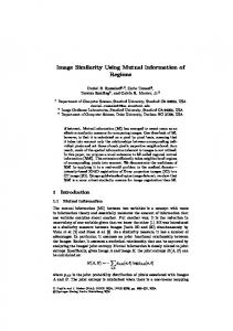
Geometric moment descriptors were computed for three versions of each image filtered by “intensity slicing”, consisting of thresholding the images within three different minimum and maximum intensity ranges (0-50, 50-100, 100-150). The resulting images contained features roughly localized around holes and other structural regions of the object, and segmented from the bright background, as seen in the example of Fig. 1. The input feature vector for the neural network was composed of the moment descriptors computed for all three filtered versions of each image (denoted by the superscripts 50, 100,150), totalling 24 features: f = (ICy e r1 r2 mooS, s ~ ) ~ ~
Reference
Feedforward neural networks were used to learn the direct mapping between feature variations and pose displacements when a robot-mounted camera was moved from a desired reference position. A blackand-white CCD camera mounted on the wrist of a 6-dof industrial robot (GT Productique) was used to acquire a set of 1000 training images of a scene, consisting of an automobile cylinder head on a white table. Images were taken at random poses within
0-50
50-100
100-150
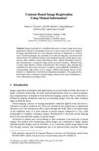
Figure 1 T h e reference image and intensity slices f o r three grey-leuel intervals. For the network trained with KL features, the image projections onto the first 24 eigenvectors of the image set were the inputs. Several of the eigenvectors are shown in Fig. 2. For our work, the SLAM software library [ll]was used to compute the eigenvectors and image projections. The 6 PCI vectors for the image set are shown in
2822
Authorized licensed use limited to: UNIVERSITAT POLITÈCNICA DE CATALUNYA. Downloaded on November 6, 2009 at 05:41 from IEEE Xplore. Restrictions apply.
~
~
4
n
I
3
J
5
7
21
34
The aim, when training a neural network, is to map a subset f of a collection F = { f i ,f i ,...,fm} of prospective input variables (features) to a set y = {yl,y2, ...,yn} of output variables. This is only possible, however, to the extent that some dependence exists between y and f . The more informative the input variables are about the outputs, the lower the network’s final training error will be, assuming that training is efficient in all other respects. Choosing the subset of inputs which is maximally informative about the outputs can therefore help to optimize learning with the available input variables and, with a minimum number of features, reduce training times.
Figure 2: Some eigenvectors of the image set.
Fig. 3. Note that each one has a visible relationship with its corresponding pose component, and that the vector pairs for translational and rotational movements on perpendicular axes are very similar in appearance. Unlike for GM and KL features, the networks trained with PCI features had only 6 inputs.
A useful statistical measure, from Information Theory, for quantifying the dependence between variables is the mutual information. For an input variable f and an output y, which are both assumed to be random variables, the mutual information (MI) is given by
where the summations are computed over the suitably discretized values of f and y. Although probability density estimates, and consequently MI values, are dependent on the number of chosen discretization intervals, in our work the order of selected features was found to be the same for any number between 5 and 20, so 10 intervals were used.
Figure 3: The six P C I vectors of the image set. The final RMS test-set errors for the networks trained with the 3 feature types are shown in Table 1. The values correspond to the lowest errors achieved for 3 training trials of each network. The best results, for all 6 coordinate axes, were clearly obtained for GM features. Error values are somewhat lower for PCI features than for KL features. Table 1: Final RMS test-set errors for neural networks trained with GM, KL and P C I features. Features GM KL PCI
R, R, 0.03 0.05 0.10 0.09
0.20 0.11
R,
T,
T,
0.07 0.22 0.18
0.14 0.41
0.07 0.29 0.25
0.32
T, 0.05 0.29 0.14
Feature selection using mutual information
By measuring the “peakedness” of the joint probability between the variables f and y, the mutual information captures arbitrary (linear and nonlinear) dependencies between them. It is equivalent to the Kullback-Leibler distance, or cross entropy, between the joint distribution and the product of the marginal distributions, and measures the degree to which knowledge provided by the feature vector decreases the uncertainty about the output. Since the features themselves may be dependent on each other, selecting features based only on their individual MI with the outputs can lead to input sets with redundant features which add little to the MI of the set as a whole. The goal is to find a subset of inputs whose MI is maximum with respect to the
2823
Authorized licensed use limited to: UNIVERSITAT POLITÈCNICA DE CATALUNYA. Downloaded on November 6, 2009 at 05:41 from IEEE Xplore. Restrictions apply.
outputs, but minimal with respect to each other. For a given number n of candidate features, the number of possible subsets is 2n and, therefore, computationally expensive to consider when n is large. An alternative is to build a suboptimal set using a heuristic to fulfill these criteria as best as possible. One such method [16] consists of choosing, at each selection step, the candidate feature fi with the smallest euclidean distance from the point of maximum I (f i , y) and minimum I ( fi, f k ) in the 2D space formed by these two variables, where I ( f i ,fk) is the sum of the MI values of the candidate feature f i with the already selected features fk in the set.
ck
the feature set were restricted to increasing minimum threshold values, as shown in Fig. 4. An important observation from this graph is that MI values are much lower overall for the 3 translational components than for the 3 rotational components, resulting in higher RMS errors even for larger feature sets. Rz
ck
-
m
m
201
0.1 18 14 9
The MI selection procedure was applied to a set of all 65 features previously computed for the image set, containing 24 GM, 35 KL, and 6 PCI features. The first 24 features selected for each pose component, in order of decreasing MI, are listed in Table 2.
0'
0.5
I 1
0
01
03
02
04
MI threshold
MI threshold
TX
Table 2: The first 24 MI-selected features from the set of 65 GM, KL and P C I features, in order of decreasing MI.
"0
0.5 MI threshold RY
1
0
01
MI threshold
0.2
0.3
0.4
MI threshold T"
MI threshold
Figure 4: R M S test error us. M I threshold. O n top of each circle the number of features with a n M I value greater than the corresponding threshold is recorded. The RMS error obtained b y training a neural network with only those features is then plotted. Note that the M I scale for the translational axes is half that of the rotational axes, indicating that features are less informative overall for the translational dof 's. The feature sets with the lowest RMS errors are summarized in Table 3.
5 Minimum feature subsets were computed for each pose component by plotting RMS test-set error values versus the number of input features when MI values in
Discussion
The results described in the last two sections can be analyzed in many different ways. Let us first discuss the quantitative benefits resulting from the
2824
Authorized licensed use limited to: UNIVERSITAT POLITÈCNICA DE CATALUNYA. Downloaded on November 6, 2009 at 05:41 from IEEE Xplore. Restrictions apply.
RMS error N features
Rz Rz 0.03 0.05 5 I 10
R,
Tz
Tz
TU
0.08
0.19 24
0.16 24
0.09
16
el5') principal axis for the images of Fig. 1 (e5', seem indeed very relevant and, therefore, it is not surprising that they are among the seven features most highly ranked. The skewness of the projection on also the y axis for the same images (S~o,Sioo,S~50) seem intuitively relevant and, consistently, they are within the 15 most highly ranked. Note also that the image ordering for these two types of features is maintained. The PCI vector for this dof is ranked second, which seems very natural, and more so when one looks at its image-like representation (see Fig. 3). What is more difficult to interpret is the role played by the eigenfeatures. In principle, those with the least concentric symmetry should be selected and, up to what can be seen in Fig. 2 (look at el, in particular), this is consistent with the performed selection.
7
application of the P I criterion.
benefits are also noticeable, for cision is attained with only 7
, in the case of T, and R,,
A similar analysis for the other dof's would be too lengthy to be included in this paper. Let us just mention the clear tendency of geometric moments to appear among the most relevant features, especially in those cases in which a satisfactory precision is reached. Thus, r1 and Z (and 7-2 and 8) prove to be good indicators of variations in R, (and R,, respectively).
although it outperforms
6
t least 10 features have an MI at least 5 of them surpass also ne of the translational dof's leads to similar MI
he error for this dof.
tation of the first
Conclusions
Mutual Information has proven to be a valuable criterion to select image features that are the most variant with camera pose. Its use as a preprocessing step before training a neural network to accomplish visual positioning has lead to a considerable reduction in the number of inputs required to attain a given precision. Besides providing a way to automate the feature selection process, MI permits foreseeing which degrees of freedom will yield larger errors, thus allowing one to look for more informative features before actually training the neural network. In particular, the families of global image features considered in this work provide the most information on R, and the least information on T,, the other dof's falling between them in the following order: R,, R,, Tu and T,. This is in part explained by the image sensitivities to the different dof's. Thus, besides looking for more powerful features to detect variation in the least sensitive dof's, we plan to explore an incremental training procedure. The idea is, for each dof, to use as inputs of the neural network not only the selected image features but also the pose components preceding it in the above order. Then, in operation,
2825
Authorized licensed use limited to: UNIVERSITAT POLITÈCNICA DE CATALUNYA. Downloaded on November 6, 2009 at 05:41 from IEEE Xplore. Restrictions apply.
[5] Faugeras, O., Three Dimensional Computer Vision: A Geometric Viewpoint, MIT Press, Boston, 1993.
R, would be predicted first using only image features, and this predicted value would be used, together with the corresponding selected features, to predict R,, and so on. In this way, the predicted values of five pose components would be used to predict T,.
[6] Fukunaga, K., Statistical Pattern Recognition, 2nd
edition, Academic Press, 1990.
An important feature of the proposed method based on global image descriptors is its general applicability to arbitrary scenes, since the requirement of particular geometric features in the image is avoided. For a chosen scene, the most relevant image features may be selected beforehand using the MI selection procedure and used to train a single neural network, thus avoiding costly trial-and-error with different input sets and reducing training times by keeping the number of inputs to a minimum. Nevertheless, each resulting neural network is specific to the particular scene and lighting conditions for which it is trained, since both the computed features and the feature selection process are dependent on the image characteristics. This system is particularly suited to applications such as visual inspection of components, or repetitive grasping of objects in an industrial environment, where scene and lighting conditions may be kept constant. Notwithstanding, additional preprocessing steps for object segmentation or lighting correction could be applied to allow the use of the method under more varying conditions.
Acknowledgements
[7] Horaud, R. and Dornaika, F., “Hand-eye calibration”, International Journal of Robotics Research, 14(3), pp. 195-210, 1995. [8] Li, W., “Mutual information functions versus correlation functions”, Journal of Statistical Physics, 60(5/6), pp. 328-387, 1990. [9] Mohr, R., Boufama, B. and Brand, P., “Understanding positioning from multiple images”, Artificial Zntelligence, 78(1/2), pp. 213-328, 1995. [lo] Nayar, S., Nene, S. and Murase, H., “Subspace
Methods for Robot Vision”, IEEE Transactions on Robotics and Automation, (pending publication). [ll] Nene, S., Nayar, S. and Murase, H., “SLAM: Software
Library for Appearance Matching”, Technical Report CUCS-019-94, Department of Computer Science, Columbia University, Columbia, NY, 1994. [12] Prokop, R. and Reeves, A., “A survey of momentbased techniques for unoccluded object representation and recognition”, Graphical Models and Image Processing, 54(5), pp. 438-460, 1992. [13] Sipe, M., Casasent, D. and Neiberg, L., “Feature Space Trajectory Representation for Active Vision”, Proc. SPIE, April 1997.
This research has been partially supported by the research grant CICYT TAP97-1209 of the Spanish Science and Technology Council.
[14] Sturm, P., “Critical motion sequences for monocular self-calibration and uncalibrated euclidean reconstruction”, Proc. IEEE Conf. on Computer Vision and Pattern Recognition, Puerto Rico, pp. 1100-1105, June 1997.
References
[15] Wells, G., Venaille, C. and Torras, C., “Vision-based robot positioning using neural networks” , Image and Vision Computing, 14, pp. 715-732, 1996.
[l] Bien, Z., Jang, W. and Park, J., “Characterization
and use of feature-Jacobian matrix for visual servoing”, in Visual Servoing, edited by K. Hashimoto, pp. 317-363, World Scientific, Singapore, 1993.
[16] Zheng, G. and Billings, S., “Radial basis funcion network configuration using mutual information and the orthogonal least squares algorithm”, Neural Networks, 9(9), pp. 1619-1637, 1996.
[2] Cibas, T., Fogelman, F., Gallinari, P. and Raudys, S., “Variable selection with neural networks”,
Neurowmputing, Vol. 12, pp. 223-248, 1996. [3] Corke, P., “Visual Control of Robot Manipulators - A Review”, in Visual Servoing, edited by K. Hashimoto, pp. 1-31, World Scientific, Singapore, 1993. [4] Espiau, B., Chaumette, F. and Rives, P., “A New Approach to Visual Servoing in Robotics”, IEEE Transactions on Robotics and Automation, 1992.
2826
Authorized licensed use limited to: UNIVERSITAT POLITÈCNICA DE CATALUNYA. Downloaded on November 6, 2009 at 05:41 from IEEE Xplore. Restrictions apply.