Robot Tasks Sequence Planning using Petri Nets Jan Rosell
Norberto Mu˜ noz
Antonio Gambin
Institut d’Organitzaci´ o i Control de Sistemes Industrials Diagonal 647, 08028 Barcelona, SPAIN
[email protected]
[email protected]
Abstract The automatic programming of robots to assemble products must cope with assembly planning and task planning problems. These problems are not independent, since an assembly operation may be performed by a different robot task depending on the previous assembly operations performed. Therefore, the cost of assembly operations vary depending on the assembly sequence. This paper deals with the problem of finding the optimum sequence of robot tasks taking into account this variable cost of assembly operations. The proposed approach can cope with products with AND/OR/XOR relations and uses Petri nets as a modelling methodology. The search of a near-optimum sequence of robot tasks is done with an heuristic search of the reachability tree of the Petri net.
SADIEL S.A. Barcelona, SPAIN
[email protected]
a different robot task depending on the previous assembly operations performed. Therefore, the cost of executing an assembly operation depends on the assembly sequence. Petri nets is a modelling formalism that has been used in both assembly planning and task planning. The use of the same modelling technique can cope with the conflicts and interactions between assembly planning and task planning, and be an aid towards the obtention of an autonomous robotic assembly system [5]. This paper copes with the problem of finding the minimum-cost sequence of robot tasks to perform a sequence of assembly operations that enables to assemble a product, using Petri nets as modelling methodology.
1.2
1
∗
Petri Nets Formalism
Introduction
1.1
Framework and problem statement
The aim of an autonomous robotic assembly system is to execute an assembly task from a high level description of the product to be assembled, which involves problems related to both assembly planning and task planning [1]. Assembly planning is generally associated with sequence planning, i.e. the determination of a (feasible and optimal) sequence of parts to be mated in order to assemble a product. Task planning deals with the translation of an assembly plan into the robot operations that may allow the successful execution of the task. The performance of each step in an assembly sequence can be done by different robot tasks depending on the type of operation, the pair of subassemblies involved, their symbolic spatial relations, the local depart space, or the tool used for the task [2, 3, 4]. Moreover, a given assembly operation may be performed by ∗ This
work was partially supported by the CICYT projects DPI2002-03540 and DPI2001-2202
Petri nets is a formalism that allows to model systems involving concurrency, resource sharing, synchronization and conflict, and allow to validate the correctness of the system by analyzing the qualitative properties of the net modelling the system. A Petri net model of a discrete-event dynamic system is composed of a net structure with two disjoint sets of objects: places (represented as circles) that are the support of the state variables, and transitions (represented as bars) that represent the events. Places and transitions are connected by arcs following a weighted flow relation. The dynamics of the net structure is coded by a marking (an assignment of tokens to each place) and the marking evolution rule known as token game. Formally, a Petri net is defined as a five tuple [6]: N =< P, T, P re, P ost, M0 >
(1)
where P is a finite non-empty set of places, T is a finite non-empty set of transitions, P re is the pre-incidence function P × T → ℵ+ , P ost is the post-incidence func-
tion T × P → ℵ+ , and M0 is the initial marking (the initial assignment of tokens to each place). Pre and post-incidence functions can be represented by means of matrices of |P | rows and |T | columns. If the net has no self-loops then the net is fully characterized by a single incidence matrix C = P ost − P re, such that if there is an arc with weight k ∈ ℵ+ from ti to pj then C[pj ][ti ] = k, and if there is an arc with weight k ∈ ℵ+ from pj to ti then C[pj ][ti ] = −k. One of the methods to analyze the dynamics features of a Petri net is by means of the reachability tree, which is a tree whose nodes are the markings that are reachable from the initial marking M0 , the arcs being labelled by the transition to be fired to change from and marking to the next.
1.3
Assembly planning and task planning using Petri nets
One of the main works in assembly planning using Petri nets is that of Cao and Sanderson [7]. These authors describe an extension of AND/OR graphs from a tree to a net structure, and present a mapping from the AND/OR net representation of an assembly to a Petri net, in order to ease the analysis of the qualitative properties of the system. The obtained Petri net is demonstrated to be safe, live and reversible. The searching of assembly sequences is done from the Petri net by analyzing the corresponding reachability tree. In order to cope with complex AND/OR relationships, that cannot be modelled by means of AND/OR graphs, Moore et al. [8] propose an algorithm, based on the assembly by disassembly concept, that generates a disassembly Petri net from a geometricallybased disassembly precedence matrix obtained from a CAD representation of the product. Their proposed algorithm guarantees that, with a small number of restrictions, the obtained disassembly Petri Net is live, bounded and reversible. Near-optimal disassembly sequences are obtained from the corresponding reachability tree using an heuristic search approach. Task planning usually requires the performance of motions in contact, which rely on a graph representation of the contact space. Assuming that the contact state graph of a given assembly task is known, McCarragher [9] models it by means of Petri nets using both state places and control places. State places represent basic contacts of the assembly (the simultaneous marking of state places representing multi contact situation), and transitions represent the gaining or losing of a basic contact. Control places represent conditions of external inputs that enable transition to occur and are connected to each transition by an inhibitor arc. A
trajectory planer defines a performance measure and finds a path in the Petri net that maximizes it.
2
Proposed solution
The proposed solution to the problem stated in Section 1 is based on the assembly by disassembly concept. First, a precedence matrix (M) is obtained from the CAD model of the part to be assembled and the use of a geometric tool that solves the assembly partitioning problem [10]. Then, using an extension of the approach of Moore et al. [8], a disassembly Petri Net is obtained from M, where each transition represents the disassembly of a given part (a variable cost is assigned to the firing of each transition, which depends on the previous firings). Finally, a near-optimum disassembly sequence is obtained by doing an heuristic exploration of the reachability tree of the Petri Net [11]. Then, the assembly sequence is the reverse one. In this paper, only 2D assembly tasks with polygonal parts will be considered.
2.1
Precedence matrix
Let the product to be assembled be composed of N parts, each one identified by a numeric label ranging from 1 to N . Then, the disassembly precedence matrix M is a N ×N matrix that describes the precedence relationships between parts, i.e. determines which parts must be removed before being able to remove another one. The information for a given part i is codified in column i as follows: • If parts j and k are AND precedents to part i, then M[j][i] and M[k][i] are set to the same positive integer value, and all the other rows are set to zero. • If parts j and k are OR (XOR) precedents to part i, then M[j][i] and M[k][i] are set to different positive (negative) integer values, and all the other rows are set to zero. This section presents an algorithm to automatically generate the precedence matrix. It makes use of a geometric tool that checks if there exists an infinitesimal motion that rigidly removes a polyhedral part from the assembled product [10]. The algorithm studies the arrangement of hyperplanes tangent to the C-surfaces associated with the effective contacts, at the given configuration of the polyhedron to be removed. The free convex cones of maximum dimension of the hyperplanes arrangement define the separating motions.
These free convex cones are determined by the simple evaluation of boolean expressions. The following variables and functions are used in the algorithm to compute M. • P : Product to be assembled, composed of N parts. It is a list of indices (ranging from 1 to N ) representing its parts • A[i]: List of the indices of the parts not yet disassembled at step i of the algorithm. A[0] contains all the parts of the assembled product, with indices ranging from 1 to N • B: List of the indices of the parts already disassembled
Precedence Matrix Generation(P ) A[0] = P M = zero matrix N × N FOR i = 1 TO card(A[0]) DO
e ← element(A[0], i) IF disassembly(e, ∅, P , M) = TRUE THEN
insert({e}, B) ELSE insert({e}, A[1]) END IF END FOR DO
T =∅
• Bp : List of groups of p elements of B. Each group is represented as a list
FOR p = 1 TO card(B)
Bp =combine(B,p)
• T : Auxiliary list of the indices of parts that can be disassembled
FOR i = 1 TO card(A[p]) DO
e ← element(A[p], i)
Let the parameters X and Y be two lists of parts, then the following functions are used:
FOR k = 1 TO card(Bp ) DO
• card(X): returns the number of elements of X
IF disassembly(e,Bp [k],P ,M) = TRUE THEN
• element(X, j): returns the jth element of X
M[j][e] = label(Bp [k]) ∀j ∈ Bp [k]
• insert(X,Y ): inserts X at the end of Y
insert({e}, T )
• subs(X,Y ): eliminates from X the elements of Y
END IF
• empty(X): returns TRUE if list X is empty, and FALSE otherwise
END FOR END FOR
• combine(X,k): returns a list with all the groups of k elements of X
A[p + 1] = subs(A[p], T ) END FOR
• label(X): returns a unique label to X. Labels are positive integers • disassembly(j,X, Y , M): returns TRUE if part j can be disassembled from the assembly represented by Y iff parts of X and their precedents, as indicated in M, have been previously disassembled, and FALSE otherwise • verifyXOR(M): For each OR precedence relationship in M, applies the disassembly function to verify if the disassembly operation can be performed when all the OR precedents are previously removed. If it is not the case, there exists a XOR relationship and then the corresponding labels in M are negated. Finally, the algorithm to generate the precedence matrix is the following.
B = insert(T, B) WHILE NOT empty(A[p + 1])
verifyXOR(M) END
2.2
Neighboring contact matrices
The edge-edge contact between parts are considered. Two parts form a contact pair in the x direction if the projection of any of the contact edges onto the x axis is larger than the projection onto the y axis. Otherwise it is considered a contact pair in the y direction. It is assumed that two contact matrices, Kx and Ky , can be obtained from the CAD model of the product to be assembled. The dimension of these matrices are 2 × nx and 2 × ny , respectively, being nx and ny the number of contact pairs in the x and y directions.
PSfrag replacements
a)
b) 1 2
1
3
4
a)
3 4
5
2
c)
1 PSfrag replacements
6
Petri net model
Let: • M[i][·] and M[·][j] represent, respectively row i and column j of M. • C be the incidence matrix of the Petri net. • the set of transitions be composed of N + 2 transitions, such that ti represents the disassembly of part i, and t(N +1) and t(N +2) represent the starting and the completion of the disassembly, respectively. • the initial set of places be composed of N + 2 places, such that pi represents the preconditions to removing part i, p(N +1) represents the beginning (i.e. the assembled product) and p(N +2) represents the preconditions for the completion of the disassembly. The set of places is enlarged when modelling OR or XOR precedence relationships. The new places are labelled as pk with k starting at (N + 3). • Li be a label associated to transition ti . From the disassembly precedence matrix obtained in Section 2.1, a Petri net is generated following the approach of Moore et al. [8] according to the following considerations: • When part j has no precedents then M[·][j] contains only zeros. In this case, C[pj ][t(N +1) ] = 1 and C[pj ][tj ] = −1. • When the removal of part i is no precedent to the removal of any other part (only a precondition to the complete disassembly) then M[i][·] contains only zeros. In this case, C[p(N +2) ][ti ] = 1.
1 2
2 d)
c) 1 x
Matrix Kx (Ky ) contains in each column the indices of the parts that form a contact pair in the x (y) direction. As an example, the neighbor contact matrices of Figure 1a are: ¶ ¶ µ µ 1 2 3 1 2 (2) Ky = Kx = 4 4 4 2 3
1
2 y
Figure 1: Simple products to be assembled.
2.3
b)
2
1 2
Figure 2: Robot tasks, in the x-direction, to assemble e) manipulated part 1 with fixed part 2: a) Put-Down b) Alignment c) Peg-into-Hole d) 1.5-Peg-into-Hole e) 2-Peg-into-Hole.
• When the removal of R parts ki with i ∈ 1 . . . R are AND precedent to the removal of part j, then M[ki ][j] = Lki ∀i ∈ 1 . . . R with Lki = Lkj ∀i, j. In this case, C[pj ][tki ] = 1 ∀i ∈ 1 . . . R, and C[pj ][tj ] = −R. • When the removal of any part ki with i ∈ 1 . . . R is precedent to the removal of part j, there is an OR precedence relationship. Then, M[ki ][j] = Lki ∀i ∈ 1 . . . R with Lki 6= Lkj ∀i 6= j. In this case, a new place poj is created, and C[poj ][tj ] = −1, C[poj ][tki ] = 1 ∀ ki with i ∈ 1 . . . R, C[poj ][t(N +2) ] = −R + 1, and C[pj ][tj ] = −1, and C[pj ][t(N +1) ] = 1. • When the removal of any part ki with i ∈ 1 . . . R (but not all of them) is precedent to the removal of part j, there is an XOR precedence relationship. Then M[ki ][j] = −Lki ∀i ∈ 1 . . . R with Lki 6= Lkj ∀i 6= j. In this case, two new places pcj and pxj are created, and C[pcj ][tki ] = −1 ∀ ki with i ∈ 1 . . . R, C[pcj ][t(N +1) ] = 1, C[pcj ][tj ] = R − 1, C[pxj ][tj ] = −1, C[pxj ][tki ] = 1 ∀ ki with i ∈ 1 . . . R, C[pxj ][t(N +2) ] = −R + 1, C[pj ][tj ] = −1, and C[pj ][t(N +1) ] = 1. • C[p(N +1) ][t(N +1) ] = −1, C[p(N +2) ][t(N +2) ] = −1 and C[p(N +1) ][t(N +2) ] = −1. The resulting Petri net is demonstrated to be safe, live and reversible.
2.4
Robot tasks encoding
The following robot tasks, associated to either the x or y direction, are considered [2] (Figure 2): PutDown, Alignment, Peg-into-hole, and n-Peg-into-hole. The kind of robot task needed is determined using the information of the contact matrices. Let consider
first Kx . If the part is not in Kx , then it has no constraints in the x direction and it is considered as an Alignment (in this case, no guarded motion can l be performed in the x direction to fix the part in its final position). If the part is exclusively in one column n=2 of Kx , then there is a one-side constraint and the PSfrag task replacements is considered a Put-Down in this direction. If the part is in both columns of Kx , then it is a Peg-into-hole, Figure 3: Exploration of the reachability tree. e.g. if it appears twice in each column it is a 2-Peginto-hole, if it appears once in each column it is a Peginto-hole, and if it appears once in a column and twice in the other then it is a 1.5-Peg-into-hole. The same is associated to the robot tasks are dynamically encoded done with Ky . as a cost function that can be evaluated at each markThe following qualitative costs are associated to the ing of the Petri net. At a given marking, the parts of robot tasks according to the difficulty in their executhe product that have been already disassembled are tion. The cost of an operation is considered as the known by looking to the firing sequence that lead to sum of the costs in each direction. that marking. Using this knowledge and the contact matrix described in Section 2.2, it is possible to deRobot Task Cost termine which robot task from those described in SecPut Down 1 tion 2.4 is required to perform the action described by Alignment 2 the enabled transition, and assign to that transition Peg-into-hole 3 the corresponding cost of the robot action. n-Peg-into-hole 3n As an example, consider the costs in the x direction of the assembly task presented in Figure 1a. If the assembly sequence is 4 − 1 − 2 − 3 the operation of assembling part 2 can be performed by a Put-Down robot task. Nevertheless, if the assembly sequence is 4 − 1 − 3 − 2, then the operation of assembling part 2 must be performed by a Peg-into-hole robot task, which results in a more expensive assembly sequence.
2.5
Optimization
The difficulty in the analysis of Petri nets by means of the reachability tree relies in the size of such tree. In order to offer a suitable solution of production planning problems following this approach, a programming tool capable of making a partial exploration of the reachability tree of timed Petri nets by means of an heuristic algorithms was developed by Gambin et al. [11]. The reachability tree exploration is done by iteratively decomposing it into a set of n subtrees of constant depth l, i.e. each subtree is exhaustively explored from its root to a level l and then the n markings with a lowest cost are selected as roots for the next set of subtrees (Figure 3). The values n and l are specified by the user. This partial exploration of the reachability tree ends with a near-optimum sequence of transition firings. This tool has been adapted in order to be able to assign a variable cost to each transition. The costs
3
An example
Let us consider the task of assembling the product shown in Figure 1b. In this task there are AND and XOR precedence relationships. The precedence and contact matrices of this task are the following:
0 0 0 M= 0 0 0
0 0 0 0 0 0
1 1 0 0 0 0
0 0 0 0 −2 −3
4 0 0 0 0 0
0 5 0 0 0 0
(3)
Kx =
µ
5 5 5 5 1 4 3 2 6 3 1 3 2 3 4 6 1 5 6 6 6 2 1 3 2 3
Ky =
µ
1 2 3 3 3 4 5 4 6 5 6 4 5 6 5 4 6 4
(4) (5)
From M a Petri net with the following incidence matrix is obtained. There are 8 transitions: t1 to t6 correspond to the six parts of the assembly and t7 and t8 are the initial and the final transitions, respectively. There are 10 places: p1 to p6 correspond to the six parts of the assembly, p7 and p8 are the initial and final places, and p9 and p10 the additional places for the XOR precedence relationship.
t1 p1 −1 p2 0 p3 1 p4 0 C = p5 1 p6 0 p7 0 p8 0 p9 0 p10 0
t2 0 −1 1 0 0 1 0 0 0 0
t3 0 0 −2 0 0 0 0 1 0 0
t4 0 0 0 −1 0 0 0 1 1 −1
t5 0 0 0 0 −1 0 0 0 −1 1
t6 0 0 0 0 0 −1 0 0 −1 1
t7 1 1 0 1 0 0 −1 0 1 0
t8 0 0 0 0 0 0 1 −1 0 −1
(6)
References
The cost function to explore the reachability tree uses the neighboring contact matrices Kx and Ky of equation (5). The following results are obtained, using n = 2 and l = 5 as exploration parameters: • Solution disassembly sequence: 1-2-3-5-4-6 • Robot tasks used: Part 1 2 3 5 4 6 TOTAL
Robot Task y 2-Peg-into-hole 2-Peg-into-hole Peg-into-hole Peg-into-hole Peg-into-hole Alignment
Robot Task x Put-Down Put-Down Put-Down Put-Down Put-Down Alignment
Cost 6+1 6+1 3+1 3+1 3+1 2+2 30
With the complete exploration of the reachability tree, the same optimum sequence was obtained in few seconds. Obviously, for this simple assembly task this is not a constraint but for a real assembly task with more parts, the exhaustive exploration could not be affordable.
4
dence matrix. Each transition of the Petri net represents the disassembly of a given part, and a variable cost is assigned to its firing, which depends on the previous firings performed, i.e. on the previous operations performed. The search of a near-optimum sequence of robot tasks is done with an heuristic search of the reachability tree of the Petri net.
Summary
The cost of assembly operations vary as a function of the assembly sequence, since they may be performed by different robot tasks depending on the previous assembly operations performed. Taking into account this fact, the paper proposes a solution for the problem of finding a near-optimum sequence of robot tasks. The proposed approach, based on the assembly by disassembly concept, can cope with products with AND/OR/XOR relations and that require arbitrary infinitesimal motions to rigidly remove a part from the assembly. Petri nets are used as a modelling methodology, following the approach of Moore et al. [8] to automatically generate them from the disassembly prece-
[1] S. Gottschlich, C. Ramos, and D. Lyon, “Assembly and task planning taxonomy,” IEEE Robotics and Automation Magazine, pp. 4–12, September 1994. [2] H. Moseman and F. M. Whal, “Automatic decomposition of planned assembly sequences into skill primitives,” IEEE Trans. on Robotics and Automation, vol. 17, no. 5, pp. 709 –718, 2001. [3] W. H. Quian and E. Pagello, “On the scenario and heuristics of disassemblies,” in Proceedings of the IEE, pp. 264–271, 1994. [4] S. K. Lee and F. C. Wang, “Physical reasoning of interconnection for efficient assembly planning,” in Proc. of the IEEE Conf. on Robotics and Automation, pp. 307–313, 1993. [5] J. Rosell, “Assembly and task planning using Petri nets: A survey and a roadmap towards autonomous robotic assembly systems,” technical report IOC-DTP-2002-13, Univ. Polit`ecnica de Catalunya, 2002. [6] M. Silva, Practice of Petri Nets in Manufacturing, ch. Introducing Petri nets, pp. 1–62. Chapman & Hall, 1993. [7] T. Cao and A. C. Sanderson, “AND/OR Net representation for robotic task sequence planning,” IEEE Trans. Syst., Man and Cybernetics - Part C: Applications and Reviews, vol. 28, pp. 104–218, May 1998. [8] K. E. Moore, A. G¨ ungor, and S. M. Gupta, “Petri net approach to disassembly process planning for products with complex AND/OR precedence relationships,” European Journal of Operational Research, vol. 135, pp. 428–435, 2001. [9] B. J. McCarragher, “Petri net modelling for robotic assembly and trajectory planning,” IEEE Trans. on Industrial Electronics, vol. 41, pp. 631–640, Dec. 1994. [10] E. Staffetti, L. Ros, and F. Thomas, “A simple characterization of the infinitesimal motions separating general polyhedra in contact,” in Proc. of the IEEE Int. Conf. on Robotics and Automation, vol. 1, pp. 571 –577, 1999. [11] A. J. Gambin, M. A. Piera, and D. Riera, “A Petri nets based object oriented tool for the scheduling of stochastic flexible manufacturing systems,” in Proc. of the 7th IEEE Int, Conf. on Emerging Technologies and Factory Automation, vol. 2, pp. 1091 –1098, 1999.