ARTICLE International Journal of Advanced Robotic Systems
Robust Adaptive Neural Sliding Mode Approach for Tracking Control of a MEMS Triaxial Gyroscope Regular Paper
Juntao Fei*, Hongfei Ding, Shixi Hou, Shitao Wang and Mingyuan Xin Jiangsu Key Laboratory of Power Transmission and Distribution Equipment Technology College of Computer and Information, Hohai University, China * Corresponding author E-mail:
[email protected] Received 15 Mar 2012; Accepted 10 Apr 2012 DOI: 10.5772/50915 © 2012 Fei et al.; licensee InTech. This is an open access article distributed under the terms of the Creative Commons Attribution License (http://creativecommons.org/licenses/by/3.0), which permits unrestricted use, distribution, and reproduction in any medium, provided the original work is properly cited.
Abstract In this paper, a neural network adaptive sliding mode control is proposed for an MEMS triaxial gyroscope with unknown system nonlinearities. An input‐output linearization technique is incorporated into the neural adaptive tracking control to cancel the nonlinearities, and the neural network whose parameters are updated from the Lyapunov approach is used to perform the linearization control law. The sliding mode control is utilized to compensate the neural network’s approximation errors. The stability of the closed‐loop system can be guaranteed with the proposed adaptive neural sliding mode control. Numerical simulations are investigated to verify the effectiveness of the proposed adaptive neural sliding mode control scheme.
Keywords Neural Network, Sliding Mode Control, Robust Control, Adaptive Control, Lyapunov’s Direct Method
1. Introduction
A gyroscope is a commonly used sensor for measuring angular velocity in many areas of application, such as www.intechopen.com
navigation, homing and control stabilization. The performance of the MEMS gyroscope is deteriorated by the effects of time‐varying parameters as well as noise sources, quadrature errors, parameter variations and external disturbances, which generate a frequency of oscillation mismatch between the two vibrating axes.
It is necessary to control the MEMS gyroscope using advanced control approaches, such as adaptive control, sliding mode control and intelligent control. In the last few years, various control approaches have been presented to control the MEMS gyroscope. Increasing attention has been given to the tracking control of the MEMS gyroscope. Batur et al. [1] developed a sliding mode control for a MEMS gyroscope system. Sun et al. [3] derived a phase‐domain design approach to study the mode‐matched control of a gyroscope. Park et al. [4] presented an adaptive controller of a MEMS gyroscope which drives both axes of vibration and controls the entire operation of the gyroscope. John et al. [5] proposed a novel concept for an adaptively controlled triaxial angular velocity sensor device. Fei [6‐7] derived an adaptive sliding mode controller and a robust adaptive controller for a MEMS vibrating gyroscope.
Int J Adv Sy, 2012, 9, 24:2012 Juntao Fei, Hongfei Ding, Shixi Hou,Robotic Shitao Wang andVol. Mingyuan Xin: Robust Adaptive Neural Sliding Mode Approach for Tracking Control of a MEMS Triaxial Gyroscope
1
Model reference adaptive control (MRAC) methods have been widely applied to robotic systems. Detailed physical descriptions regarding to the robotic system using MRAC have been discussed [8‐10]. Recently, much research has been done to apply intelligent control approaches such as neural networks and fuzzy controls that do not require mathematical models and have the ability to approximate nonlinear systems. Therefore, intelligent control approaches have been applied to represent complex plants and to construct advanced controllers. Wang [11] proposed a universal approximation theorem and demonstrated that an arbitrary function of a certain set of functions can be approximated with arbitrary accuracy using a fuzzy system on a compact domain. Adaptive fuzzy sliding mode control schemes have been developed for robotic manipulators [12‐13]. A neural network has the ability to approximate any nonlinear function over a compact input space. Therefore, a neural network’s learning ability to approximate arbitrary nonlinear functions makes it a useful tool for adaptive application. Tracking controls using neural networks for nonlinear dynamic systems have become a promising research topic. Lewis et al. [14] developed neural network approaches for robotic manipulators. Horng [15] proposed a neural adaptive tracking control for a DC motor with unknown system nonlinearities where neural network approximation errors are compensated for by using the sliding mode scheme. Yu et al. [16] presented a direct adaptive neural control with a sliding mode method for a class of uncertain switched nonlinear systems. Lin et al. [17] used a neural network‐based robust nonlinear control for a magnetic levitation system. Neural network sliding mode control approaches have been developed for robotic manipulators [18‐19].
This paper focuses on the design of an adaptive neural sliding mode control based on input‐output linearization. A robust adaptive neural sliding mode tracking control approach is presented for a MEMS gyroscope. By employing radial‐basis‐function neural networks to account for system uncertainties, the proposed scheme is developed by combining feedback linearization techniques and neural learning properties. The control scheme integrates the theory of sliding mode control and the nonlinear mapping of a neural network. A RBF neural network is used to adaptively learn the linear control component. The key property of this scheme is that the weights of the neural network are estimated adaptively and the velocity and position of the MEMS gyroscope are forced to follow any arbitrary trajectory.
The paper is organized as follows. In section 2, the dynamics of a triaxial MEMS gyroscope are introduced. In section 3, a feedback linearization procedure is described and a sliding mode control using a feedback linearization approach is proposed to guarantee the asymptotic stability of the closed loop system. In section 4, an adaptive neural network sliding mode control is developed. The simulation results are presented in 2
Int J Adv Robotic Sy, 2012, Vol. 9, 24:2012
section 5 to verify the effectiveness of the proposed control. Conclusions are provided in section 6.
2. Description of a motion equation of a mems triaxial gyroscope
Assume that the gyroscope is moving with a constant linear speed with respect to an inertial system of reference; that the gyroscope is rotating at a constant angular velocity; that the centrifugal forces are assumed negligible; that the gyroscope undergoes rotations along the x , y and z axis. The nonlinear motion equations of such a triaxial gyroscope can be derived as:
mx dxx x dxy y dxz z kxx x kxy y kxz z m( 2y 2z )x mx y y mx z z ux 2mz y 2my z
my d xy x d yy y d yz z kxy x k yy y k yz z m( 2x 2z )y m y x x m y z z u y 2mz x 2mx z mz d xz x d yz y d zz z kxz x k yz y kzz z m( 2x 2y )z mx z x m y z y uz 2m y x 2mx y
(1)
where m is the mass of proof mass fabrication imperfections contributing mainly to the asymmetric spring terms k xy , k xz and k yz and asymmetric damping terms d xy , d yz and d xz ; k xx , k yy and k zz are spring terms; d xx , d yy and d zz are damping terms; x , y and z are angular velocities; u x , u y and u z are the control forces in the x , y and z directions respectively.
Dividing the equation by the reference mass, and because
of the non‐dimensional time t w0 t , then dividing 2
both sides of the equation by the reference frequency w0 and the reference length q0 and rewriting the dynamics in vector forms result in:
K q q q D q u q (2) a2 b2 2 2 q0 mw0 q0 mw0 q0 mw0 q0 mw0 q0 w0 q0
where
0 z y x u x x , 0 q y , u uy , z y x 0 z u z
d xx D d xy d xz
d xy d yy d yz
k xx d xz , d yz K a k xy k xz d zz
2y 2z x y b 2x 2z y x 2x 2y x z
k xz k yz , k zz
k xy k yy k yz
x z yz y z
www.intechopen.com
Rewriting (4) as:
We define the new parameters as follows:
q
uy
wx
wxy
q D ux , D , , ux , 2 q0 mw0 w0 mw0 q0 uy 2
mw0 q0 k xx mw0
k xy mw0
2
2
, uz , wy
uz
2
mw0 q0
k yy mw0
, w yz
2
k yz mw0
2
k zz mw0
, wxz
2
k xz mw0
Rewriting (5) as:
,
2
q ( D 2)q kb q b q u d1 (6)
.
wy
2
w yz
d1 represents the lumped model uncertainties
d1 d Dq Kb q
q Dq kb q b q u 2q (3) w xy
and external disturbances which are given by
The final form of the non‐dimensional equation of motion can be obtained by ignoring the superscript:
wx 2 where K b w xy w xz
where
,
, wz
q ( D 2 )q K b q u d1 (5)
define:
f (q, q , t ) ( D 2)q kb q b q d1 (7)
where
f q, q , t is an unknown nonlinear function.
Therefore, (6) becomes
w xz w yz . 2 wz
q f ( q, q , t ) u (8) The control target for the MEMS gyroscope is to maintain the proof mass so as to oscillate in the x , y and z
3. Sliding mode control directions at a given frequency and amplitude: The sliding mode control is a robust control technique xm A1 sin(1t ), ym A2 sin(2t ), and which has many attractive features, such as robustness to parameter variations and insensitivity to external zm A3 sin(3t ) . Then, the reference model can be disturbance. The sliding mode controller is composed of defined as: an equivalent control part that describes the behaviour of the system when the trajectories stay over the sliding qm K m qm 0 (9) manifold and a variable structure control part that enforces the trajectories to reach the sliding manifold and T where qm xm ym zm , K m diag{12 , 2 2 , 3 2 } . prevent them leaving the sliding manifold. The sliding mode has some limitations, such as chattering and high frequency oscillation in practical applications. Define the tracking error and sliding surface as follows: In this section, a novel sliding mode controller can be e q qm (10) designed for the MEMS gyroscope with unknown system nonlinearities so as to guarantee the asymptotic stability s ( q, q , t ) Ce e (11) of the closed loop system. According to feedback linearization technique, the sliding Consider the dynamics with parametric uncertainties and mode controller can be designed as: external disturbance as: f ( q , q , t ) q ( D 2 D )q ( K b K b )q b q u d (4) u R where D is the unknown parameter uncertainty of the matrix, D 2 , K b is the unknown parameter uncertainty of the matrix K b , and d is the external disturbance of the system .
www.intechopen.com
q, q , t sgn( s ) f (q, q , t ) (12) qm Ce sgn( s ) f ( q, q , t )
where R q, q , t sgn( s ), 0 and
( q, q , t ) qm Ce . Juntao Fei, Hongfei Ding, Shixi Hou, Shitao Wang and Mingyuan Xin: Robust Adaptive Neural Sliding Mode Approach for Tracking Control of a MEMS Triaxial Gyroscope
3
Define the Lyapunov function:
V
1 T s s (13) 2
The derivative of the Lyapunov function with respect to time becomes:
V sT s sT (e Ce)
sT (q qm Ce) sT f (q, q , t ) u qm Ce
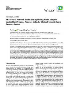
greatly accelerating the learning speed and avoiding the local minimum problem. The block diagram of the sliding mode control using the RBF neural network is shown in Fig. 2.
h1
q
x1
q
(14)
h2 h3
x2
2 3 4
1
fˆ
h4
Substituting (12) into (14) yields:
Figure 1. The structure of the RBF network
V sT sgn( s) s 0 (15)
V becomes negative and semi‐definite, implying that the
trajectory reaches the sliding surface in a finite time and remains on the sliding surface. It can be shown that s( t ) will asymptotically converge on zero, lim s (t ) 0 ,
fˆ
qm
t
lim e(t ) 0 .
f q, q , t in (13) is an unknown function,
therefore the controller (18) cannot be implemented directly and it is necessary to replace f ( q, q , t ) by the RBF neural network output
fˆ (q, q , t ) to realize the
adaptive neural sliding mode control. The structure of the RBF neural network is a three‐layer feedforward network shown as in Fig. 1. The block diagram of the RBF network is shown as follows: the input of the neural network is and
x q, q
T
,,
h1 , h2 , h3
the RBF network is the unknown nonlinear function
fˆ .
The input layer is the set of source nodes. The second layer is a hidden layer of a high dimension. The output layer gives the response of the network to the activation patterns applied to the input layer. The input into an RBF network is nonlinear while the output is linear, thus Int J Adv Robotic Sy, 2012, Vol. 9, 24:2012
qm
Figure 2. Block Diagram of the sliding mode control using the RBF network
The estimate of
fˆ is:
fˆ T x (16)
where x q network, and
q is the input of the RBF neural
T are weights of the RBF neural network
( x) is a Gaussian function:
i ( x) exp(
x mi
2
i2
) , i 1, 2, 3 (17)
mi is the centre of the number i neurons, i is width of number i neurons.
where
Assumption. There exists a coefficient’s weight
that
such
fˆ approximates the continuous function f
an accuracy
h4 are Gaussian functions, 1 , 2 , 3 and 4
are the weights of the RBF neural network, the output of
4
q
t
4. Adaptive Neural Sliding mode controller We will address the design of an adaptive RBF network based sliding mode control problem. Because of the great advantages of neural networks in dealing with nonlinear systems, an adaptive neural sliding mode controller is designed and its stability is analysed in this section. Adaptive neural network sliding mode control is adopted to facilitate the adaptive tracking control of the MEMS gyroscope. In the practical application of the MEMS gyroscope,
q, q
u
, that is:
with
max fˆ (q, q , ) f (q, q ) (18)
Suppose t is the estimate of
at time t , then the
control law becomes:
u (t ) R fˆ (q, q , t ) (19)
www.intechopen.com
where:
Substituting (28) into (27) and choosing
fˆ (q, q , t ) t h (20)
The derivative of the sliding surface is:
u R f (q, q , t )
yields:
as in (18) into (27)
s f (q, q , t ) R fˆ (q, q , t ) (q, q , t )
[ f ( q, q , t ) fˆ ( q, q , t )] ( q, q , t ) sgn( s ) ( q, q , t ) [ fˆ ( q, q , ) fˆ ( q, q , t )] [ f ( q, q , t ) fˆ ( q, q , )] sgn( s ) fˆ ( q, q , ) fˆ ( q, q , ) t sgn( s )
V becomes negative and semi‐definite, implying that the
trajectory reaches the sliding surface in a finite time and
remains on the sliding surface. V is negative and definite which implies that
V , s,
as
t
0
s dt
1
(t )
[V (0) V (t )] . Since V ( 0 ) is
bounded and V ( t ) is non‐increasing and bounded, it can be concluded that lim
(t ) t (23)
Then the sliding dynamics of (22) becomes:
s [ T J (t )] sgn( s) (24) where:
t
0
s dt is bounded. Since
0
according
to
the
Barbalat
fˆ ( q, q , ) 2 , (t ) ( ) ( ) (25) J t
Define a Lyapunov function:
1 T 1 s s (t )T (t ) (26) 2 2
The derivative of the Lyapunov function with respect to time becomes: V sT s (t )T (t ) s sT [ (t )T J (t )] (t )T (t )
s sT (t )] [ sT (t )T J (t )T (t )]
(t ) Js (28)
s( t ) will
lim s (t ) 0 , then t
according to the definition of the sliding surface (11), e( t ) also converges on zero asymptotically. Remark 1. In order to reduce the chattering problem in the sliding mode control, in the implementation of the sliding mode force, the continuous function
sgn( s ) :
s
s s
s
is
(30)
where
0 1 e
,
0 , 1 are constants.
5. Simulation study In this section, we will evaluate the proposed adaptive neural network sliding mode approach on the lumped MEMS gyroscope sensor model [1] [4] [5]. The parameters of the MEMS gyroscope sensor are as follows:
m 0.57e 8kg , 0 1kHz , q0 106 m d xx 0.429e 6 Ns / m, d yy 0.0429e 6 Ns / m,
(27) d zz
To make V 0 ,we choose the adaptive laws as:
lemma,
asymptotically converge on zero,
www.intechopen.com
t
lim s dt is bounded and s is also bounded,
chosen to replace
t
Define the weights’ error of the RBF neural network as:
V , s,
are all bounded. Equation (24) implies that s is also bounded. The inequality (29) implies that s is integrable
t
(22)
V ( s, )
converges on zero. V is
negative and semi‐definite which ensures that
t
V s sT (t ) s (t ) s ( (t ) ) s 0
yields:
(29)
s Ce q qm Ce f (q, q , t ) u qm (21) f (q, q , t ) u (q, q , t )
Substituting
(t )
0.895e 6 Ns / m, d xy 0.0429e 6 Ns / m,
d xz 0.0687e 6 Ns / m, d yz 0.0895e 6 Ns / m, k xx 80.98 N / m, k xy 5 N / m, k yy 71.62 N / m, k zz 60.97 N / m, k xz 6 N / m, k yz 7 N / m.
Juntao Fei, Hongfei Ding, Shixi Hou, Shitao Wang and Mingyuan Xin: Robust Adaptive Neural Sliding Mode Approach for Tracking Control of a MEMS Triaxial Gyroscope
5
Since the general displacement range of the MEMS gyroscope sensor in each axis is at the sub‐micrometer level, it is reasonable to choose 1 m as the reference length q0 . Given that the usual natural frequency of each axle of a vibratory MEMS gyroscope sensor is in the KHz range, 0 is chosen as 1k Hz. The unknown angular velocity
is
assumed
to
be
z 5.0rad / s,
x 3.0rad / s and y 2.0rad / s.
The desired
xm sin(1t ), ym 1.2sin(2t ), zm 1.5sin(3t ) , where 1 6.71kHz , 2 5.11kHz,
motion
trajectories
are
3 4.17kHz . The initial values of the neural network
weight:(0) 0.1 0.1 0.1 0.1 . In the Gaussian function (17), the initial values of
ci and bi are
10 10 10 10 10 10 10 10
and 10 10 10 10 respectively , 0 0.3, 1 5 . T
The initial states of the MEMS dynamics are
0
0 0 0 0 0 . T
There are 10% parameter variations for the spring and damping coefficients with respect to their nominal values and 10% magnitude changes in the coupling terms with respect to their nominal values. The sliding
60 0 0 parameter in (11) is C 0 60 0 , external 0 0 60
disturbances is d (t ) 100sin(2 t ) , and sliding gain in
0 0 2000 . 2000 0 (12) is 0 0 0 2000
Fig.3 depicts the position tracking of the x, y and z directions with the sliding mode control. Fig.4 plots the tracking error of x, y and z. It can be observed from Figs. 3‐4 that the position of x, y and z can track the position of the reference model in a very short time and that the tracking errors converge on zero asymptotically. In other words, the MEMS gyroscope can maintain the proof mass so as to oscillate in the x, y and z directions at a given frequency and amplitude by using the adaptive neural network sliding mode control. It can be seen from Fig.5 that the chattering problem can be diminished by using the smooth adaptive neural sliding mode controller . It is demonstrated that the parameters of RBF network are on‐line adjusted based on Lyapunov stability analysis and the proposed RBF controller incorporated with adaptive control can guarantee the asymptotical stability of the closed loop system. The advantage of the proposed robust adaptive RBF controller is that it does not depend on accurate mathematical models, which are difficult to obtain and may not give satisfactory performance under parameter variations.the simulation results prove that the system is capable of tracking the desired vibration trajectory determined by the reference model output; the performance of the adaptive neural network sliding mode control is satisfactory in the presence of unknown system nonlinearities.
X Position tracking
1 x m(t) x(t)
0
-1
0
1
2
3
4
5
6
7
8
9
10
Y Position tracking
time(second) 2 y m(t) y(t)
0
-2
0
1
2
3
4
5
6
7
8
9
10
Z Position tracking
time(second) 2 z m(t) z(t)
0
-2
0
1
2
3
4
5
6
7
8
9
10
time(second)
Figure 3. Position tracking of X ,Y and Z using the adaptive neural sliding mode control 6
Int J Adv Robotic Sy, 2012, Vol. 9, 24:2012
www.intechopen.com
0.02
e1
0 -0.02 -0.04
0
1
2
3
4
5
6
7
8
9
10
6
7
8
9
10
6
7
8
9
10
time(second)
e2
0.02
0
-0.02
0
1
2
3
4
5
time(second)
e3
0.02
0
-0.02
0
1
2
3
4
5
time(second) Figure 4. Convergence of the tracking error e(t) using the adaptive neural sliding mode control 10000
u1
5000 0 -5000
0
1
2
3
4
5
6
7
8
9
10
6
7
8
9
10
6
7
8
9
10
time(second)
u2
10000 5000 0 -5000
0
1
2
3
4
5
time(second) 10000
u3
5000 0 -5000
0
1
2
3
4
5
time(second) Figure 5. Control input using the smooth adaptive neural sliding mode controller.
6. Conclusion
An adaptive neural network based sliding mode control using a feedback linearization approach is proposed for the triaxial angular velocity sensor. An adaptive rule is utilized to adjust online the weights of the RBF neural network, which is used to calculate the equivalent control. The stability of the adaptive RBF training procedure can be guaranteed within the Lyapunov framework. Numerical simulation demonstrated the satisfactory performance and robustness of the proposed adaptive neural sliding mode’s control scheme in the presence of model uncertainties and external disturbances. www.intechopen.com
7. Acknowledgments The authors would like to thank the anonymous reviewers for useful comments that improved the quality of the manuscript. This work is supported by the National Science Foundation of China under Grant No. 61074056, The Natural Science Foundation of Jiangsu Province under Grant No. BK2010201, and the Scientific Research Foundation for the Returned Overseas Chinese Scholars, State Education Ministry.
Juntao Fei, Hongfei Ding, Shixi Hou, Shitao Wang and Mingyuan Xin: Robust Adaptive Neural Sliding Mode Approach for Tracking Control of a MEMS Triaxial Gyroscope
7
8. References 1. Batur C, Sreeramreddy T (2006) Sliding Mode Control of a Simulated MEMS Gyroscope. ISA Transactions. 45(1): 99‐108. 2. Leland R (2006) Adaptive Control of a MEMS Gyroscope Using Lyapunov Methods. IEEE Transactions on Control Systems Technology. 14: 278–283. 3. Sung W, Lee Y (2009) On the Mode‐Matched Control of MEMS Vibratory Gyroscope Via Phase‐Domain Analysis and Design. IEEE/ASME Transactions on Mechatronics. 14(4): 446‐455. 4. Park R, Horowitz R, Hong S, Nam Y (2007) Trajectory‐Switching Algorithm for a MEMS Gyroscope. IEEE Trans. on Instrumentation and Measurement. 56(60): 2561‐2569. 5. John J, Vinay T (2006) Novel Concept of a Single Mass Adaptively Controlled Triaxial Angular Velocity Sensor. IEEE Sensors Journal. 6(3): 588‐595. 6. Fei J, Batur C (2009) A Novel Adaptive Sliding Mode Control with Application to MEMS Gyroscope. ISA Transactions. 48(1): 73‐78. 7. Fei J, Batur C (2009) Robust Adaptive Control for a MEMS Vibratory Gyroscope. International Journal of Advanced Manufacturing Technology. 42(3): 293‐300. 8. Kamnik R, Matko D, Bajd T (1998) Application of Model Reference Adaptive Control to Industrial Robot Impedance Control. Journal of Intelligent and Robotic Systems. 22: 153–163. 9. Hosseini–Suny K, Momeni H, Janabi‐Shari F (2010) Model Reference Adaptive Control Design for a Tele‐operation System with Output Prediction. J Intell Robot Syst. 59(3‐4): 1–21. 10. Tar JK, Bitó JF, Rudas IJ, Eredics K, Machado JAT (2010) Comparative Analysis of a Traditional and a Novel Approach to Model Reference Adaptive Control. In: Proceedings of 11th IEEE International Symposium on Computational Intelligence and Informatics, Budapest, Budapest, Hungary, pp. 93‐98.
8
Int J Adv Robotic Sy, 2012, Vol. 9, 24:2012
11. Wang L (1994). Adaptive Fuzzy Systems and Control‐Design and Stability Analysis, New Jersey: Prentice Hall. 12. Guo Y, Woo P (2004) An Adaptive Fuzzy Sliding Mode Controller for Robotic Manipulators. IEEE Transactions on Systems, Man and Cybernetics‐Part A. 33(2): 149‐159. 13. Wai R (2007) Fuzzy Sliding‐Mode Control Using Adaptive Tuning Technique. IEEE Trans. on Industrial Electronics. 54(1): 586–594. 14. Lewis F, Jagannathan S, Yesildirek A (1999) Neural Network Control of Robot Manipulators, Taylor and Francis. 15. Horng J (1999) Neural Adaptive Tracking Control of a DC Motor. Information Science. 118: 1‐13. 16. Sadati N, Ghadami R (2008) Adaptive Multi‐Model Sliding Mode Control of Robotic Manipulators Using Soft Computing. Neurocomputing. 71(2): 2702–2710. 17. Lin F, Chen S, Shyu K (2009) Robust Dynamic Sliding‐Mode Control Using Adaptive RENN for Magnetic Levitation System. IEEE Transactions on Neural Networks. 20(6): 938‐951. 18. Park B, Yoo S, Park J, Choi Y (2009). Adaptive Neural Sliding Mode Control of Nonholonomic Wheeled Mobile Robots With Model Uncertainty. IEEE Transactions on Control System Technology. 17(1): 207 – 214. 19. Lee M, Choi Y (2004) An Adaptive Neurocontroller Using RBFN for Robot Manipulators. IEEE Transactions on Industrial Electronics. 51(3): 711–717.
www.intechopen.com