AbstractâThis paper presents a robust adaptive observer design methodology for a class of uncertain nonlinear systems in the presence of time-varying ...
Proceedings of the 44th IEEE Conference on Decision and Control, and the European Control Conference 2005 Seville, Spain, December 12-15, 2005
ThC02.1
Robust Adaptive Observer Design for Uncertain Systems with Bounded Disturbances Vahram Stepanyan and Naira Hovakimyan Abstract— This paper presents a robust adaptive observer design methodology for a class of uncertain nonlinear systems in the presence of time-varying unknown parameters and non-vanishing disturbances. Using the universal approximation property of radial basis function neural networks and the adaptive bounding technique the developed observer achieves asymptotic convergence of state estimation error to zero, while ensuring boundedness of parameter errors. A comparative simulation study is presented by the end.
I. I NTRODUCTION Design of adaptive observers for nonlinear systems is one of the active areas of research, the significance of which cannot be underestimated in problems of system identification, failure detection or output feedback control. Extended Kalman filter (EKF) and its modifications have been the main tools for a long time for addressing the state estimation problem in the presence of nonlinearities [1], [3], [4], [10], [18], [26], [28]. However, convergence proofs for EKFs have been derived only for limited class of systems. For uncertain nonlinear systems, adaptive observers, without involving EKFs, have been introduced in [5], [14], [16], [27], [29] to estimate the unknown parameters along with the state variables. While establishing global results, these approaches are applicable only to systems transformable to output feedback form, i.e. to a form in which the nonlinearities depend only on the measured outputs and inputs of the system. In [6], [7], [13], [17], [30] neural network (NN) based identification and estimation schemes have been proposed that relaxed the assumptions on the system at the price of sacrificing on the global nature of the results. In these estimation schemes, the main challenge was in defining a feedback signal, which could be employed in the adaptive laws for the NN weights. This problem was solved by imposing conditions on the system’s linear part to behave like a strictly positive real (SPR) filter [2], [6], or by prefiltering the system’s input to make the system SPR like [13], [30]. Both ways enabled writing NN adaptive laws in terms of the measured error. The observer design problems are more severe in the presence of unknown time-varying disturbances. In the presence of bounded disturbances, adaptive observers have been developed in [2], [13], [15] guaranteeing bounded state and parameter estimation errors. It has been shown that the state estimation error converges to zero only if the disturbances This material is based upon work supported by the United States Air Force under Contract No. FA9550-05-1-0157 and MURI subcontract F49620-03-1-0401. Department of Aerospace and Ocean Engineering, Virginia Polytechnic Institute and State University , Blacksburg, VA 24061-0203, USA.
{vahrams,nhovakim}@vt.edu
0-7803-9568-9/05/$20.00 ©2005 IEEE
vanish. In [11], the disturbances are assumed to be generated by an exponentially stable system, such that observability of the combined system is not violated. In this paper, we consider the problem of designing an adaptive observer for a class of multi-output non-autonomous nonlinear systems, in which i) unknown nonlinearities depend on system’s state and input, ii) there are unknown multiplicative time-varying bounded parameters that have absolutely integrable derivative, and iii) there are unknown time-varying bounded additive disturbances. The proposed adaptive observer utilizes the NN approximation properties of continuous functions and the adaptive bounding technique for rejecting the disturbances similar to [22]. The linear part of the system is assumed to satisfy a slightly mild than SPR condition as in [6]. The resulting state observation error is shown to converge to zero asymptotically, while the parameter estimation error remains bounded. Our results are most closely related to the results in [2], [6], [13], [15] and extend those by proving asymptotic convergence of the state estimation error to zero. In case of constant unknown parameters and known nonlinearities, in the absence of disturbances, we recover the results of [6]. Using adaptive bounding, the observer presented in this paper achieves asymptotic state estimation in the presence of unknown, but otherwise bounded disturbance, whereas the one designed in [15] achieves the asymptotic estimation only for vanishing disturbances. In Section II we give mathematical preliminaries. The problem statement is given in Section III. We discuss the observer design in Section IV. Stability analysis is presented in Section V, and a simulation example is given in Section VI. Concluding remarks are given in Section VII. Throughout the manuscript bold symbols are used for vectors, capital letters for matrices, small letters for scalars. II. P RELIMINARIES The observer design below is given by a differential equation with discontinuous right hand side. Towards this end, we recall Filipov solutions for differential equations with discontinuous right-hand sides. Consider the system ˙ x(t) = f (t, x(t)),
x(t0 ) = x0 ,
(1)
where f : R × R → R is measurable and essentially locally bounded. Filipov solution is defined as follows. Definition 1: [25] A vector function x(·) is called a solution of (1) on [t0 , t1 ], if x(·) is absolutely continuous ˙ ∈ K[f ](t, x), on [t0 , t1 ], and for almost all t ∈ [t0 , t1 ], x(t)
7750
n
n
� � where K[f ](t, x) = δ>0 µN =0 cof ¯ (t, B(x, δ) − N ), and � denotes the intersection over all sets N of Lebesque µN =0 measure zero, B(x, δ) is a ball of radius δ centered at x. It is proven in [19] that adaptive systems that involve switching functions of state, like sgn function in the righthand side, satisfy the conditions of existence and uniqueness of solutions in Filipov sense. Moreover, away from the switching surface the existence of a unique solution is proven in regular sense. Existence and uniqueness of solutions in Filipov sense is proven also in [22] for the first order adaptive systems defined by dynamics involving sgn functions. Lyapunov stability theory and the related theorems are extended to systems with Filipov solutions in [25] using the concept of Clarke’s generalized gradient. Definition 2: [8] For a locally Lipschitz function V : the generalized gradient of V at (t, x) R × Rn → R define � � ¯ ΩV , ∂V (t, x) = co ¯ lim(ti ,xi )→(t,x) ∇V (ti , xi )| (ti , xi )∈ where ΩV is the set of measure zero on which the gradient of V is not defined. Definition 3: [8] The generalized directional derivative at the point x in the direction v is defined as f 0 (x; v) = (y) limy→x suph↓0 f (y+hv)−f . h Definition 4: [8] f (t, x) : R × Rn → R is called regular, if for all v the usual one-sided directional derivative f � (x; v) exists and is given by f � (x; v) = f 0 (x; v) . Hence, smooth functions are regular. Theorem 1: [8] (Chain Rule) Let x(·) be the Filipov solution for the system x˙ = f (t, x) on an interval containing t∗ and V : R × Rn → R be Lipschitz continuous and, in addition, a regular function. Then V (t, x) is absolutely continuous, (d/dt)V (t∗ , x) exists almost everyd where and dt V (t∗ , x) ∈a.e. V˜˙ (t∗ , x) , where V˜˙ (t∗ , x) = � ∗ ξ∈∂V (t∗ ,x) [K[f ](t , x) 1] ξ . Now we recall the Lyapunov stability theorems for systems with discontinuous right-hand sides [25]. Theorem 2: [25] Let f (t, x) be essentially locally bounded and 0 ∈ K[f ](t, 0) in a domain Q ⊃ {t| t0 ≤ t < ∞} × {x ∈ Rn | �x� < r}. Also, let V : R × Rn → R be a regular function satisfying V (t, 0) = 0 and 0 < V1 (�x�) ≤ V (t, x) ≤ V2 (�x�) for x �= 0 in Q for some class K functions V1 , V2 . Then V˜˙ (t, x) ≤ 0 in Q implies that x(t) ≡ 0 is a uniformly stable solution of (1). If in addition, there exists a class K function ω(·) in Q with the property V˜˙ (t, x) ≤ −ω(x) < 0, then the solution x(t) ≡ 0 is uniformly asymptotically stable. III. P ROBLEM S TATEMENT Consider the system
� = Ax(t) + B f (x(t), u(t)) � + G(x(t), u(t))θ(t) + d(t) y(t) = Cx(t) ,
˙ x(t)
where x ∈ R is the control input, y ∈ Rq B ∈ Rn×m and C ∈ G = [g 1 , . . . , g p ], θ n
(2)
state of the system, u ∈ R is the is the measured output, A ∈ Rn×n , Rq×n are known constant matrices, = [θ1 , . . . , θp ]� , f : Rn × Rk → k
Rm and g j : Rn × Rk → Rm are vectors of unknown functions, θj : R → R are time-varying unknown parameters (j = 1, . . . , p), and d : R → Rm is unknown time-varying disturbance. Assumption 1: On any compact subset of Rn × Rk , the functions f (x, u), g j (x, u), j = 1, . . . , p, and their first partial derivatives with respect to x, u are continuous. Assumption 2: The process in (2) evolves on a compact set, i.e. (x(t), u(t)) ∈ Ωx × Ωu for all t ≥ t0 , where Ωx × Ωu ⊂ Rn × Rk is a compact set. Assumption 3: For all j, θj (t) are piecewise continuous � and of known constant sign, θj (t) ∈ L∞ , θ˙j (t) ∈ L1 L∞ . Assumption 4: The disturbance is a piecewise continuous bounded function, d(t) ∈ L∞ . Assumption 5: The pair A, C is detectable, and in addition, there exists a symmetric positive definite matrix P , a positive constant ρ > 0 and a gain matrix L such that (A − LC)� P + P (A − LC) + ρP � P + ρI < 0 B�P = C ∗ ,
(3)
where the matrix C ∗ lies in the span of the rows of C. Remark 1: Assumptions 1 and 2 are well-known regularity assumptions. Assumption 3 implies that the parameters θj (t) converge to constant values. Assumption 4 is quite natural and is common in the robust control or observer design literature. Assumption 5 is the most restrictive one, that essentially forces the system be SPR like. In [21], necessary and sufficient conditions are given for the matrix P to satisfy the matrix inequality (3). These conditions require existence of a gain matrix L such that A − LC is Hurwitz and min+ σmin (A − LC − iωI) > ρ, where σmin (·) denotes ω∈R √ the minimum singular value of the matrix, and i = −1. The objective is to design an observer for the system in (2) to ensure asymptotic estimation of the states of the system in the presence of the unknown nonlinearities, time-varying parameters and disturbances. IV. O BSERVER D ESIGN Following [23], consider the following approximations for the unknown vector functions f (x, u) and g j (x, u) on the compact set Ωx × Ωu : f (x, u) = W0� Φ0 (x, u) + �0 (x, u), ��0 (x, u)� ≤ ε0 , g j (x, u) = Wj� Φj (x, u) + �j (x, u), ��j (x, u)� ≤ εj , where Wj ∈ Rm×rj are unknown constant weight matrices, Φj (x, u) ∈ Rrj are properly chosen vectors of Gaussian Radial Basis Functions (RBF), �j (x, u) are the vectors of approximation errors, εj are the unknown bounds for these errors and rj are the numbers of chosen RBFs in approximation of corresponding functions (j = 0, . . . , p). Using the above approximations, the system in (2) can be written as follows � ˙ x(t) = Ax(t) + B W0� Φ0 (x(t), u(t)) p � � Wj� Φj (x(t), u(t))θj (t) + h(t, x(t), u(t)) + j=1
y(t) = Cx(t) ,
7751
(4)
�p where h(t, x(t), u(t)) = j=1 �j (x(t), u(t))θj (t) + d(t) + �0 (x(t), u(t)). Assumptions 3 and 4 imply that there exist positive constants βj > 0, δj > 0, j = 1, . . . , p and γ > 0, such that δj ≤ |θj (t)| ≤ βj and �d(t)� ≤ γ for all t ≥ 0. Therefore, the following bound can be derived for the function h(t, x(t), �h(t, x(t), u(t))� ≤ α, ∀t > 0 , �u(t)): p where α = ε0 + j=1 εj βj + γ is an unknown bound. Consider the following state observer x ˆ˙ (t)
Upon some algebra, the error dynamics can be written � ¯x(t) + B W0� (Φ0 (x(t), u(t))) + h(t) (8) A˜ � ˜ 0 (t)Φ0 (ˆ x(t), u(t)) − W x(t), u(t)) − Φ0 (ˆ p � Wj� (Φj (x(t), u(t)) − Φj (ˆ x(t), u(t)))θj (t) +
x ˜˙ (t) =
j=1
−
� � ˆ 0 (t)Φ0 (ˆ = Aˆ x(t) + L˜ y (t) + B W x(t), u(t)) p � � ˆ j� (t)Φj (ˆ W x(t), u(t))θˆj (t) + s(˜ x(t))ˆ α(t) +
p �
˜ j� (t)Φj (ˆ W x(t), u(t))θj (t) − s(˜ x(t))α
j=1
−
s(˜ x(t))˜ α(t) −
ˆ (t) , = y(t) − C x
(5)
˜ (t) = x(t) − x ˆ (t) is the state observation error, where x ˆ j (t), j = 0, . . . p, θˆj (t), j = 1, . . . p and α ˆ (t) are the W estimates of the unknown parameters Wj , j = 0, . . . p, θj (t), j = 1, . . . p and α respectively, and � s(˜ x(t)) =
˜ (t) C∗x ˜ (t)� , �C ∗ x
˜ (t) �= 0 if C ∗ x
.
˜ (t) = 0 0, if C ∗ x
(6)
� ˆ � (t)Φj (ˆ W x(t), u(t))θ˜j (t) ,
j=1
j=1
˜ (t) y
p �
ˆ j (t) − Wj , θ˜j (t) = ˜ j (t) = W where A¯ = A − LC and W ˜ (t) = α(t) ˆ − α are the parameter errors. θˆj (t) − θj (t), α Remark 3: We notice that the observer dynamics in (5) and the error dynamics in (8) have discontinuous right-hand sides due to s(˜ x). However, they satisfy the conditions of existence and uniqueness of the Filipov solution as stated in Definition 1. Moreover, following [19], we notice, that the ˜ = 0} is the switching manifold. Away set S = {˜ x | C ∗x from this manifold both dynamics have smooth right-hand sides and the solutions exist in regular sense.
Consider the following adaptive laws: V. S TABILITY A NALYSIS
ˆ j (t), Φj (ˆ ˆ˙ j (t) = Gj Pr W ˜ (t))� x(t), u(t))(C ∗ x W ˙ ˆ � (t)Φk (ˆ ˜ (t))� W x(t), u(t))) θˆk (t) = νk Pr(θˆk (t), (C ∗ x k ∗˜ ˙α ˆ (t) = σ Pr (ˆ α(t), �C x(t)�) , (7) where j = 0, . . . , p, k = 1, . . . , p, and Pr(·, ·) denotes the projection operator [20]. ˜ (t) is not available, the Remark 2: We note that though x ∗˜ ˜ (t). Indeed, feedback signal C x(t) can be computed via y ∗ since the matrix C lies in the span of the rows of C, there exists a matrix T such that C ∗ = T C. To determine the matrix T , consider the singular value decomposition of C: � C=U
Σ
0rc ×(n−rc )
0(m−rc )×rc
0(m−rc )×(n−rc )
C =H
�
Σ−1
0rc ×(m−rc )
0(n−rc )×rc
0(n−rc )×(m−rc )
˜ 0, . . . , W ˜ p , θ˜1 , . . . , θ˜p , α ˜ � (t)P x ˜ (t) V (t, x ˜, W ˜) = x p
� 1 2 1 ˜2 ˜ 0 (t) + ˜ 0� (t)G−1 W + α ˜ (t) + tr W θj (t) 0 σ ν j=1 j +
p �
˜ j (t) |θj (t)| , ˜ j� (t)G−1 W tr W j
(9)
j=1
H� ,
where U is a q × q orthogonal matrix, Σ = diag[σ1 (C), . . . , σrc (C)] with σj (C), j = 1, . . . , rc being the singular values of C, and H is a n×n orthogonal matrix, where rc � rank(C) ≤ q, [9]. Then the pseudo inverse C † is given by †
Theorem 3: Let Assumptions 1-5 hold. The observer in (5) along with the adaptive laws in (7), ensures that the parameter estimation errors are uniformly ultimately bounded ˜ (t) → 0 as t → ∞. and x Proof. Consider the following Lyapunov function candidate
U� .
It is straightforward to verify that the matrix T = C ∗ C † ˜ (t) = satisfies the equation C ∗ = T C. Therefore C ∗ x ˜ (t) = T y ˜ (t), where y ˜ (t) is the available measurement. T Cx
where the positive definite matrix P satisfies the relationships ˜ 0, . . . , W ˜ p , θ˜1 , . . . , θ˜p , α in (3). The function V (t, x ˜, W ˜ ) is absolutely continuous and is differentiable with respect to time everywhere, but not continuously. Its derivative has discontinuity on the switching manifold S. According to Definition 4 it is a regular function, and, hence, the chain rule from Theorem 1 can be applied. Therefore, the function ˜ p , θ˜1 , . . . , θ˜p , α ˜ 0, . . . , W ˜ ) can be used for the staV (t, x ˜, W bility analysis of the error dynamics as stated in Theorem 2. The generalized gradient of V contains only one element everywhere, which is shown in [25] to be the regular gradient. Thus, the derivative of V can be computed in the regular sense everywhere, except for the points of the switching manifold. On the switching manifold, the derivative has a jump and needs to be computed differently. Away from S,
7752
�p
ηj |θ˙j (t)| . Since A¯ is Hurwitz, there exists a positive ¯ such that A¯� P + P A¯ = −Q. ¯ definite symmetric matrix Q Thus, on the switching manifold S the derivative of the Lyapunov function satisfies the inequality
V˙ (t) is computed as follows:
j=1
¯ x(t) ˜ � (t)(A¯� P + P A)˜ V˙ (t) = x � � � x(t), u(t))) +2˜ x (t)P B W0 (Φ0 (x(t), u(t)) − Φ0 (ˆ � p � � ˜ (t)Φ0 (ˆ x(t), u(t)) + W (Φj (x(t), u(t)) −W 0
j=1
j
V˙ (t) ≤
−Φj (ˆ x(t), u(t)))θj (t) + h(t) − s(˜ x(t))˜ α(t) �p ˆ � ˜ − j=1 W (t)Φj (ˆ x(t), u(t))θj (t) − s(˜ x(t))α � 2 �p ˜ � − j=1 W (t)Φj (ˆ x(t), u(t))θj (t) + σ α ˜ (t)α(t) ˜˙
�p ˙ ˜˙ 0 (t) ˜ � (t)G−1 W + j=1 ν2j θ˜j (t)θ˜j (t) + 2tr W 0 0
�p ˜ � (t)G−1 W ˜˙ j (t) |θj (t)| +2 j=1 tr W j j
�p −1 ˜ � ˜ + j=1 tr Wj (t)Gj Wj (t) θ˙j (t)sgn(θj (t)) .
j=1
Φj (ˆ x(t), u(t)))θj (t) ≤ ρ˜ x� (t)(P � P + I)˜ x(t) , �p where ρ = �B�(λ0 �W0 �F + j=1 λj βj �Wj �F ), λj , j = 0, . . . , p are the Lipschitz constants for the corresponding basis functions, and �W �F denotes the Frobenius norm of W . Therefore, substituting the adaptive laws from (7), taking into account the properties of the projection operator ˜ (t))� h(t) ≤ (see [20] for details) and the inequality (C ∗ x ∗˜ � (C x(t)) s(˜ x(t))α, the following upper bound for the derivative of the Lyapunov function can be derived: ˜ � (t)(A¯� P + P A¯ + ρP P + ρI)˜ V˙ (t) ≤ x x(t) +
� −1 ˜ 2 ˜ � ˜ tr W (t)G Wj (t) sgn(θj (t)) − θj (t) θ˙j (t) j
j
ηj |θ˙j (t)| .
(12)
According to Assumption 3, θ˙j (t) ∈ L∞ �.pHence, there exists a positive constant γ1 > 0 such that j=1 ηj |θ˙j (t)| < γ1 . Thus, the derivative of V (t) can be upper bounded � ˜∈S x(t)�2 + γ1 , x −λmin (Q)�˜ V˙ (t) ≤ . (13) 2 ¯ ¯S ˜∈ x(t)� + γ1 , x −λmin (Q)�˜
2˜ x� (t)P BW0� (Φ0 (x(t), u(t)) − Φ0 (ˆ x(t), u(t))) p � Wj� (Φj (x(t), u(t)) − (10) +2˜ x� (t)P B
j=1
p � j=1
Since the Gaussian basis functions are Lipschitz in x, the following bound can be derived:
�p
¯ x(t) + −˜ x� (t)Q˜
νj
The projection operator in the adaptive laws in (7) guarantees boundedness of parameter estimates ˆ j (t), θˆj (t), j = 0, . . . , p, therefore the parameter W ˜ j (t), θ˜j (t), j = 0, . . . , p are also bounded: errors W ˜ ˜ ≤ βj∗ , j = 0, . . . , p. Thus, the last �Wj (t)�F ≤ Wj∗ , |θ(t)| two terms in the above inequality can be bounded as follows: � �p ˜ � 2 ˜ ˙ ˜ tr Wj (t)G−1 j Wj (t) sgn(θj (t)) − νj θj (t) θj (t) ≤ j=1 ∗ 2 �p (W ) 2βj j ˙ j=1 ηj |θj (t)|, where ηj = λmin (Gj ) + νj > 0. According to Assumption 5 , there exists a symmetric positive definite matrix P such that A¯� P + P A¯ + ρP � P + ρI = −Q, where Q > 0. Thus the Lyapunov function derivative can be upper bounded as follows p � V˙ (t) ≤ −˜ x� (t)Q˜ x(t) + ηj |θ˙j (t)| . (11)
Therefore �V˙ (t) ≤ 0 outside of the compact set Ω = γ1 ∗ ˜ ˜ {�˜ x� ≤ λmin , �Wj �F ≤ Wj , j = 0, . . . , p, |θj | ≤ θj∗ , j = 1, . . . , p, � |˜ α| ≤ α∗ } , where λmin = ¯ min λmin (Q), λmin (Q) . Hence all the signals in the system are ultimately bounded. Integrating
the inequalities in � ¯ , (11) and (12) and using λmin = min λmin (Q), λmin (Q) one can derive �t � t �p λmin t0 �˜ x(τ )�2 dτ ≤ t0 j=1 ηj |θ˙j (τ )|dτ + V (t0 ) � t �p ηj |θ˙j (τ )|dτ . (14) −V (t) ≤ V (t0 ) + t0
Since θ˙j (t) ∈�L1 , j = 1, . . . , p, the inequality in (14) implies � t ˜ (t) ∈ L∞ L2 . that limt→∞ t0 �˜ x(τ )�2 dτ < ∞ . Thus x Also, x ˜˙ (t) ∈ L∞ , since all the terms on the right-hand side of equation (8) are bounded. Application of Barbalat’s lemma ˜ (t) → 0 as t → ∞ [24]. The proof is complete. ensures that x Remark 4: To avoid possible chattering in the observer dynamics in (5), one can replace the discontinuous function s(˜ x) by its continuous approximation sχ (˜ x): sχ (˜ x(t)) = � ˜ (t) C∗x ∗˜ , if �C x (t)� > χ ∗ ˜ (t)� �C x , where χ > 0 is a design ˜ (t) C∗x ˜ (t)� ≤ χ , if �C ∗ x χ parameter. Then the error dynamics in (8) are continuous. The Lyapunov function in (9) is smooth and its derivative can be upper bounded using the same steps as above. Outside the ˜ � ≤ χ}, V˙ (t) has the same boundary layer Sχ = {˜ x | �C ∗ x bounds as in (12) and the application of Theorem 3 implies ˜ (t) → 0 asymptotically, while all other error signals that x remain bounded. Therefore, there exists time instant T > 0 ˜ (T ) enters the boundary layer Sχ and remains such that x x(t)) − inside thereafter. Inside the boundary layer Sχ , �s(˜ sχ (˜ x(t))� ≤ 1. Since |ˆ α(t)| ≤ α ˆ ∗ for all t > 0, where the bound α ˆ ∗ is guaranteed by the projection operator used in adaptive law in (7), the Lyapunov derivative can be upper bounded as follows:
j=1
˜ � (t)P B = On the switching manifold S one has x ∗˜ � (C x(t)) = 0, and the adaptive laws in (7) are reduced ˆ˙ j (t) = 0, θˆ˙j (t) = 0. Therefore α ˜˙ (t) = to α(t) ˆ˙ = 0, W ˙ ˙ ˜ j (t) = 0, θ˜j (t) = −θ˙j (t) and, following the same 0, W steps as above, the derivative of the Lyapunov function can ¯ x(t) + ˜ � (t)(A¯� P + P A)˜ be upper bounded as V˙ (t) ≤ x
j=1
x(t) + γ1 + γ2 , V˙ (t) ≤ −˜ x� (t)Q˜
(15)
α∗ > 0. It is straightforward where t ≥ T , γ2 = χˆ ˙ to verify � that V (t) ≤ 0 outside the compact set Ωχ = � γ1 +γ2 ∗ ˜ ˜ �˜ x� ≤ λmin (Q) , �Wj �F ≤ Wj , j = 0, . . . , p, |θj | ≤ � ∗ ∗ θj , j = 1, . . . , p, |˜ α| ≤ α , implying ultimate boundedness of all error signals. Decreasing the parameter χ will
7753
1
decrease the size of the boundary layer Sχ , and hence the ˜ (t) that are in the range bounds on the components of x of matrix C ∗ . However, the bounds on the components ˜ (t) that are in the null space of C ∗ are not affected of x directly, and are defined by the ultimate bounds of the closed loop system [12]. It can be shown that these bounds are � �
� λmax (P ) 1 , (γ + γ ) + η given as min χ, 1 2 W λmin (P ) λmin (Q) � � �p βj δj (Wj∗ )2 + where ηW = − �j=1 λmin (Gj ) λmax (Gj ) � 1 1 ∗ 2 λmin (G0 ) − λmax (G0 ) (W0 ) .
0.5
0 x1(t) hatx1(t)
−0.5
−1
0
2
4
6
8
10
12
14
16
1.5
0.5
Consider a bounded process that is described by the closed-loop system
0 −0.5
x˙ 1 (t) = x2 (t) x˙ 2 (t) = f (x1 (t), x2 (t)) + g(x1 (t), x2 (t))θ(t) + d(t) y(t) = c1 x1 (t) + c2 x2 (t) , (16) where f (x1 , x2 ) and g(x1 , x2 ) are unknown functions, θ(t) is the unknown time-varying parameter and d(t) is the unknown bounded time-varying disturbance. The following functions are used in simulations: f (x1 , x2 ) = −5x31 + 0.9x22 , g(x1 , x2 ) = sin(−0.4x1 − 0.5x32 ), θ(t) = 1.5 − 0.5 exp(−0.5t), d(t) = 0.9 sin(t), c1 = 0.4, c2 = 0.5. For the system in (16) three types of observers are implemented. First, a linear observer is designed using a routine Kalman filter for the linear system ˙ x(t) = Ax(t) + w(t) y(t) = Cx + v(t) (17) � 0 1 where A = , C = [c1 c2 ], w(t) represents the 0 0 process noise, and v(t) is the measurement noise, E(w) = 0, E(v) = 0, E(ww� ) = I, E(v 2 ) = 1, E(vw) = 0, E(·) is the mathematical expectation. The optimal observer gain is found from the algebraic Riccati equation to be L = [1.2416; 1.0]� and places the closed loop poles at [−0.4983 + 0.3895i, − 0.4983 − 0.3895i]. The performance of the Kalman filter, when applied to the nonlinear system in (16), is displayed in Figure 1. Next, the robust adaptive observer from [15] is implemented. For this purpose we transform the system in (16) using the state transformation ξ1 = c1 x1 + c2 x2 , ξ2 = c1 x2 . The transformed system is written as
� ξ˙1 (t) = ξ2 (t) + c2 f¯(ξ1 , ξ2 ) + g¯(ξ1 , ξ2 )θ(t) + d(t)
� ξ˙2 (t) = c1 f¯(ξ1 , ξ2 ) + g¯(ξ1 , ξ2 )θ(t) + d(t) , y(t) =
ξ1 (t)
(18)
where the functions f¯(ξ1 , ξ2 ) and g¯(ξ1 , ξ2 ) are obtained respectively from f (x1 , x2 ) and g(x1 , x2 ) by the inverse transformations x1 = c11 ξ1 − cc22 ξ2 , x2 = c11 ξ2 and 1
3 have the forms f¯(ξ1 , ξ2 ) = 0.9 c12 ξ22 − 5 c11 ξ1 − cc22 ξ2 , 1
1 g¯(ξ1 , ξ2 ) = sin −0.4 c11 ξ1 − cc22 ξ2 − 0.5 c13 ξ23 . If one 1
20
x (t) 2 hatx2(t)
1
VI. S IMULATIONS
18
1
−1 −1.5
0
2
4
Fig. 1.
6
8
10
12
14
16
18
20
Performance of the Kalman filter.
assumes that the signals ψ0 (t) = f¯(ξ1 (t), ξ2 (t)) and ψ(t) = g¯(ξ1 (t), ξ2 (t)) are known and can be used in the observer equation and in the adaptive law, the system (18) will satisfy the assumptions for adaptive observer design from [15]. The latter is implemented with the same poles for the linear part as above, and with the adaptive gain ν = 3.9 for the parameter update law. The observation error is bounded, but does not converge to zero due to the presence of nonvanishing disturbance, as it is shown in Figure 2. Finally, the observer in (5) is implemented with the same poles for the linear part as above, and with the adaptive part according to equations in (7) with the following parameters: r0 = r1 = 10, G0 = 1.9; G1 = 1.6, ν = 2.9, σ = 3.8. To avoid chattering, the sgn function in s = sgn x1 (t) + 0.4˜ x2 (t)) is approximated as follows ⎧ (1.4˜ ⎪ (t) + 0.5˜ x2 (t) > 0.05 1, 0.4˜ x 1 ⎨ x2 (t) sχ = 0.4˜x1 (t)+0.5˜ , |0.4˜ x1 (t) + 0.5˜ x2 (t)| ≤ 0.05 . 0.05 ⎪ ⎩ x2 (t) < −0.05 −1, 0.4˜ x1 (t) + 0.5˜ Convergence of the state observation error to zero is displayed in Figure 3.
VII. C ONCLUSION For a class of nonlinear uncertain systems with timevarying unknown parameters and non-vanishing bounded disturbances a robust adaptive observer design methodology is presented that uses a discontinuous feedback to ensure asymptotic convergence of the state estimation error to zero and boundedness of parameter estimation errors. For practical implementation purposes a continuous approximation of it is considered that ensures bounded tracking with adjustable bounds. The benefits of the approach are illustrated in comparative simulation studies.
7754
1.5 1 0.5 0 x1(t) xhat1(t)
−0.5 −1
0
2
4
6
8
10
12
14
16
2
18
20
x (t) 2 xhat2(t)
1.5 1 0.5 0 −0.5 −1 −1.5
0
2
4
Fig. 2.
6
8
10
12
14
16
18
20
Performance of the observer from [15].
1
0.5
0 x (t) 1 xhat1(t)
−0.5
−1
0
2
4
6
8
10
12
14
16
1.5
18
20
x (t) 2 xhat2(t)
1 0.5 0 −0.5 −1 −1.5
0
2
Fig. 3.
4
6
8
10
12
14
16
18
20
Performance of the proposed observer.
R EFERENCES [1] V. J. Aidala and S. E. Hammel, “Utilization of Modified Polar Coordinates for Bearings-Only Tracking,” IEEE Trans. Autom. Contr., vol. 28, no. 3, pp. 283–294, 1983. [2] A. Azemi and E. E. Yaz, “Full and Reduced-order-robust Adaptive Observers for Chaotic Synchronization,” In Proc. of the Americal Control Conference, pp. 1985–1990, 2001. [3] S. Balakrishnan, “Extention of Modified Polar Coordinates and Aplication with Passive Measurements,” Journal of Guidance, Control and Dynamics, vol. 12, no. 6, pp. 906–912, 1989. [4] Y. Bar-Shalom and X. Li, Estimation and Tracking: Principles, Techniques and Software. Artech House, Boston, 1993. [5] G. Bastin and M. Gevers, “ Stable Adaptive Observers for Nonlinear Time-Varying Systems,” IEEE Trans. Autom. Contr., vol. 33, no. 7, pp. 650–658, 1988. [6] Y. M. Cho and R. Rajamani, “A Systematic Approach to Adaptive Observer Synthesis for Nonlinear Systems,” IEEE Trans. Autom. Contr., vol. 42, no. 4, pp. 534–537, 1997.
[7] J. Y. Choi and J. Farrell, “Adaptive Observer Backstepping Control Using Neural Networks,” IEEE Trans. Neural Networks, vol. 12, no. 5, pp. 1103–1112, 2001. [8] F. Clarke, Optimization and Nonsmooth Analysis. New York, NY: Wiley, 1983. [9] D.S.Bernstein, Matrix Mathematics. Princeton University Press, Princeton, NJ, 2005. [10] P. Gurfil and N. J. Kasdin, “Optimal Passive and Active Tracking Using the Two-Step Estimator,” In Proc. of the AIAA Guidance, Navigation and Control Conferance, AIAA paper 2002-5022, 2002. [11] N. Hovakimyan, A. J. Calise, and V. Madyastha, “ An Adaptive Observer Design Methodology for Bounded Nonlinear Processes,” In Proc. of the IEEE Conference on Decision and Control, pp. 4700 – 4705, 2002. [12] H. Khalil, Nonlinear Systems. Prentice Hall, New Jersey, 2002. [13] Y. Kim, F. Lewis, and C. Abdallah, “A Dynamic Recurrent Neural Network Based Adaptive Observer for a Class of Nonlinear Systems,” Automatica, vol. 33, no. 8, pp. 1539–1543, 1997. [14] M. Krstic and P. Kokotovic, “ Adaptive Nonlinear Output-feedback Schemes with Marino-Tomei Controller,” IEEE Trans. Autom. Contr., vol. 41, no. 2, pp. 274–280, 1996. [15] R. Marino, G. L.Santosuosso, and P. Tomei, “Robust adaptive Observer for Nonlinear Systems with Bounded Disturbances,” IEEE Trans. Autom. Contr., vol. 46, no. 6, pp. 967–972, 2001. [16] R. Marino and P. Tomei, Nonlinear Control Design: Geometric, Adaptive, & Robust. Prentice Hall, New Jersey, 1995. [17] K. Narendra and K. Parthasarathy, “ Identification and Control of Dynamical Systems Using Neural Networks,” IEEE Trans. Autom. Contr., vol. 1, no. 1, pp. 4–27, 1990. [18] Y. Oshman and J. Shinar, “Using a Multiple Model Adaptive Estimator in a Random Evison Missile/Aircraft Estimation,” In Proc. of the AIAA Guidance, Navigation and Control Conferance, AIAA paper 99-4141, 1999. [19] M. M. Polycarpou and P. A. Ioannou, “On the Existence and Uniqueness of Solutions in Adaptive Control Systems,” IEEE Trans. Autom. Contr., vol. 38, no. 3, pp. 474–479, 1993. [20] J. Pomet and L. Praly, “ Adaptive Nonlinear Regulation: Estimation from the Lyapunov Equation,” IEEE Trans. Autom. Contr., vol. 37, no. 6, pp. 729–740, 1992. [21] R. Rajamani, “Observers for Lipschitz Nonlinear Systems,” IEEE Trans. Autom. Contr., vol. 43, no. 3, pp. 397–401, 1998. [22] H. S. Sane, A. V. Roup, D. S. Bernstain, and H. J. Suddmann, “Adaptive Stabilization and Disturbance Rejection for First-Order Systems,” In Proc. of the Americal Control Conference, pp. 4021– 4026, 2002. [23] R. Sanner and J. Slotine, “Gaussian Networks for Direct Adaptive Control,” IEEE Trans. Neural Networks, vol. 3, no. 6, pp. 837–864, 1992. [24] S. Sastry and M. Bodson, Adaptive Control: Stability, Convergence and Robustness. Prentice Hall, 1989. [25] D. Shevitz and B. Paden, “Lyapunov Stability Theory of Nonsmooth Systems,” IEEE Trans. Autom. Contr., vol. 39, no. 9, pp. 1910–1914, 1994. [26] D. Stallard, “Angle-only Tracking Filter in Modified Spherical Coordinates,” Journal of Guidance, Control and Dynamics, vol. 14, no. 3, pp. 694–696, 1991. [27] A. Teel and L. Praly, “ Global Stabilizability and observability imply semi-global stabilizability by output feedback,” Syst. Contr. Lett., vol. 22, pp. 313–325, 1994. [28] H. Weiss and J.B.Moore, “Improved Extended Kalman Filter Design for Passive Tracking,” IEEE Trans. Autom. Contr., vol. AC-25, pp. 807–811, 1980. [29] Q. Zhang and A. Xu, “Global Adaptive observer for a class of Nonlinear Systems,” In Proc. of the IEEE Conference on Decision and Control, pp. 3360–3365, 2001. [30] R. Zhu, T. Chai, and C. Shao, “Robsut Nonlinear Adaptive Observer Design Using Dynamical Recurrent Neural Networks,” In Proc. of the Americal Control Conference, pp. 1096 – 1100, 1997.
7755