hours in developing a vehicle signal recorder and converter according to my ... PSD predictive route data. RGTLS recursive GTLS. RIV recursive IV. RIVM.
Stephan Rhode
Robust and Regularized Algorithms for Vehicle Tractive Force Prediction and Mass Estimation
cba This document is licensed under the Creative Commons Attribution-Share Alike 3.0 DE License (CC BY-SA 3.0 DE): http://creativecommons.org/licenses/by-sa/3.0/de/
Robust and Regularized Algorithms for Vehicle Tractive Force Prediction and Mass Estimation Zur Erlangung des akademischen Grades Doktor der Ingenieurwissenschaften der Fakultät für Maschinenbau Karlsruher Institut für Technologie (KIT)
genehmigte Dissertation von
M.Sc. Stephan Rhode
Tag der mündlichen Prüfung: Hauptreferent: Korreferent:
29.08.2016 Prof. Dr. rer. nat. Frank Gauterin Prof. Dr. ir. Ivan Markovsky
a bstract This dissertation provides novel robust and regularized algorithms from linear system identification for parameter estimation with applications in vehicle tractive force prediction and mass estimation. Energy efficient look-ahead vehicle controllers and range prediction of electric vehicles require accurate prediction of the vehicle tractive force. Yet, precise vehicle mass estimates are fundamental in active safety assistance systems. The combination of two linear gray-box models (M 3 and M 4 ) with unknown vehicle parameters and several (well known and novel) recursive estimators gave a set of candidate models. Given a large record of real world data from test runs on public roads, recursive algorithms adjusted the unknown vehicle parameters under a broad variation of statistical assumptions. Additionally, the set of candidate models comprised a white-box model with a V , bV , and c V parameters (abc) that represented the state of art in vehicle tractive force prediction. The best model estimator combination in terms of vehicle tractive force prediction quality was M 4 with the novel recursive regularized M-estimator (RRLM), depicted by cross validation. Moreover, M 4 -RRLM was significantly superior compared with the conventional abc white-box model. The best model estimator combination for vehicle mass estimation was M 4 with the novel Stenlund-Gustafsson IV M-Kalman filter, which is an estimator for the random-walk errors-in-variables model that has not been considered in related literature for vehicle mass estimation.
Index Terms—system identification, Kalman filter, errors-in-variables (EIV), total least squares (TLS), recursive estimation, robust estimation, outliers, M-estimator, regularization, wind-up, vehicle dynamics, vehicle mass, rolling resistance, cornering resistance.
z usammenfassung Diese Arbeit bietet neuartige robuste und regularisierte Algorithmen aus der linearen Systemidentifikation für die Parameterschätzung mit Anwendungen in der Fahrzeugradzugkraftprädiktion und Masseschätzung. Energieeffiziente vorrausschauende Betriebsstrategieregler und Reichweitenvorhersagemanager von Elektrofahrzeugen erfordern eine präzise Prädiktion der Fahrzeugradzugkraft. Eine präzise Schätzung der Fahrzeugmasse ist hingegen essentiell für aktive Sicherheitssysteme. Die Kombination zweier linearer gray-box Modelle (M 3 und M 4 ) mit unbekannten Fahrzeugparametern und mehreren (bekannten und neuartigen) rekursiven Schätzern ergab eine Klasse von möglichen Modellen. Die unbekannten Fahrzeuparameter wurden durch die rekursiven Schätzer auf Grundlage eines großen Datensatzes von Realmessungen von Testfahrten auf öffentlichen Straßen unter großer Variation der getroffenen statischtischen Annahmen justiert. Zusätzlich wurde zu der Klasse von möglichen Modellen ein white-box Modell mit a V , bV , und c V Parametern (abc) hinzugefügt, welches den bisherigen Stand in der Fahrzeugradzugkraftprädiktion darstellte. Die Kombination aus M 4 und dem neuartigen rekursiven regularisierten M-Schätzer (RRLM) lieferte die Modellkombination mit der genauesten Fahrzeugradzugkraftprädiktion, welche durch Kreuzvalidierung bestimmt wurde. Darüber hinaus war die Kombination aus M 4 -RRLM dem konventionellen abc white-box Modell signifikant überlegen. Die beste Modell Schätzerkombination zur Fahrzeugmassenschätzung lieferte M 4 zusammen mit dem neuartigen Stenlund-Gustafsson IV M-Kalman Filter, welches einen Schätzer des randomwalk errors-in-variables Modells darstellt, dass bisher nicht in der Literatur zur Fahrzeugmassenschätzung berücksichtigt wurde.
ac knowledgments I would like to gratefully and sincerely thank my adviser Frank Gauterin for his guidance, encouragement, and confidence in my work during my graduate studies at the Institute of Vehicle System Technology at Karlsruhe Institute of Technology. I am sure that I will held the record for being abroad from the institute for a long time, which would have been impossible without the support of Frank Gauterin. In this context, I thank Karlsruhe House of Young Scientists for the various scholarships that I received for studies abroad. The PhD support through Karlsruhe House of Young Scientists was awesome and is a figurehead of PhD education. In particular, Gaby Weick and Katharina Strobel provided much support and hints so that I was able to gain these scholarships. I am grateful for the comments of my co-adviser Ivan Markovsky, who largely influenced my research and working methods. Moreover, the collaboration with Ivan and Konstantin Usevich during my stay at the department ELEC in Vrije Universiteit Brussel was exceptionally fruitful and up to now, the most professional teamwork that I have ever experienced. I like to thank Michael Frey for his support and inspiring ideas for this dissertation. Not to forget his effort in keeping me away from university bureaucracy, which is a challenging example for a time-varying black-box system. This work was accomplished in cooperation with the Energy Management Complete Vehicle Department of Porsche and I am grateful for the experience within the project Energy Efficient Driving Strategy. Thanks to Frank Weberbauer for his guidance, the interesting discussions, and for providing test vehicles. I have to say that I really enjoyed the test-runs and some of them were probably redundant ;) Special thanks to Philip Markschläger. Philip was my main contact person at Porsche and supported me with data, information, open discussions, and sometimes funny stories from the car industry. I enjoyed to work with Philip. I would also like to thank Markus Goslar and Johannes Bach of Forschungszentrum Informatik. I still remember my desperate trials to overcome some Simulink quirks at the beginning and the exceptional patience of Master Markus during my “hello world” Padawan lessons. Johannes spent countless
hours in developing a vehicle signal recorder and converter according to my special needs. The work of Johannes was vital to handle the enormous amount of real world data within this dissertation. Many student researchers supported this dissertation and I want to emphasize the outstanding work and support of Markus Knobloch, Harry Hamann and Florian Mutter. Markus and Florian were exceptional reliable students and I am not sure who learned more during my supervision, the students or the supervisor? The master’s thesis and conference paper of Harry established the contact to Karl Hedrick and many researchers of the vehicle dynamics lab at University of California, Berkeley, where I spent a semester abroad and worked with Sanghyun Hong on a second collaborative publication. I will probably fail to acknowledge the support of Felix Bleimund appropriately within a few lines, but I will give my best. Felix was like me a geek1 in our institute and influenced my research significantly. I am sure that neither his nor mine dissertation would contain the grade of novelty without knowing each other. I remember the period when we investigated the polynomial Kalman smoother, which was the first time that I felt a flow during collaborative work. I am thankful for the comments of Moritz Vaillant, who spent many hours to read the first draft of this dissertation. Moreover, special thanks to Larissa Fritzenschaf for her patient help to fix many typos and punctuation errors. Finally, my parents receive my deepest gratitude for their dedication and the many years of support during my studies that provided the foundation for this work. I am sure that I have forgotten someone and apologize for that.
Berkeley, October 2014 1 Let
Stephan Rhode
me define geek loosely as expert or enthusiast that is obsessed by a technical challenge. Do not mix up geek with nerd, which is a social impaired geek.
ac ronyms abc ARX
white-box model with a V , bV , and c V parameters auto regressive with eXogenous input
NN
neural networks
OE
output-error
PF PKS PP PSD
polynomial-function polynomial Kalman smoother pressure point predictive route data
RGTLS RIV RIVM RIVMKF RLM RLS RLSmf
recursive GTLS recursive IV recursive IV M-estimator regularized IV M-Kalman filter recursive M-estimator recursive least squares recursive least squares with multiple forgetting regularized M-Kalman filter recursive regularized IV M-estimator recursive regularized M-estimator recursive total instrumental variables recursive TLS random-walk
BP
backpropagation
CAN CGv CGW
control area network vehicle center of gravity wheel center of gravity
EIV EKF
errors-in-variables extended Kalman filter
FIR
finite impulse response
GTLS
generalized TLS
IAE
IR IV IVKF IVMKF
innovation-based adaptive estimation instantaneous center interacting multiple model estimation impulse response instrumental variables IV Kalman filter IV M-Kalman filter
KF
Kalman filter
LMS LS LTS
least median of squares least squares least trimmed squares
MISO MKF MME
multi-input-single-output M-Kalman filter multiple model estimation
TLS
total least squares
UKF
unscented Kalman filter
NCE
noise covariance estimator
WLS
weighted least squares
IC IMME
RMKF RRIVM RRLM RTIV RTLS RW
SGF Savitzky Golay filter SGIVMKF Stenlund-Gustafsson IV M-Kalman filter SGMKF Stenlund-Gustafsson M-Kalman filter SISO single-input-single-output STSP state-space
s y mbols Vehicle dynamics AB (m2 ) brake piston cross-sectional area α W (rad) . . . . . . . . . . . . . . . . . . . . . slip angle AV (m2 ) . . . . . vehicle cross-sectional area a V (N) . . . . . . . . . . . . . . vehicle a parameter β V (rad) . . . . . . . . . . vehicle side slip angle bV (kg s−1 ) . . . . . . . . . . vehicle b parameter c V (kg m−1 ) . . . . . . . . . vehicle c parameter c w . . . . . . . . . . . . . . . . . . . . . . . . . .c x (ψ a = 0) c x . . . . . . . . . . longitudinal drag coefficient c x W (N) . . . . . wheel longitudinal stiffness cy . . . . . . . . . . . . . . . lateral drag coefficient cyW (N rad−1 ) . . wheel cornering stiffness δ S (rad) . . . . . . . . . . . steering wheel angle δ W (rad) . . . . . . . . . . . . . . wheel steer angle e R (m) . . . . distance between F zW und z W F (N) . . . . . . . . . . . . . . . . . . . . . . . . . . . . force f r . . . . . . . . coefficient of rolling resistance F ac (N) . . . . . . . . . . . . . . . acceleration force F cl (N) . . . . . . . . . . . . . . . . . . climbing force F c (N) . . . . . . . . . . . . . . . . . centrifugal force F W (N) . . . . . . . . . . . . . . . . . . . . wheel force F Wc (N) . . . . . . . . . . . . cornering resistance F Wr (N) . . . . . . . . . . . . . . . rolling resistance F Wt (N) . . . . . . . . . . . . . . . toe-in resistance F x a (N) . . . . . . . longitudinal aerodynamic resistance F x V (N) . . . . . . . . . . . vehicle tractive force F x W (N) . . . . . . . . wheel longitudinal force Fya (N) . . . lateral aerodynamic resistance FyW (N) . . . . . . . . . . . . . wheel lateral force F zW (N) . . . . . . . . . . . . wheel vertical force G . . . . . . . . . . . . . . . . . . . . . . . . . . . . . . . . . gear д (m s−2 ) . . . . . . . . . gravitational constant I B (kg m2 ) . . . . braking moment of inertia I C (kg m2 ) . . . . . clutch moment of inertia I D (kg m2 ) . differential moment of inertia i D . . . . . . . . . . . . . . . . . . . . . differential ratio I E (kg m2 ) . . . . . engine moment of inertia I G (kg m2 ) . . . . gearbox moment of inertia i G . . . . . . . . . . . . . . . . . . . . . . . . gearbox ratio
I red (kg m2 ) . . . reduced moment of inertia I W (kg m2 ) . . . . . wheel moment of inertia I zV (kg m2 ) vehicle yaw moment of inertia j W . wheel: 1-rear left, 2-rear right, 3-front right, 4-front left, 12-front wheels, 34-rear wheels l (m) . . . . . . . . . . . . . . . . . . . . . . . wheel base µ W . . . . . . . . . . . . wheel friction coefficient µ x W longitudinal wheel friction coefficient µyW . . . . . lateral wheel friction coefficient m V (kg) . . . . . . . . . . . . . . . . . . . vehicle mass pa (Pa) . . . . . . . . . . . . . . . . . . . . . air pressure pB (Pa) . . . . . . . . . . . . . . . . braking pressure ϕ r (rad) . . . . . . . . . . . . . . . . road bank angle ϕ V (rad) . . . . . . . . . . . . . . vehicle roll angle ϕ W (rad) . . . . . . . . . . . wheel camber angle ψ a (rad) . . . . . . . . . . . . . air approach angle ψ V (rad) . . . . . . . . . . . . . . vehicle yaw angle ψ w (rad) . . . . . . . . . . . . . . . . . . . . wind angle r (m) . . . . . . . . . . . . . . . . . . . . . . path radius R a (J kg−1 K−1 ) . . . . . specific gas constant r B (m) . . . . . . . . . . . . . . . . . . . braking radius ρ a (kg m−3 ) . . . . . . . . . . . . . . . . . air density r r (m) . . . . . . . . . . . . road curvature radius r W (m) . . . . . . . . . . . dynamic wheel radius s W . . . . . . . . . . . . . . . . . . . . . . . . . . wheel slip s x W . . . . . . . . . . . . . longitudinal wheel slip syW . . . . . . . . . . . . . . . . . . . lateral wheel slip θ (rad) . . . . . . . . . . . . . . . . . . gradient angle θ D (rad) . differential shaft rotation angle θ E (rad) . . . . . . . . . . . engine rotation angle θ G (rad) . . . . . . . . gear shaft rotation angle θ r (rad) . . . . . . . . . . . . . . . . . . . . . road angle θ V (rad) . . . . . . . . . . . . . vehicle pitch angle θ W (rad) . . . . . . . . . . . wheel rotation angle Ta (K) . . . . . . . . . . . . . . . . . . air temperature TB (N m) . . . . . . . . . . . . . . . . braking torque TD (N m) . . . . . . . differential input torque TE (N m) . . . . . . . . . . . . . . . . . engine torque TG (N m) . . . . . . . . . . gearbox input torque TR (N m) . . . . . . . . . . . . . . . . . . . . rim torque
v a (m s−1 ) . . . . . . . . . air approach velocity v V (mps−1 ) . . . . . . . . . . . . . . vehicle velocity, v V = xÛV 2 + yÛV 2 + zÛV 2 v W (mps−1 ) . . . . . . . . . . . . . . wheel velocity, v W = xÛW 2 + yÛW 2 + zÛW 2 v w (m s−1 ) . . . . . . . . . . . . . . . wind velocity x 0 (m) . . . . gravity-fixed longitudinal axis X B . . . . . . . . . . . lumped braking parameter x r (m) . . . . . . . . . . . . road longitudinal axis x V (m) . . . . . . . . . vehicle longitudinal axis X W . . . . . . . . . . . . . . . . . . cornering stiffness x W (m) . . . . . . . . . wheel longitudinal axis y0 (m) . . . . . . . . . gravity-fixed lateral axis yr (m) . . . . . . . . . . . . . . . . . road lateral axis yV (m) . . . . . . . . . . . . . . vehicle lateral axis yW (m) . . . . . . . . . . . . . . . wheel lateral axis z 0 (m) . . . . . . . . gravity-fixed vertical axis z r (m) . . . . . . . . . . . . . . . . road vertical axis z V (m) . . . . . . . . . . . . . vehicle vertical axis z W (m) . . . . . . . . . . . . . . wheel vertical axis System identification A . . . . . . . . . . . . . . . . . . . . . . measured input A . . . . . . . . . . . . . . . . . . . . . . . . . state matrix b . . . . . . . . . . . . . . . . . . . . . . estimated input A AIC . . . . . . Akaike’s information criterion A . . . . . . . . . . . . . . . . . . . . . . . . . . instruments e . . . . . . . . . . . . . . . . . . . . . . . . . . input noise A A˘ . . . . . . . . . . . . . . . . . estimated input noise A . . . . . . . . . . . . . . . . . . . . . . . . . . . true input B . . . . . . . . . . . . . . . . . . . . . measured output B . . . . . . . . . . . . . . . . . . . . . . . . . input matrix β . . . . . . . . . . . . . . . Myriad tuning constant b . . . . . . . . . . . . . . . . . . . . . estimated output B BIC . . . . . . Bayesian information criterion e . . . . . . . . . . . . . . . . . . . . . . . . . output noise B B˘ . . . . . . . . . . . . . . . . estimated output noise B . . . . . . . . . . . . . . . . . . . . . . . . . . true output C . . . . . . . . . . . . . . . . . . Cholesky factor of Pe C . . . . . . . . . . . . . . . . . . . . . . . . output matrix c . . . . . . . . . . . . . . . . . . . . . condition number D . . . . . . . . . . . . . . . . . feed-through matrix d . . . . . . . . . . . . . . . . . . . . number of outputs δ . . . . . . . . . . . . . . . . Huber tuning constant ∆A . . . . . . . . . . . . . . . . . . . . input correction ∆AIC . . . . . . . . . . . . . . . . . . . . AIC difference ∆B . . . . . . . . . . . . . . . . . . . output correction ∆X . . . . . . . . . . . . . . . parameter correction
∆Z . . . . . . . . . . . . . . . augmented correction η . . . . . . . . . . . . . . . . . . . . . . . . . . . . learn rate I . . . . . . . . . . . . . . . . . . . . . . . . identity matrix k . . . . . . . . . . . . number of prediction steps κ . . . . . . . . . . . . . . regularization parameter L . . . . . . . . . . . . . . . . . . . . . . . . cost function L . . . . . . . . . . . . . . . . . . . . . correction vector λ . . . . . . . . . . . . . . . . . . . . . . forgetting factor M . . . . . . . . . . . . . . . . . . . . . . . . . . . . . . model m . . . . . . . . . . . . . . . . . . . . . . . . . . . . . samples MAD . . . . . . . . . median absolute deviation MEDSE . . . . . . . . . . . median squared error MSE . . . . . . . . . . . . . . . . mean squared error n . . . . . . . . . . . . . . . . . . . . . number of inputs NMSE . . . normalized mean squared error NRMSE . . . normalized root mean squared error o . . . . . . . number of estimable parameters P . . . . . . . . . . . . . . . . . . . . covariance matrix p . . . . . . . . . . . . . . . . . . . . . . . . . . . probability P d . . . . . . . . . . . . . . . . . . . . . . . . . . . desired P Pe . . . . . . . . . . . . . . . noise covariance matrix P˘ . . . . . estimated noise covariance matrix ψ . . . . . . . . . . . . . . . . . . . . influence function Q . . . . covariance of parameter correction q . . . . . . . . . . . . . . . . . . . . . . . . . . . . . . . .n +d b . . . . . . . . . . . . . . . . . . . estimated quantile Q Q . . . . . . . . . . . . . . . . . . . . . . . . . . . . . quantile R . . . . . . . . . . . . . . . input covariance matrix R . . . . . . . . . . . . . . . . . regularization matrix R 1 . . . . . . . . . . . covariance of output noise ρ . . . . . . . . . . . . . . . . . . . . . . . . . . . ρ-function S . . . . . . . . . . . . . . . . . matrix of eigenvalues SEVN . . . . . . . . squared error vector norm σ . . . . . . . . . . . . . . . . . . . . . . . . . . . . . . . . scale σ b . . . . . . . . . . . . . . . . . . . . . . . estimated scale t (s) . . . . . . . . . . . . . . . . . . . . . . . . . . . . . . time τ (s) . . . . . . . . . . . . . . . . . . . . . . . . . . . . . delay U . . . . . . . . . matrix of left-singular vectors V . . . . . . . . . . . . . . . . matrix of eigenvectors W . . . . . . . . . . . . . . . . . . . . . . . scaling matrix w l . . . . . . . . . . . . . . . . . . . . . . . . . left window w r . . . . . . . . . . . . . . . . . . . . . . . right window Wl . . . . . . . . . . . . . . . . . . . left scaling matrix Wr . . . . . . . . . . . . . . . . . right scaling matrix WX . . . . . . . . . . . . parameter scaling matrix X . . . . . . . . . . . . . . . . . . . . . . . . . . . parameter b . . . . . . . . . . . . . . . . . . estimated parameter X
cc . . . . . constrained estimated parameter X X max . . . . . . . . . . . . . . . . . . . . . . upper bound X min . . . . . . . . . . . . . . . . . . . . . . lower bound X . . . . . . . . . . . . . . . . . . . . . . . true parameter Z . . . . . . . . . . . . . . . . . . . . . . augmented data Zb . . . . . . . . . . . . estimated augmented data Z˘ . . . . . . . . . . . augmented estimated noise Mathematical operators and symbols chol(·) . . . . . . . . . . . Cholesky factorization cov(·) . . . . . . . . . . . . . . covariance operator diag(·) . . . . . . . . . . . . . . . diagonal elements E . . . . . . . . . . . . . . . . . . expectation operator
Λ . . . . . . . . . . . . . . . . . . . . . . . . shift operator µ(·) . . . . . . . . . . . . . . . . . . . . arithmetic mean med(·) . . . . . . . . . . . . . . . . . . . . . . . . . median N . . . . . . . . . . . . . . . . Gaussian distribution k · k1 . . . . . . . . . . . . . . . . . . . . . . . . . . . 1-norm k · k2 . . . . . . . . . . . . . . . . . . . . Euclidean norm k · kF . . . . . . . . . . . . . . . . . . . Frobenius norm � . . . . . . . . . . . . . . . . element-wise product R . . . . . . . . . . . . . . . . . . . . . rational numbers sgn . . . . . . . . . . . . . . . . . . . . . . . . . . . . signum svd(·) . . . . . . singular value decomposition Z . . . . . . . . . . . . . . . . . . . . . . integer numbers
c ontents 1
Introduction 1.1 Aim of this work and research questions . . 1.2 Motivation . . . . . . . . . . . . . . . . . . . 1.3 How to read this dissertation . . . . . . . . . 1.4 Some thoughts about reproducible research . 1.5 Typography and matrix notation . . . . . . .
. . . . .
. . . . .
. . . . .
. . . . .
. . . . .
. . . . .
. . . . .
. . . . .
. . . . .
. . . . .
1 1 2 3 5 5
2
Vehicle force equilibrium 2.1 Coordinate systems . . . . . . . . . . . . . . 2.2 Tire-road contact . . . . . . . . . . . . . . . 2.3 Tire models . . . . . . . . . . . . . . . . . . . 2.4 Longitudinal vehicle forces . . . . . . . . . . 2.4.1 Climbing force . . . . . . . . . . . . 2.4.2 Acceleration force . . . . . . . . . . 2.4.3 Longitudinal aerodynamic resistance 2.4.4 Rolling resistance . . . . . . . . . . . 2.4.5 Toe-in resistance . . . . . . . . . . . 2.4.6 Suspension resistance . . . . . . . . 2.5 Lateral vehicle forces . . . . . . . . . . . . . 2.5.1 Cornering resistance . . . . . . . . . 2.5.2 Lateral aerodynamic resistance . . . 2.6 Force equilibrium at wheel . . . . . . . . . . 2.7 Drive-train . . . . . . . . . . . . . . . . . . . 2.8 From equilibrium equations to models . . . .
. . . . . . . . . . . . . . . .
. . . . . . . . . . . . . . . .
. . . . . . . . . . . . . . . .
. . . . . . . . . . . . . . . .
. . . . . . . . . . . . . . . .
. . . . . . . . . . . . . . . .
. . . . . . . . . . . . . . . .
. . . . . . . . . . . . . . . .
. . . . . . . . . . . . . . . .
. . . . . . . . . . . . . . . .
7 7 8 9 11 11 12 12 13 15 15 15 15 17 18 19 21
3
Models and estimators 3.1 Fundamentals . . . . . . . . . . . . . . . . . . . . 3.2 Model selection and model validation . . . . . . . 3.2.1 Error-based performance indices . . . . . 3.2.2 Candidate models . . . . . . . . . . . . . . 3.2.3 Model selection with cross-validation . . . 3.2.4 Model selection with information criteria 3.2.5 Model validation . . . . . . . . . . . . . .
. . . . . . .
. . . . . . .
. . . . . . .
. . . . . . .
. . . . . . .
. . . . . . .
. . . . . . .
25 25 28 29 30 31 32 34
3.3 3.4
Regularization . . . . . . . . . . . . . . . . . . . . . . . . . Robust estimators . . . . . . . . . . . . . . . . . . . . . . . 3.4.1 High breakdown point methods . . . . . . . . . . . 3.4.2 M-estimators . . . . . . . . . . . . . . . . . . . . . 3.5 Linear multi-input-single-output output-error model . . . 3.5.1 Least squares . . . . . . . . . . . . . . . . . . . . . 3.5.2 Weighted least squares . . . . . . . . . . . . . . . . 3.5.3 Recursive least squares . . . . . . . . . . . . . . . . 3.5.4 Recursive M-estimator . . . . . . . . . . . . . . . . 3.5.5 Recursive regularized M-estimator . . . . . . . . . 3.5.6 Experiments . . . . . . . . . . . . . . . . . . . . . . 3.6 Linear multi-input-single-output errors-in-variables model 3.6.1 Total least squares (TLS)* . . . . . . . . . . . . . . 3.6.2 Generalized total least squares (GTLS)* . . . . . . . 3.6.3 Recursive GTLS . . . . . . . . . . . . . . . . . . . . 3.6.4 Instrumental variables (IV) . . . . . . . . . . . . . . 3.6.5 Recursive IV . . . . . . . . . . . . . . . . . . . . . . 3.6.6 Recursive IV M-estimator . . . . . . . . . . . . . . 3.6.7 Recursive regularized IV M-estimator . . . . . . . 3.6.8 Experiments . . . . . . . . . . . . . . . . . . . . . . 3.7 Linear random-walk output-error model . . . . . . . . . . 3.7.1 Kalman filter . . . . . . . . . . . . . . . . . . . . . 3.7.2 M-Kalman filter . . . . . . . . . . . . . . . . . . . . 3.7.3 Regularized M-Kalman filter . . . . . . . . . . . . . 3.7.4 Stenlund-Gustafsson M-Kalman filter . . . . . . . . 3.8 Linear random-walk errors-in-variables model . . . . . . . 3.8.1 Total least squares and the random-walk model* . 3.8.2 IV Kalman filter . . . . . . . . . . . . . . . . . . . . 3.8.3 IV M-Kalman filter . . . . . . . . . . . . . . . . . . 3.8.4 Regularized IV M-Kalman filter . . . . . . . . . . . 3.8.5 Stenlund-Gustafsson IV M-Kalman filter . . . . . . 3.8.6 Experiments . . . . . . . . . . . . . . . . . . . . . . 3.9 Linear polynomial-function output-error model . . . . . . 3.9.1 Polynomial Kalman smoother . . . . . . . . . . . . 3.9.2 Experiments . . . . . . . . . . . . . . . . . . . . . . 3.10 Additional topics . . . . . . . . . . . . . . . . . . . . . . . . 3.10.1 Constrained estimators . . . . . . . . . . . . . . . . 3.10.2 Model uncertainty . . . . . . . . . . . . . . . . . . 3.11 Which estimator should I use? . . . . . . . . . . . . . . . .
. . . . . . . . . . . . . . . . . . . . . . . . . . . . . . . . . . . . . . .
. . . . . . . . . . . . . . . . . . . . . . . . . . . . . . . . . . . . . . .
34 36 39 41 44 46 47 47 48 51 53 57 58 59 62 66 68 68 69 69 73 73 75 75 76 77 78 79 79 80 81 81 83 84 85 87 87 87 89
4
Survey of related research 93 4.1 Related research . . . . . . . . . . . . . . . . . . . . . . . . . . 93 4.2 Conclusions . . . . . . . . . . . . . . . . . . . . . . . . . . . . 99
5
Vehicle tractive force prediction and mass estimation 5.1 Experimental conditions . . . . . . . . . . . . . . . . . . . 5.2 Estimation of non-measured vehicle states . . . . . . . . . 5.2.1 Rim torque . . . . . . . . . . . . . . . . . . . . . . 5.2.2 Vehicle velocity . . . . . . . . . . . . . . . . . . . . 5.2.3 Path angle . . . . . . . . . . . . . . . . . . . . . . . 5.2.4 Path radius . . . . . . . . . . . . . . . . . . . . . . 5.3 Signal preprocessing . . . . . . . . . . . . . . . . . . . . . 5.4 Vehicle tractive force models . . . . . . . . . . . . . . . . . 5.4.1 The abc longitudinal dynamics white-box model . 5.4.2 Longitudinal dynamics gray-box model . . . . . . 5.4.3 Longitudinal and lateral dynamics gray-box model 5.5 Parametrization of recursive estimators . . . . . . . . . . . 5.5.1 Recursive least squares . . . . . . . . . . . . . . . . 5.5.2 Recursive regularized M-estimator . . . . . . . . . 5.5.3 Stenlund-Gustafsson M-Kalman filter . . . . . . . . 5.5.4 Recursive GTLS . . . . . . . . . . . . . . . . . . . . 5.5.5 Stenlund-Gustafsson IV M-Kalman filter . . . . . . 5.6 Vehicle tractive force estimation . . . . . . . . . . . . . . . 5.7 Robust performance index . . . . . . . . . . . . . . . . . . 5.8 Vehicle tractive force prediction . . . . . . . . . . . . . . . 5.9 Vehicle mass estimation . . . . . . . . . . . . . . . . . . . .
6
Concluding remarks 135 6.1 Conclusions . . . . . . . . . . . . . . . . . . . . . . . . . . . . 135 6.2 Contributions . . . . . . . . . . . . . . . . . . . . . . . . . . . 136 6.3 Open problems . . . . . . . . . . . . . . . . . . . . . . . . . . . 137
A Algorithms and Matlab
. . . . . . . . . . . . . . . . . . . . .
. . . . . . . . . . . . . . . . . . . . .
101 101 104 104 105 105 108 111 112 113 114 115 115 115 116 116 116 116 116 123 124 130
141
1
Introduction “publish or perish” Wilson [192, p. 197] [see 60].
Outline: This chapter gives the aim, motivation, and research questions of this dissertation and introduces energy efficient vehicle look-ahead controllers as primary application. One section gives the outline of this dissertation and hints how to read it most efficiently. The following two sections discuss methods that ensure reproducible research and introduce specific typography to avoid self-plagiarism.
1.1 Aim of this work and research questions The main objective of this work is to induce models that give accurate prediction of the vehicle tractive force. The vehicle tractive force is the force that is required to operate a vehicle on desired speed. This force acts in vehicle longitudinal direction and may be positive or negative. A positive vehicle tractive force means that the engine propels the vehicle. Hence, the engine torque is positive and the engine consumes fuel or state of charge. A negative vehicle tractive force requires to slow down the vehicle with brakes or an electric engine that operates as generator. A precise definition of the vehicle tractive force is given in Definition 1.1. Definition 1.1. The vehicle tractive force is the force that balances the force equilibrium of internal resistances and external forces and resistances. The main application of the introduced vehicle tractive force models is in look-ahead vehicle controllers that reduce the propel energy of vehicles [131, pp. 11–18], [12, pp. 47–49] and [59, 75, 90, 188, 189]. Basically all look-ahead vehicle controllers require the precise acquisition and prediction of the vehicle tractive force for a forthcoming horizon of the route. Generally speaking, a look-ahead controller is a control scheme that uses predictive (future) information and an optimization method to compute the control action for the plant. One branch of look-ahead controllers is model predictive control that is also known as receding horizon control and very
1 Introduction successful in automotive and many other industry applications [130]. Another branch is dynamic programming [17]. Another application of the introduced vehicle tractive force models is range prediction for electric vehicles [43, 66] that relies on highly accurate vehicle tractive force prediction. Moreover, the emerging field of autonomous driving [197, Figure 12] requires inverse vehicle dynamics models for longitudinal and lateral controllers. Only information from existing standard built-in vehicle sensors will be used, in order to determine a cost-effective and quickly applicable method. Accordingly, the presented methods are applicable to most standard vehicles without further ado. The first research question is thus: how can we produce, while driving, highly precise vehicle tractive force models with little computational effort and without additional sensors? We will see in Section 2.8 that we can derive vehicle tractive force models with different model structure (different model complexity) and we can choose from different estimators which follow different statistical assumptions. Hence, we can ask a second research question: Which combination of model structure and estimator gives the most accurate prediction of the vehicle tractive force? Given the variety of possible model structures and estimators a third research question and hence, a second objective of this work arises: which model estimator combination yields superior accurate vehicle mass estimates? This question is important because the vehicle mass is one of the most significant parameters in active safety systems such as the anti-lock braking system or electronic stability program.
1.2 Motivation Vehicle longitudinal dynamics are based on an equilibrium between vehicle propulsion, internal resistances, and external resistances and forces. The internal resistances are rather independent of surrounding conditions, compared with the external resistances and forces. A sufficiently accurate characterization of the internal resistances is given by results of test bed measurements that give data to develop drive-train models. Hence, the focus of this work will be the modeling of external resistances and forces by use of model-based estimators. Chapter 2 will group the various parts of the external resistances and forces
2
1.3 How to read this dissertation as climbing force, acceleration force, longitudinal aerodynamic resistance, rolling resistance, cornering resistance, and lateral aerodynamic resistance. The external resistances and forces depend on lumped parameters which vary more or less quickly while driving and depend strongly on the current environmental conditions. The equilibrium between vehicle propulsion, internal resistances and external resistances and forces causes that a desired driving state can only be achieved if enough propulsive power is available, resistances are decreased or energy is reused to propel the vehicle. Concerning limited resources, a focus of automotive engineering is energy efficient driving, which can be achieved by improving the components and subsystems of the vehicle (reduce resistances, add components which recuperate and store energy) or by an intelligent operation strategy of the vehicle (reuse energy). The development of individual components like engine or gearbox is well advanced, whereas the use of intelligent operation strategies, such as look-ahead control, offers potential to achieve high driving performance on low propel energy.
1.3 How to read this dissertation This outline will give an idea how to read this work and what to expect from each chapter. Suggestions are given which parts of this work may be preliminary skipped depending on the background of the reader. I highly recommend to read the pdf version of this work, because each citation, symbol and acronym has a hyperlink to its reference, definition or description, respectively. Moreover, all figures are shown as vector graphics. Hence, you can zoom each figure to study the details without loosing image quality. Chapter 2—Vehicle force equilibrium contains fundamentals in vehicle dynamics. Although numerous books cover this topic in more detail, it is useful to summarize internal and external resistances and forces that act on vehicles to ensure a consistent nomenclature. The introduced concepts are fundamental to follow Chapter 4 and Chapter 5. Readers who are familiar with vehicle dynamics may skip Chapter 2 and refer back for a definition of vehicle specific symbols if needed. However, Section 2.8 may also be of interest for vehicle dynamics experts, because Section 2.8 gives the link between vehicle dynamics and concepts from system identification which are covered in Chapter 3.
3
1 Introduction Chapter 3—Models and estimators gives a broad survey of methods in linear model structures and estimators. This chapter is fundamental to follow all subsequent chapters (Chapter 4–Chapter 6) which are rather vehicle specific. Moreover, Chapter 3 defines general concepts such as system, model, model structure, and experimental condition. Additionally, this chapter classifies numerous model structures and estimators in Figure 3.1 which is a well arranged tree diagram. Methods like model selection, model validation, cross-validation, regularization, and robustness will be introduced in detail. The main part of this chapter is a survey of various statistical models and their estimators which will be shown in numerous batch and recursive algorithms and explored by reproducible numerical experiments. This chapter highlights connections and transitions between well known algorithms and explores novel recursive estimators that are applied with real world data in Chapter 5. Additional topics and a hands on guideline for choosing the most appropriate estimator concludes this chapter. This chapter may be of interest for a broad range of readers from engineering or more general for readers with interest in parameter estimation. The connection between methods from this chapter and vehicle science follows in Chapter 4 and Chapter 5. Sections that are marked with an asterisk comprise rather complex mathematical content or are of more theoretical interest. These sections may be skipped from practitioners at first reading. Chapter 4—Survey of related research reviews related research of vehicle parameter estimation and discovers open topics addressed by this dissertation in Chapter 5. Chapter 5—Vehicle tractive force prediction and mass estimation applies estimators of Chapter 3 on two gray-box models which are based on a force equilibrium of Chapter 2. The prediction quality for the vehicle tractive force of several recursive algorithms will be compared to the benchmark with a given white-box model on a large set of vehicle real world data from test runs on public roads. The second topic will be vehicle mass estimation which is not the main focus of this dissertation but an important research field. The set of gray-box candidate models and estimators will be compared with respect to highly accurate estimates of the vehicle mass. This chapter may be of interest for readers from vehicle science who deal with look-ahead controllers or estimators for vehicle parameters. Additionally, this chapter may give new insights for readers from system identification
4
1.4 Some thoughts about reproducible research community due to the large amount of real world data and the experienced pitfalls and hazards that arise with challenging real world data. Chapter 6—Concluding remarks provides conclusions, lists the main contributions, and gives an overview of open topics which might develop into interesting research projects for the future. Chapter A—Algorithms and Matlab provides a link to access the supplementary material of this dissertation and shows how to execute the algorithms from Chapter 3 in Matlab® .
1.4 Some thoughts about reproducible research Following the guidelines of [187] and the advice of my co-adviser Ivan Markovsky, I started to publish code as additional material of my papers. This dissertation is a mixture of computer experiments that show and evaluate various methods with artificial data (Chapter 3) and real world experiments with vehicles on public roads (Chapter 5). These experiments require Matlab® software and the implementation from the supplementary material of this dissertation (see Chapter A). All required steps to rerun the experiments will be explained. However, some parts of an engineer’s research is simply not fully reproducible. Particularly, real world data from test runs on public roads. The environmental conditions of these test runs are not reproducible. Moreover, the vehicles we used were disposed in the meanwhile. Accordingly, the results of Chapter 5 are not fully reproducible.
1.5 Typography and matrix notation Good typography ensures that the amount of information that the reader catches is as big as possible. Hence, I gave my best to use typography wisely and this section explains some specific typography of this dissertation. The pencil-icon on the margin of a page indicates that further research should be conducted. Commonly, this outlook for open research topics is given at the end of a dissertation but I think it is also helpful to depict open topics directly when they appear because explanation can be given deeper in main chapters than in Section 6.3 (Open problems). The pedestrian-icon on page margins in Chapter 3 highlights new findings,
5
.
A
1 Introduction precisely novel estimators and algorithms. Nowadays, rapid publication of research is vital for reputation and impact in the scientific community. A modern way to deal with rapid publication is a cumulative dissertation. However, a cumulative dissertation is quite inflexible to rearrange material or put in new findings. That is why I decided to follow a way in between (classic full written dissertation and cumulative dissertation) and inserted parts of reused material. Reused material: The reused material in Chapter 3 appears like this paragraph. Thin rules show clearly where the reused material begins and ends. The last sentence is a citation with the comment [This reused material has been reformatted for uniformity. xx]. Reformatted means that there a slight modifications in the symbols to ensure a consistent nomenclature. Note that quotations are given in a common way with large margins on both sides and smaller font. This text is set as block-quotation and its appearance differs from own reused material.
Moreover, you will find the mentioned computational experiments within gray shaded boxes in Chapter 3. Experiment ...
Finally, the matrix indexing within this work is as follows. The first index of a matrix denotes rows, the second columns. For instance, Ai, j denotes an entry at row i and column j of matrix A. The colon operator (:) denotes all rows or columns, or a range. The notation A:, j means all rows of column j. Conversely, Ai,: denotes all columns of row i. However, mostly the short hand notation Ai is used instead of Ai,: . The colon operator in the index of A1:3, j extracts a column vector of row one–three at column j of matrix A. Summary: This chapter provided information about the research topic and its application. Further, specific typography and matrix notation were introduced. Depending on the background of the reader, the presented outline should be a good guide where to start with reading. The next chapter will give fundamentals in vehicle dynamics.
6
2
Vehicle force equilibrium
Outline: This chapter gives fundamentals in tire-road contact, external resistances and forces that act on the vehicle, and the lossy torque transmission from engine to rim in terms of a drive-train model. The last section converts force equilibrium equations into a matrix form which is appropriate for several model structures. This conversion is required to follow Chapter 4 and Chapter 5.
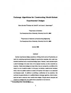
2.1 Coordinate systems We need several coordinate systems to locate the vehicle in space. Conversely to [114, p. 3] and [1], the inertial system x 0 , y0 , z 0 in Figure 2.1 is orientated in a way that the area spanned between x 0 and y0 is perpendicular to the vector of gravity (д). Through the large earth radius, the orientation of the inertial system changes only slightly during drive. Therefore, we can assume a quasi stationary inertial system. The road coordinate system is defined by x r , yr and z r . The inclination of the road surface with respect to д is expressed by road bank angle (ϕ r ) and the road angle (θ r ). A description of the rotational movement around z r is not essential and therefore omitted. Four wheels are rolling on the road surface. The wheel coordinate systems have their origin in the respective wheel center of gravity (CGW ), assuming ideal symmetric mass distribution for each wheel and wheel vertical axis (z W ) being normal to the road surface. Beside the three translational wheel degrees of freedom x W , yW and z W , we need the wheel camber angle (ϕ W ), wheel rotation angle (θ W ), and the wheel steer angle (δ W ). The body fixed vehicle coordinate system x V , yV and z V acts in the vehicle center of gravity (CGv ). The three angles are labeled with vehicle roll angle (ϕ V ), vehicle pitch angle (θ V ), and vehicle yaw angle (ψ V ). According to [1], CGv moves relative to the stationary system x 0 , y0 , z 0 with the vehicle velocity (v V ). Depending on the driving situation, we have to carry out certain coordinate transformations to obtain the vehicle velocity components in x V , yV and z V . In the easiest case of driving straight ahead without acceleration on a horizontal road surface we can adjust ϕ r = θ r = 0,
2 Vehicle force equilibrium zV δ W4 ϕV
ψV
z W4
xV
ϕ W4
CGv
x W4
CGW4
yV
ϕr z0
x0
xr
θV
yW4 y0
θr
yr road surface
θ W4
д
Figure 2.1: Vehicle with three translational (x V , yV , z V ) and three rotational degrees of freedom (ϕ V , θ V , ψ V ) which act in the body fixed vehicle center of gravity (CGv ). The directions x 0 , y0 of the inertial system create a surface which is perpendicular to д. The road coordinate system (x r , yr , z r ) is tilted with respect to this perpendicular surface around the angles ϕ r and θ r . The directions x W4 , yW4 and z W4 create one of four wheel coordinate systems which are numbered with index j W .
ϕ V = θ V = ψ V = 0 and therefore the vehicle velocity components become xÛV = v V and yÛV = 0.
2.2 Tire-road contact Friction ensures the force transmission between tire and road surface based on the relation F W = µ W FzW . The tire in Figure 2.2 is turned-in around δ W and moves with the velocity v W , whereby v W is twisted around the slip angle (α W ). This results in two force and velocity components F x W , FyW , xÛW , yÛW , respectively, with the relations vW =
8
q 2 + yÛ2 , xÛW W
2.3 Tire models FW =
q F x2W + Fy2W ,
FxW = µ xW FzW , Fy W = µ y W F z W , q µ W = µ x2 W + µy2 W . Note that the friction coefficients (µ x W , µyW ) depend on slip. Friction is partitioned in static friction (sticking) and kinetic friction (sliding). The deformation of the elastic tread blocks causes slip during sticking and a fraction of slip during sliding (assuming that the wheel still rotates). If static friction turns into kinetic friction, additional relative movements between the tread blocks and the road surface occur. Hence, kinetic friction causes higher slip than static friction. Following [114, p. 31] the lateral wheel slip (syW ) is defined as syW = tan α W =
v W sin α W yÛW = . v W cos α W xÛW
However, syW is only of minor importance in practice [114, p. 33]. Instead, α W is directly considered to determine the wheel lateral force. There are certain definitions for the longitudinal wheel slip (s x W ) . The piecewise defined relation (2.1) ensures that s x W remains within the interval of 0 ≤ s x W ≤ 1. ( θÛ r −xÛ W W W θÛWr W > xÛW propellingslip Û s x W = xÛ θ−WθrÛWr (2.1) W W W xÛW > θÛWr W brakeslip xÛW
θÛW is the wheel speed and r W the dynamic wheel radius. The definition for s x W by [122, p. 65] and [1] is given in (2.2). The longitudinal wheel slip becomes s x W = −1 while braking with locked tires and can increase to infinity while propelling sxW =
θÛWr W − xÛW . xÛW
(2.2)
In the following we use solely the slip definition of (2.2).
2.3 Tire models Tire models provide mathematical functions which describe the forces and torques in the tire road surface contact. Figure 2.3 shows typical character-
9
2 Vehicle force equilibrium
k xV δW
xW x˙W
αW
vW max(µ W )F zW
y˙W FyW yW
CGW
FW
FxW
Figure 2.2: Wheel longitudinal force (F x W ) and wheel lateral force (FyW ) in the tire road surface contact. Kamm’s circle (max(µ W )FzW ) saturates the wheel force (F W ). Accordingly, F W < max(µ W )FzW . Note that x V is parallel shifted from CGv into CGW .
1
� � F x W / max F x W
� � FyW / max FyW
1
0
0
−1
−1
a)
0 sxW
1
−1
−10
b)
0
10
α W in °
Figure 2.3: The wheel longitudinal force (F x W ) as function of longitudinal wheel slip (s x W ) and the wheel lateral force (FyW ) as function of slip angle (α W ) generated by the magic tire formula in (2.4).
10
2.4 Longitudinal vehicle forces istics for the functions F x W = f (s x W ) and FyW = f (α W ). Both curves can be approximated with a tangent around the zero point. This approach gives simple linear tire model FxW ≈ c xW sxW , Fy W ≈ c y W α W ,
(2.3a) (2.3b)
in which the two parameters c x W and cyW are the wheel longitudinal stiffness and wheel cornering stiffness, respectively. However model (2.3) is only valid in a narrow domain of definition around s x W ≈ 0 and α W ≈ 0. The curves of F x W and FyW show distinct inflexion points outside of the linear domain. Equation (2.4) shows a non-linear tire model which is known as magic tire formula [122, p. 165]. � � � B = X 3 sin X 2 arctan X 1A − X 4 (X 1A − arctan (X 1A)) (2.4) The measured output (B) can be F x W or FyW . Analogously, the measured input (A) is s x W or α W . The parameters (X 1 . . . X 4 ) are determined by experiments and specify the form of the function. Another often applied non-linear tire model was introduced by Burckhardt [26].
2.4 Longitudinal vehicle forces The following forces act in vehicle longitudinal axis (x V ) and apply in vehicle center of gravity or in the pressure point (PP). The pressure point is a point where all external aerodynamic forces can be combined in a single vector. 2.4.1 Climbing force Figure 2.4 shows a vehicle climbing a hill. The climbing force (F cl ) in (2.5), which acts in CGv , is determined by the vehicle mass (m V ), д and the gradient angle (θ ) [69, p. 155]. F cl = m Vд sin θ
(2.5)
While climbing a hill, the vehicle saves potential energy which is mainly transformed into kinetic energy (also partly transformed into electric and thermal energy) while driving downhill.
11
2 Vehicle force equilibrium xV xV
F cl
zV CGv
θ
θ mVд
m V д cos θ
Figure 2.4: Vehicle driving uphill. The forces that act in CGv are shown with magnification on the right.
2.4.2 Acceleration force Newton’s first law states that the translational acceleration of a mass causes a acceleration force (F ac ) which acts contrary to the direction of acceleration. F ac = m VvÛV
(2.6)
Commonly, (2.6) �comprises the reduced mass of rotational parts with F ac = 2 vÛ . However, the drive-train model model in Section 2.7 m V + I red (G)/r W V will consider the rotational parts. 2.4.3 Longitudinal aerodynamic resistance Figure 2.5 shows the longitudinal aerodynamic resistance (F x a ) which acts in the pressure point and originates through circulation and perfusion while driving straight ahead. In this case, v V = xÛV . The vehicle side slip angle (β V ) must be considered if the vehicle drives through corners. The dimensionless longitudinal drag coefficient (c x ) is determined with wind tunnel experiments which give the function c x over the air approach angle (ψ a ) (c x = f (ψ a )). Furthermore, the value on the ordinate c x (ψ a = 0) is often written as cw in literature. The longitudinal aerodynamic resistance becomes Fxa =
ρa AV (ψ a )v a2c x (ψ a ), 2
(2.7)
with the air density (ρ a ), vehicle cross-sectional area (AV ) and the air approach velocity (v a ) [69, p. 154]. The air density and the air approach velocity are affected by ambient conditions. If air is regarded as a dry ideal gas, the air density can be computed with the specific gas constant (R a ) R a = 287.058 J kg−1 K−1
12
2.4 Longitudinal vehicle forces Fya cx v V = x˙V
xV ψw
vw
PP
CGv
ψa va
Fxa cw
yV
ψa
Figure 2.5: Vektor superposition for the air approach velocity (v a ) for straight ahead driving [see 69, p. 153]. The common shape of the function c x = f (ψ a ) is shown on the right [see 69, p. 155]
by ρ a = pa /(R aTa ). The calculation of the exact air density is considerably more complex and exemplified in [127]. This calculation needs knowledge about the air pressure (pa ), air temperature (Ta ), molar masses of water, water vapor, a compression factor, and a molar gas constant. According to [69, p. 153], air approach velocity is given for straight driving in (2.8b) by summing up the vectors xÛV and wind velocity (v w ) and considering the wind angle (ψ w ). Note that even with solely side-wind (ψ w = 90°), the air approach velocity is larger than xÛV . � � cos(ψ w )v w − xÛV v®a = (2.8a) sin(ψ w )v w q 2 + 2xÛ v cos(ψ ) v a = xÛV 2 + v w (2.8b) V w w 2.4.4 Rolling resistance Haken [69, p. 150] explains that the rolling resistance (F Wr ) causes approximately 80 % of all resistances at the wheel while driving straight ahead on a dry and paved road. However, this reported fraction of F Wr depends strongly on air approach velocity. The analogous model of the wheel in Figure 2.6 exemplifies the origin of F Wr . The wheel vertical force (FzW ) causes the compression of the tire in the area of the road surface and an area of tread deflection is developed as a contact surface. Usually a parallel-connected spring damper model is used to describe the compressible characteristics of the air inside the tire and damping characteristics of the rubber [69, pp. 137–138]. During the deflection at the tire inlet, spring and damper act simultaneously. During the rebound at the
13
2 Vehicle force equilibrium zW θ ˙W
−F zW
xW
F Wr F Wr FzW eR
Figure 2.6: Tire analogous model [compare 155, p. 165].
tire outlet the spring force is reduced by the damper. Thereby the surface pressure at the tread is imbalanced. The resulting force FzW is shifted from z W about the distance e R to the front. A torque appears which counteracts to the rolling direction. The ratio of the two lever arms e R /r W is called coefficient of rolling resistance (f r ) which is required to compute the rolling resistance F Wr =
eR Fz = f r FzW . rW W
(2.9)
Note that (2.9) is a simplified equation to compute the rolling resistance because the rotational part of the wheel air resistance was assumed negligible. The coefficient of rolling resistance depends on the wheel vertical force, tire temperature, internal tire pressure, vehicle velocity, and the road surface [69, p. 139]. While driving on paved roads, the progressive influence of the velocity on f r is approximated in [114, p. 9] with f r (v V ) = f r 0 + f r 1v V + f r 4v V4 .
(2.10)
In the lower speed range v V 0 and accordingly, a resistance is introduced which is in principle comparable with the cornering resistance from Section 2.5.1. Mitschke and Wallentowitz [114, pp. 621–640] give a deeper introduction in vehicle sidewind dynamics.
2.6 Force equilibrium at wheel Let us balance all forces in circumferential direction at the wheel by the free body diagram of the wheel in Figure 2.8. The force equilibrium becomes F x V + F x W + F Wr = 0, TR − I WθÜW FxV = . rW
(2.16a) (2.16b)
The vehicle tractive force (F x V ) in (2.16b) includes the rim torque (TR ), the wheel rotation angle (θ W ), the wheel moment of inertia (I W ), and the dynamic wheel radius. The components of the rim torque will be explained in Section 2.7.
18
2.7 Drive-train
TB2 TE TG
TD
TB1
f (TG, θ˙G, G )
TR2
TG
θ˙ G
TR1
Figure 2.9: Drive-train of a two wheel drive vehicle with combustion engine and reardrive. The right side shows the qualitative shape of the loss-torque as function of torque and rotational speed for one gear of the manual gearbox.
We will use (2.16) to derive two vehicle tractive force models in Section 5.4.2 and Section 5.4.3. Moreover, Section 1.1 said that the prediction of the vehicle tractive force is the main objective of this work and (2.16b) gives the expression of the vehicle tractive force.
2.7 Drive-train The rim torque (TR ) is located at the internal section in Figure 2.8. Typically, it is expensive to measure TR directly. Accordingly, vehicle specific drivetrain models are used to determine TR out of the engine torque (TE ) [see 91, pp. 194–221]. A drive-train model describes the lossy torque transmission from the engine to the rim. Losses arise through friction within the drive-train. Often the friction losses of single components such as bearings, gearbox, or differential are described with characteristic maps which originate from experiments. The exact setup of the drive-train model depends heavily on the used components (electric motor, hybrid, conventional combustion engine, two wheel drive, four wheel drive, manual gearbox, automatic gearbox, . . . ). Therefore, it is impossible to find an uniform model structure for every thinkable drive-train and we will focus on one specific drive-train model. Figure 2.9 shows the drive-train of a two wheel drive vehicle with combustion engine and rear wheel drive. The engine torque is transformed in the gearbox and differential. We need to subtract the frictional losses which originate in this process at the gearbox output and differential output. While
19
2 Vehicle force equilibrium the clutch is engaged (θÛG ≈ θÛE ) the following relations give a drive-train model TG = TE ,
4 Õ
TD = TGi G (G) − f (TG , θÛG , G), θÛG θÛD = , i G (G) � TR, jW = TDi D − f (TD , θÛD ) − . . .
j W =1
· · · − I red (G)
4 Õ Ü + θ W2 Ü θ W1 − TB, jW , 2 j =1 W
I red =
4 Õ j W =1
I B, jW + i D2 I D + i D2 i G2 (G)(I G (G) + I C + I E ).
(2.17)
TG denotes the gearbox input torque, TD the differential input torque, TB denotes the braking torque, i G the gearbox ratio, G the gear, θÛG the derivative of the gear shaft rotation angle (gear shaft speed), θÛD the derivative of the differential shaft rotation angle (differential shaft speed), i D the differential ratio, I C the clutch moment of inertia and I E the engine moment of inertia. Here, it is assumed that all losses of auxiliary users (alternator, air conditioning compressor, . . . ) are already taken into account in TE . Moreover, (2.17) is shown in a short form (not all required rotational inertias are explicitely shown). The extended form of (2.17) considers all rotational inertias within the drive-train and it refers to θÛW . The wheel individual braking torque (TB, jW ) is given by TB, jW = pB, jW AB, jW r B, jW X B jW , [74, p. 171]. TB is dissipative in conventional vehicles with disc brakes but may be zero while non-braking, TB ≥ 0. X B includes the braking friction coefficient between the brake pads and the disk as well as the brake caliper efficiency. The braking friction coefficient is subject to strong variation, depending on disk temperature and preconditioning of the brake [157, p. 32]. This work assumes, that TR is available through a validated drive-train model for the used vehicle type. Thereby, all results can be transferred on similar vehicle types without further ado.
20
2.8 From equilibrium equations to models
2.8 From equilibrium equations to models Raising an equilibrium equation such as (2.16) is probably the standard method in engineering to deduce a model which approximates a mechanical system. A typical equilibrium is the force equilibrium j Õ
Fi = 0.
(2.18)
i=1
Now assume that we consider three forces in (2.18), hence j = 3 than (2.18) becomes F 1 + F 2 + F 3 = 0.
(2.19)
Let us suppose that F 3 is measurable. The vehicle tractive force from (2.16b) is for instance a measurable force if we use the drive-train model from Section 2.7. Let us further suppose that F 1 , F 2 are measurable up to unknown parameters X 1 , X 2 . Then we can rewrite (2.19) into A1,1X 1 + A1,2X 2 = B 1 , | {z } | {z } |{z} F1
F2
(2.20)
−F 3
where A are the measured inputs, X are parameters and B is the measured output. We can substitute for example the acceleration force of (2.6) for F 1 in (2.20) with A1,1 = vÛV and X 1 = m V and the longitudinal aerodynamic ρ resistance (2.7) for F 2 in (2.20), while A1,2 becomes v V2 and X 2 = 2a AVc x , assuming ψ a = 0. Equation (2.20) is linear in the parameters and because of that, (2.20) is a linear multi-input-single-output (MISO) model which comprises only two parameters. Hence, the model structure of (2.20) is rather simple. We are free to choose a more flexible model structure if we increase the number of considered forces in (2.18) (j > 3). Accordingly, we can create a set of candidate models from the force equilibrium (2.18) with different complexity. Commonly, X 1 and X 2 are only approximately known. Therefore, we try b1 and X b2 with an overdetermined system of equations and A1,1 , to estimate X A1,2 , and B 1 , turn from scalars into the matrix form At =1,1 At =2,1 .. . At =m,1
B t =1 At =1,2 � � B t =2 At =2,2 X 1 .. X ≈ .. . . . 2 B t =m At =m,2
(2.21)
21
2 Vehicle force equilibrium Now the rows of A and B contain measurements depending on the time (t). Note the ≈ symbol in (2.21). This symbol indicates that we expect some uncertainty in the measurement A or B or in both of them. If we assume uncertainty solely in B, (2.21) can be written as multi-input-single-output output-error model with matrix notation as b + ∆B, B = AX whereas ∆B is the output correction (see Section 3.5). If we assume uncertainty in A and B, the multi-input-single-output errors-in-variables model of Section 3.6 holds b + ∆B B = (A − ∆A)X and additionally considers the input correction (∆A). Each assumption of b. Moreover, we uncertainty requires an individual estimator to determine X can transfer (2.21) into a state-space output-error model bt = AX bt −1 + ∆X t X bt + ∆B t , B t = At X where the state matrix (A) considers knowledge about the temporal evolution of the parameters (see Section 3.7). No matter what kind of model we use (multi-input-single-output, statespace, output-error, errors-in-variables), we will treat each row in (2.21) as independent measurement. Hence, we will not consider a specific structure in A and B. However, most mechanical systems enforce a structure in A and B. Remember that we substituted the acceleration force for F 1 with A1,1 = vÛV and X 1 = m V . Hence, the measured vehicle acceleration (vÛV ) over time gives the column vector A:,1 . A plot of A:,1 would rather show a continuous function than a random signal, because the inertia of the vehicle causes that each row in A:,1 correlates with adjacent rows. Accordingly, it might be useful to expand (2.21) in a way that A and X become At =1,1 At =2,1 .. . At =m,1 22
At =1,2 At =2,2 .. . At =m,2
. . . . . . . . . . . .
X 1 B t =1 B t =2 X 2 ≈ .. . .. . . B t =m
(2.22)
2.8 From equilibrium equations to models The right block in the A-matrix of (2.22) could be filled with time-delayed measurements of some columns of A to consider the structure of A in the model. Moreover, we could fill this block with time-delayed measurements of B or ∆B to model the dynamics of unaccounted forces or to include a dynamical model of the output correction. Models which combine a deterministic part (left block in the A-matrix of (2.22)) and a part for the disturbance (right block in the A-matrix of (2.22)) are called auto regressive with eXogenous input (ARX). Isermann and Münchhof [86, p. 57] provide an overview for this model structure. In addition to this, [96] compares various ARX models for the errors-in-variables problem. Apparently, the number of parameters in (2.22) is larger than in (2.21). Hence, the identification as well as the prediction of ARX models becomes computational more expensive, which is the main reason why we will not continue to consider ARX models. On the other hand, this short introduction into ARX models might offer future research topics in vehicle parameter estimation. Summary: This chapter described major vehicle force components that are required to form a force equilibrium which is fundamental to deduce vehicle models. We will introduce various models and estimators in Chapter 3, where statistical assumptions and relations between different models are emphasized. Further, the introduction in vehicle dynamics within this chapter is useful to follow Chapter 4 (Survey of related research). In Chapter 5, we will use the force equilibrium of (2.16) and perform the same steps from (2.18) to (2.21) to deduce vehicle tractive force models.
23
.
3
Model s and estimators “Models [. . . ] are only approximations to unknown reality or truth; there are no true models that perfectly reflect full reality.” Burnham and Anderson [28, p. 264].
Outline: This chapter begins with an overview of various models and estimators. Than, we will introduce general concepts of model selection and model validation, followed by important methods with regard to regularization and robustness. Moreover, we will discuss linear gray-box models and their estimators in detail and emphasize transitions from one estimator into another. Besides, we will introduce novel recursive estimators which will generalize (include as special case) and improve common estimators. Several reproducible experiments with increasing complexity will indicate which estimator should be used for a specific problem. Afterwards, a novel estimator for a polynomial-function black-box model will provide an improved signal filter which will be used in Chapter 5 to smooth vehicle CAN signals. Finally, we will outline additional topics which might motivate further research. We will conclude this chapter with a guide for estimator selection. The deeper study of linear gray-box estimators within this chapter is required to evaluate related research in Chapter 4 and to interpret the results of the real world problem in Chapter 5.
3.1 Fundamentals Söderström and Stoica [168, p. 9] introduced the four concepts system, model structure, estimator and experimental condition which are useful to explain our degree of freedom with respect to system identification. The first concept system is the vehicle within this work. Usually, unmodified vehicles are desired. Hence, the system is given. In contrast, models are approximations of systems and we look often for models which describe the system response (output) for known input signals. Herein, we will focus on the vehicle longitudinal dynamics, precisely on models for the prediction of the vehicle tractive force. These models will be detailed in Section 5.4. Models can have different model structures, and some model structures have tunable parameters which can be adjusted through various estimators. An estimator is a mathematical procedure
3 Models and estimators to determine unknown model parameters from measurements. The weather belongs to the experimental condition, which is hard to control. Practically, it is impossible to conduct two test rides under the same weather condition. Hence, we should assume that the experimental condition is given. However, we are free to choose an appropriate model structure and estimator. Figure 3.1 gives an overview of various model structures and estimators. Starting from the root modeling, the three branches white-box, gray-box and black-box arise. We can differentiate these three categories by the amount of knowledge that each category requires to create models [86, p. 6]. First, white-box requires that everything about the system is known exactly to build a model. Therefore, we should be confident if we apply a whitebox model. Commonly, white-box models arise from differential equations. Differential equations are based on physical laws, such as energy conservation laws, conservation of mass (fluid mechanics), or force-torque equilibrium, as discussed in Section 2.8. A simple example is the description of motion of a spring mass damping system using a differential equation with the exactly known system-determining parameters mass, spring stiffness, and damping constant. Second, gray-box requires physical insight in the system but offers some degree of freedom in choosing the system-determining parameters. To be more specific, using a gray-box model means that we are uncertain in the parameters. Mostly, gray-box models ground on physical laws and thus, on differential equations. Although by nature usually non-linear, many technical systems can be adequately approximated by linear models. From here, we can choose between multi-input-single-output (MISO), random-walk (RW), and state-space (STSP). If the approximation by linear models is no longer valid, more challenging non-linear gray-box models are required with basically the same subcategories random-walk and state-space. Third, black-box means that we have no idea about the underlying physics of the system. Black-box models may be linear or non-linear and typical black-box models are impulse response (IR), polynomial-function (PF), neural networks (NN), and lookup tables. Lookup tables are often gained by measurements on test benches. The drive-train model of Section 2.7 for instance, is partly a black-box model with lookup tables for each gear. A lookup table is direct input-output mapping of data without the need to describe the data by mathematical equations. On the other hand, every time a lookup table is involved some kind of interpolation method is required for data which is not directly stored in the lookup table. The explanation up to here was about different model structures. If we
26
3.1 Fundamentals
EKF differential equations
UKF
white-box
non-linear
modeling
lookup table
PF, OE, L2
STSP
linear
BP EKF
SGF
RW MISO
NN, OE, L2 UKF
EIV Lρ
PKS LS
L2
OE, L2
Lρ
L2
KF SGIVMKF
Lρ
EIV
L2
OE OE
IVKF
EIV, L2
linear non-linear FIR
UKF
RW, OE, L2
gray-box
black-box
IR, OE, L2
EKF
STSP, OE, L2
RIVMKF IVMKF IVKF
Lρ
L2
RMKF
RRIVM
RIV RIVM
SGMKF
KF
MKF
TLS IV GTLS RRLM RGTLS RLM
WLS RLS
Figure 3.1: Model structures and estimators. shows explained methods, recursive algorithms and batch algorithms. L 2 depicts non-robust, L ρ robust estimators. The acronyms mean: backpropagation (BP), errors-in-variables (EIV), extended Kalman filter (EKF), finite impulse response (FIR), generalized total least squares (GTLS), impulse response (IR), instrumental variables (IV), IV Kalman filter (IVKF), IV M-Kalman filter (IVMKF), Kalman filter (KF), least squares (LS), multi-input-single-output (MISO), M-Kalman filter (MKF), neural networks (NN), output-error (OE), polynomial-function (PF), polynomial Kalman smoother (PKS), recursive GTLS (RGTLS), recursive IV (RIV), recursive IV M-estimator (RIVM), recursive M-estimator (RLM), recursive least squares (RLS), regularized M-Kalman filter (RMKF), recursive regularized IV M-estimator (RRIVM), regularized IV M-Kalman filter (RIVMKF), recursive regularized M-estimator (RRLM), random-walk (RW), Savitzky Golay filter (SGF), Stenlund-Gustafsson IV M-Kalman filter (SGIVMKF), Stenlund-Gustafsson M-Kalman filter (SGMKF), state-space (STSP), total least squares (TLS), unscented Kalman filter (UKF), weighted least squares (WLS).
27
3 Models and estimators measured inputs (A)
measured output (B)
system model
−
P
estimator
Figure 3.2: Block diagram of system, model (with a specific model structure), and estimator. Given the measurements, the estimator adjusts the model parameters, which is indicated by the dashed arrow. Disturbances are not shown [compare 45, pp. 3,8].
take a look further down of the gray-box or black-box branch in direction of the leaves, we discover that each model structure has various estimators. Herein, the estimator is nested under a model structure, considers statistical assumptions within a cost function, and provides an algorithm to estimate unknown parameters. Figure 3.2 visualizes the hierarchy of system, model with model structure, and estimator (batch or recursive algorithms) as general block diagram. Basically, the estimator adjusts parameters of a model with a given model structure. The estimator selects the model parameters in such a way, that the difference between measured output (B) of the system and the model output gives the smallest possible value of the cost function. Hence, estimation here means mathematical optimization. For instance, least squares (LS) is a batch estimator for the gray-box linear multi-input-single-output output-error model structure with L 2 cost function. Besides, there are recursive estimators which will be more important in the following for us. There is a distinct difference between white-box on the one hand, and graybox and black-box on the other. White-box models have not been adjusted by any kind of estimator, whereas gray-box and black-box models require estimators. As Figure 3.1 comprises such a great diversity of model structures and estimators, it makes sense to introduce at first some methods to examine the model quality, which allows us to compare different models.
3.2 Model selection and model validation Suppose we have a set of candidate models and want to compare these candidate models in terms of their model quality, then model selection gives the best
28
3.2 Model selection and model validation model inside the examined set of candidate models [100, p. 509]. However, the set of candidate models might not contain a useful model at all. Hence, we need model validation to test if this best model is good enough for the intended purpose, if it explains the measured output well, and if it is able to describe the hidden true system [100, p. 509]. Before we introduce numerous model structures and estimators we need to define a goal. Our aim is to find a good model. The dictum on Page 25 already answers the question if we can find a perfect model. On the first look, this dictum is discouraging. However, we know now that there is no optimal model and we can focus on finding a good model. So, what is good? Ljung [100, p. 492] as well as Söderström and Stoica [168, pp. 423, 438] defined two principles: flexibility and parsimony. Flexibility means “Is the model structure large enough to cover the [. . . ] system” [168, p. 423]? Parsimony means “Do not use extra parameters [. . . ] if they are not needed” [168, p. 438]. To sum up, a good model is flexible enough (gives small bias) and parsimonious (gives small variance). The bias-variance dilemma [73, p. 114] is a important concept in model selection. To explain the bias-variance dilemma, let us split a cost function (L) into a sum of bias and variance [100, p. 492] L = L bias + L variance .
(3.1)
One should choose the model inside the set of candidate models with the smallest L bias and L variance . However, in practice it turns out that small bias and small variance are hard to achieve simultaneously. Haykin [73, p. 114] explains the bias term as the inability of the model to describe the physics of the system. Generally speaking, more complex model structures cover the physics of the system better and reduce the bias. However, complex model structures comprise usually plenty parameters and introduce a lot of uncertainty for the estimator, because the information in the training data may be not sufficient to identify these plenty parameters accurately. Hence, model selection is always a trade-off between bias (or flexibility) and variance (parsimony). 3.2.1 Error-based performance indices We need measurable values (performance indices) to compare the model quality of different model structures and estimators. If the true parameters (X ) are known, we can compute the parameter error with the squared error vector
29
3 Models and estimators norm (SEVN)
2
bt
, SEVNt = X t − X 2
(3.2)
to observe which combination of model structure and estimator yields the b) [41, 53]. best estimated parameters (X Common choices to measure the model quality, in terms of the goodness b and measured output (B), are the mean of fit between estimated output (B) squared error (MSE), that gives an average over samples (m) in (3.3a) [100, p. 500], the normalized mean squared error (NMSE) in (3.3b) [100, p. 500] and the normalized root mean squared error (NRMSE) in (3.3c) [101, p. 8_15].
2 1
b
B − B 2 m
2
b
B − B 2 NMSE = 1 − kBk 22
b
B − B 2 NRMSE = 1 − kB − µ(B)k 2 MSE =
(3.3a) (3.3b) (3.3c)
The two latter ones vary from bad goodness of fit (−∞) to perfect goodness of fit (1) and measure how much of the measured output is explained by the model [100, p. 500]. 3.2.2 Candidate models How can we create a set of candidate models? First, we can define several candidate models from experience. Gray-box models require a certain knowledge of the underlying physics of the system. Hence, we can use this knowledge and setup some candidate models with increasing number of accounted forces for instance. In conclusion, the set of candidate gray-box models is commonly small and contains usually one useful model. However, we do not have much knowledge if we want to model a system with a black-box model. Hence, the second method is to create the set of candidate models rather randomly (trial and error). There are more sophisticated methods to estimate a useful model structure such as rank tests of covariance matrices and canonical correlation [100, pp. 495–498]. The rank test of covariance matrices relies purely on data and
30
3.2 Model selection and model validation yields parsimonious model structures without applying estimators. Canonical correlation is an iterative test if an additional parameter contributes to explain the measured output. Additionally, residual analysis is a method to test if the selected model structure is flexible enough. If the residual analysis shows high correlation between output correction and past measured inputs in (3.4a), the model could be improved by adding one or more past measured inputs. The correlation between output correction and past output correction in (3.4b) should be small. Otherwise the output correction depends on past data and the model structure needs improvement [100, pp. 511–514]. R ∆B,A;τ = R ∆B;τ =
m 1 Õ ∆B t At −τ m t =1
(3.4a)
m 1 Õ ∆B t ∆B t −τ m t =1
(3.4b)
3.2.3 Model selection with cross-validation Let us start with a thought experiment to highlight the superior characteristics of cross-validation in model selection. Suppose we have recorded noisy data from a system which we want to model. This data is the training data. Now we choose a suitable model structure and estimator. We identify a number of models with increasing model complexity (increasing number of parameters) from the training data and compute the goodness of fit for each model in terms of the MSE on the training data. It would turn out that the model with the highest model complexity (the most flexible model structure) yields the smallest MSE. As long as we increase the model complexity, the MSE will decrease further. Now we are in a trap which is known as overfit. The models start to explain the noise with increasing model complexity [100, p. 501]. We could even achieve perfect fit with a very complex model. Overfitting is very dangerous. So, let us study how cross-validation works to avoid overfitting. The simplest kind of cross-validation splits the recorded data into training data and validation data [100, p. 498]. Now we estimate the model parameters purely with the training data and compare the goodness of fit with the MSE for the validation data. Accordingly, we need to compute the estimated output for the validation data for each model and call this output the k step ahead prediction, where k is the number of prediction steps. As the validation data is
31
3 Models and estimators unseen for each model, the MSE on the validation data shows the prediction quality for each model. Hence, cross-validation delivers unbiased estimates of the cost function in (3.1) E(L) [100, p. 501]. Note that model selection with cross-validation is a pragmatic method. No assumptions about the system or statistics are required and models obtained from different estimators are comparable. Coss-validation has one drawback. The training data is smaller due to the split of the recorded data into training data and validation data. However, sometimes this drawback can be overcome by applying the estimator for a second time on all data (training data and validation data) with the previously selected model structure. 3.2.4 Model selection with information criteria Information criteria deliver the model quality without the need to portion the recorded data into training data and validation data. Hence, information criteria are the tools of choice if the recorded data from the system is expensive. However, information criteria rely on assumptions about statistics and vary with respect to the cost function of the estimator. Hence, it is not straight forward to compare different models which were gained by various estimators. While the derivation of the most common information criteria namely the Akaike’s information criterion (AIC) is given in [100, pp. 501–504], let us focus more on practical aspects in applying the AIC. AIC in (3.5a) provides a measurable value which accounts simultaneously for model quality and model complexity [27, p. 61]. The first term in (3.5a) measures model quality through the value of the cost function (L) and the second term the model complexity through the number of estimable parameters (o) which comprises the model parameters as well as parameters of the assumed statistical distribution. Note that AIC is given in (3.5a) without specific statistical assumptions. Equation (3.5b) gives AIC with the cost function for the least squares estimator [168, p. 442]. AIC = −2 log L + 2o ! m �2 1 Õ� bi AIC = m log Bi − B + 2o m i=1
(3.5a) (3.5b)
Generally, the smaller the AIC, the better the model. It is not the goal to find a model which memorizes the data, but to find a model that learns and captures the hidden information in the data [28, p. 275]. The pure AIC values are not directly applicable as they depend strong on the samples (m). According to
32
3.2 Model selection and model validation Table 3.1: Recommendation to evaluate the respectively model quality with ∆AICi [reproduced from 27, p. 70]. ∆AICi
support of model
0 to 2 4 to 7 >10
substancial considerably less essentially none
[27, p. 70], the AIC difference (∆AIC) is more meaningful to decide which model describes the hidden information superiorly. ∆AICi = AICi − min(AIC) The best model from the set of candidate models obtains a value of ∆AICi = 0. Table 3.1 gives recommendations how the respective ∆AICi are evaluated. Akaike’s information criterion can only compare the results of several models on the same record [27, p. 334]. Another often applied information criteria is the Bayesian information criterion (BIC) [27, p. 286] in (3.6a). The BIC gives the best model for prediction and grounds opposed to AIC on Bayesian theory. In (3.6b), BIC is given with the cost function for the least squares estimator. BIC = −2 log L + o log m ! m �2 1 Õ� b BIC = m log Bi − Bi + o log m m i=1
(3.6a) (3.6b)
The difference between AIC and BIC is explained in [27, pp. 293–301]. Basically, BIC compares the model quality purely with Bayesian theory and makes no assumptions about the true system whereas AIC tries to find the model which is close to the true system and makes assumptions about the system. The true model is not required in the set of models in the derivation of BIC [27, p. 295], whereas the derivation of AIC believes that a perfect model exists which is equal to the true system. Which information criteria is to be preferred depends strongly on the problem and there is no general rule if AIC or BIC is the better choice.
33
3 Models and estimators 3.2.5 Model validation Once we found the best model inside the set of candidate models via model selection, model validation provides confidence that this model works for the intended purpose. Remember, it might be that the set of candidate models does not include a useful model at all. Ljung [100, p. 509] highlights that the ultimate model validation is the successful application of the model. Basically, if the model works satisfactory all theoretic concerns about statistics, the model structure, and so forth are negligible. However, it is usually expensive and sometimes dangerous to validate a model directly at the intended application. Cross-validation from Section 3.2.3 is the superior method to validate a model [100, p. 510]. Accordingly, model selection with cross-validation yields the best and valid model from the set of candidate models in one step. Moreover, we established that gray-box models have parameters with physical meaning. Hence, if the parameter values, parameter variance, and the inputoutput sensitivity of the model confirms with prior knowledge of the system, convincing arguments are found that the model is reasonable [100, p. 509]. Before we begin to analyze the various model structures of Figure 3.1, we need to introduce two additional and important methods: regularization, and robustness.
3.3 Regularization Let us suppose we want to solve the overdetermined linear problem AX ≈ B
(3.7)
where A ∈ Rm×n is the measured input, X ∈ Rn×d are the unknown parameters and B ∈ Rm×d is the measured output. Problem (3.7) is an inverse problem. In practice, problem (3.7) is often ill-posed. Ill-posed means that the solution for X is sensitive to small variations in A and B [105], [160, p. 1]. Golub and Van Loan [63, pp. 80–81] explain that the measure of sensitivity can be evaluated by the condition number (c) of A. Let U SV = svd(A) be the singular value decomposition (svd(·)) of A, then the condition number becomes c = S 1,1 /S n,n , where S is the matrix of eigenvalues (S). The condition number is within range 1 ≤ c ≤ ∞ and the best possible condition number is one. If c � 1, problem (3.7) is ill-conditioned and the solution for X becomes unstable and may become meaningless [95, p. 1].
34
3.3 Regularization A problem is well-posed if Hadamard’s conditions Existence, Uniqueness and Continuity hold [73, p. 343]. Following the discussion of [73, p. 343], we can conclude that Hadamard’s conditions cannot be ensured if we apply recursive estimators. First, the existence criterion may be violated in that a distinct output may not exist for every input. Second, there may be not as much information in the training sample as we really need for a unique reconstruction of the input-output mapping [. . . ]. Third, the unavoidable presence of noise [. . . ] adds uncertainty to the reconstruction process [73, p. 343].
However, we will prefer recursive estimators instead of batch estimators, because batch estimators cause much computational burden. Practically speaking, problem (3.7) may become ill-conditioned or singular due to poor excitation of the measured inputs that is known as wind-up problem [68, 186]. One or more measured inputs show poor excitation if the persistent excitation condition ρ1I >
t +j Õ i=t
Ai>Ai > ρ 2 I
(ρ 1 , ρ 2 > 0) is not fulfilled [10, p. 136], [86, p. 250]. In short, poor excitation violates Hadamard’s existence criterion, because the input-output mapping contains only few information. Figure 3.3 provides an example where the true input (A) shows poor excitation between 50 s to 65 s. If A is noisy, the observations might contain pure noise and the solution for X becomes uncertain and unstable if exponential forgetting is applied, which is common in recursive estimators. Several approaches have been introduced to avoid wind-up [30, 50, 124, 145, 146, 171]. Regularization is a mathematical method mainly introduced through Tikhonov [173] to stabilize (smooth) the solution of ill-posed problems. The basic idea of Tikhonov regularization, which is also known as ridge regression, is to augment the cost function with a regularizer as shown in (3.8a). min L + κ kRX k 22
(3.8a)
min kB − AX k 22 + κ kRX k 22
(3.8b)
X X
Substituting L with the LS cost function in (3.8b) yields the basic regularized LS cost function with the regularization parameter (κ) and the regularization matrix (R) which is often set to the identity matrix (I ) [160, p. 7]. Other types
35
3 Models and estimators 1
A λ t −τ
0
−1
0
20
40
60
t in s
Figure 3.3: The true input A shows a mixture of rich excitation (10 s to 50 s) and poor excitation (50 s to 65 s). Exponential forgetting with the forgetting factor (λ) gives high weight to data where A shows poor excitation. Standard recursive estimators may suffer in this case under wind-up.
of R are extensively discussed in [95, pp. 12–21] and shortly introduced in [160, p. 7]. If κ = 0, (3.8b) turns into the basic LS cost function. The left hand side in (3.8a) can be replaced with other cost functions such as the total least squares (TLS) cost function as shown in [95, p. 1], [160, p. 45], [105], [182, pp. 57–66], and [103]. The larger κ, the smoother the solution for X becomes. However, a too large κ reduces the influence of L in (3.8a). Hence, the choice of κ is always a trade-off between a cost function and the regularizer (smoothness of X ). Often, we need to choose κ empirically. However, methods to adjust the optimal κ such as L-curve or cross-validation are explained in [160, pp. 11–13], [73, pp. 364–370], [34], [95, pp. 49–57], and [103]. Beside Tikhonov regularization other famous regularization methods are Levenberg-Marquardt regularization and Lasso, detailed in [186] and [172], respectively. Lasso favors sparse solutions through replacing the squared Euclidean norm by the 1-norm in the regularizer of (3.8b). Hence, Lasso with LS cost function becomes min kB − AX k 22 + κ kRX k 1 . X
3.4 Robust estimators Most estimators are based on statistical assumptions of distributions. LS is probably the most applied and studied estimator. Rousseeuw and Leroy [142, p. 2] explain the outstanding popularity of LS until nowadays with
36
3.4 Robust estimators two facts. First, LS has a closed-form solution which requires only simple matrix algebra. Second, LS yields the arithmetic mean of one dimensional data, which was around 1800 the most reliable location estimator. Notice that Gauss introduced the Gaussian distribution after defining the LS cost function so that LS is optimal for Gaussian distributed, zero mean output corrections [142, p. 2]. The LS cost function is min X
m Õ
(B i − Ai X )2
(3.9)
i=1
Í [82, p. 155]. Note that other references give (3.9) with 1/2(·), but this equation leads to the same solution. The references given by [142, p. 3] and [98] show, that many real world output corrections are non-Gaussian distributed. For instance, Clancey [38] examined around 250 distributions of chemical analysis and only 10 % to 15 % could be treated as Gaussian distributed. Zoubir et al. [200, p. 62] provide references where impulsive noise (Gaussian like distributions with heavier tails) was found in signal processing problems. But what happens if the output corrections are non-Gaussian? Many references show that LS fails to produce meaningful results if a single outlier is in the training data. Rousseeuw and Leroy [142, pp. 4,5] provide two examples of a straight line fit where a single outlier leads to corrupted parameters. A similar example is given by [200, p. 65]. Outliers can occur in the measured inputs (A) or in the measured outputs (B) [142, p. 5]. Applying the LS cost function, outliers in the measured inputs cause larger output corrections than outliers in the measured outputs. Outliers in the measured inputs are sometimes leverage points. In that case, they have a large influence on the LS solution. Rousseeuw and Leroy [142, p. 6] define a leverage point as a single point Ai , that lies far away from the majority of A. Hence, leverage points are not necessary outliers, but in any case they determine the LS solution strongly. Experiment 3.1
Call the function outliersLeveragePoints() with the string ’LS’ to compute the four LS straight line fits of Figure 3.4.
Figure 3.4 shows four straight line fits of seven data points with Gaussian e Each line fit is the result of LS estimation of the slope output noise (B). parameter, which has a true value of X = 3. Figure 3.4a does not contain outliers in the data. Hence, the LS solution in Figure 3.4a is precise and near
37
3 Models and estimators the true parameter. The accuracy of LS decreases significantly in Figure 3.4b with a single outlier in B 2 (the second entry of B). The original position of B 2 from Figure 3.4a is shown with an asterisk for convenience. The leverage point A4 (the fourth entry of A) in Figure 3.4c is an outlier and hence, the LS solution becomes meaningless. However, a good leverage point does not corrupt LS as shown in Figure 3.4d, where the seventh data point was moved far away from the other six data points. It was quite simple to find the leverage point in Figure 3.4c and Figure 3.4d. However, Rousseeuw and Leroy [142, p. 7] explain that it is impossible to uncover leverage points (and thus possible outliers) through simple visualization and inspection of the training data in higher dimensions. Outlier diagnostics provides data-based methods (no model is required) to uncover and remove outliers. Liang and Kvalheim [98] and Rousseeuw and Leroy [142, pp. 216–237] provide an overview of classic outlier diagnostics methods with a discussion of their common drawbacks (uncovered leverage points), whereas Knorr and Ng [93] and Rousseeuw and Leroy [142, pp. 237–245] introduce more recent and improved methods. The surveys [36] and [76] provide extensive introduction into outlier diagnostics. There is no general definition for outliers. Herein: Definition 3.1. An outlier is an observation that somehow deviates from the assumptions, mainly assumptions about the distribution. This definition matches well with the term robust. Huber and Ronchetti define robustness with: “robustness signifies insensitivity to small deviations from the assumptions” [82, p. 2]. Hence, robust estimators can deal with deviations from the assumptions or in other words can deal with a certain fraction of outliers. The breakdown point is a concept to measure robustness. Rousseeuw and Leroy [142, p. 10] explain the breakdown point as smallest fraction of outliers that cause the estimator to produce solutions that are arbitrarily far from the consistent solution. In accordance Huber and Ronchetti define the breakdown point as: The breakdown point is the smallest fraction of bad observations that may cause an estimator to take on arbitrarily large aberrant values [82, p. 8].
LS is non-robust and has a breakdown point of 0 %, whereas the highest possible breakdown point is 50 % [142, pp. 15, 126].
38
20
20
15
15
10
10
B
B
3.4 Robust estimators
5 0
5 0
10
0
20
A
0
10
20
A
a) no outliers
b) outlier in B 2
20
40
10
B
B
15 20
5 0
0
10
20
A
c) outlier and leverage point in A4
0
0
20
40
A
d) good leverage point
Figure 3.4: LS estimation ( ) of seven data points ( ) without outliers in Figure 3.4a, an outlier in the second entry of the measured output B 2 in Figure 3.4b, an outlier in the measured input A4 in Figure 3.4c which is also a leverage point and a good leverage point in Figure 3.4d. The asterisk ( ) shows the original data A4 , B 2 of Figure 3.4a. Similar figures can be found in [142, pp. 4–6] and [200, p. 65].
3.4.1 High breakdown point methods Huber and Ronchetti [82, p. 197] split robust estimators into robust methods and high breakdown point methods. High breakdown point methods seek to achieve the maximum breakdown point of 50 % but require often extensive computation or show a poor convergence. The convergence rate of LS is high 1 with m − 2 , if ∆B is Gaussian [82, p. 196]. Rousseeuw [139] introduced least median of squares (LMS) as high breakdown point estimator which can deal with outliers in the measured inputs and measured outputs. Therefore, LMS is robust in terms of bad leverage points (outliers in the measured inputs). The key idea in LMS is to replace the sum
39
3 Models and estimators in the LS cost function (3.9) with the highly robust median (med(·)). Hence, the LMS cost function becomes: min med(B i − Ai X )2 . X
i
(3.10)
The solution of (3.10) is expensive in matters of computation. Subsamples (tuples) of the training data are required as described in [142, pp. 197–204], where the LMS algorithm is shown. Furthermore, the convergence rate is 1 poor with m − 3 [82, p. 196]. Rousseeuw and Leroy [142, p. 15] introduced least trimmed squares (LTS) to overcome the problem with the poor convergence rate. LTS is as robust as LMS and has the same high convergence rate as LS. Rousseeuw and Leroy [142, p. 15] replaced the sum in the LS cost function with a trimmed sum: min X
j Õ
(∆B i )2 ,
(3.11)
i=1
b are the (first squared and than sorted) output corrections where ∆B i = B i −Ai X and j is the last considered sample from all m samples. Note that the LTS cost function (3.11) equals the LS cost function (3.9) if j = m. Hence, the largest output corrections are not considered in (3.11), which makes LTS robust but the additional sorting of the output corrections is even more pricy than the computation of the median in LMS. Rousseeuw and Leroy [142, pp. 206–208] outlined the root LTS algorithm with high computational complexity. However, the favorite properties of LTS, namely high convergence rate, a breakdown point of 50 % and robustness against outliers in measured inputs and measured outputs motivated numerous researchers to reduce the required computational burden [2, 14, 77, 144]. In spite of these enhancements, to best of my knowledge it has not been shown how to apply LMS or LTS as recursive estimator. There is one major reason why it is unlikely that LMS or LTS may be used recursively. LMS and LTS require to split the training data into tuples. On the contrary, recursive estimators must deal with an indefinite growth of measurements (m → ∞). How should we create all possible (or at least some) tuples if the training data is consistently growing? This is the reason why Figure 3.1 does not show LMS and LTS and why we focus on M-estimators from now on.
40
3.4 Robust estimators 3.4.2 M-estimators Huber [81] introduced M-estimators in 1964 with the idea to change the squares in the LS cost function with another function. Therefore, the M-estimator cost function looks similar like the LS cost function and becomes min X
m Õ
ρ(B i − Ai X ),
(3.12)
i=1
where ρ is a symmetric function preferably with a unique minimum at zero. LS is a special type of M-estimator. If ρ is set to ρ = (·)2 (or 1/2(·)2 , see the note on (3.9)), (3.12) turns into (3.9). Hence, the proper choice of the ρ-function determines the robustness of M-estimators. Taking the derivative of (3.12) with respect to X yields the set of equations � � m Õ B i − Ai X Ai, j = 0, j = 1, . . . , n, (3.13) ψ b σ (∆B) i=1 where ψ is the derivative of ρ with respect to ∆B (ψ = dρ/d∆B) and b σ is the inserted estimated scale that standardizes the output corrections [82, p. 161]. The estimated scale is needed because M-estimators are not scale-invariant. Accordingly, the estimated scale needs to be estimated simultaneously by a robust estimator and the common choice is the median absolute deviation (MAD) [141, 200] b σMAD (∆B) = 1.483 med |∆B − med ∆B|,
(3.14)
where the factor 1.483 was introduced to achieve a consistent estimator of the standard deviation for the Gaussian distribution. The cost function (3.13) requires iterative procedures because ρ and ψ are functions of the output corrections (∆B) and therefore of the desired parameters (X ). Iteratively weighted least squares (WLS) is the method of choice to solve (3.13) in practice, where the scaling matrix (W ) has to be computed at each iteration with W i,i =
ψi ∆B i /b σ (∆B)
until the estimated parameters remain sufficiently close together between the last and the current iteration. Algorithms of M-estimators, which are solved by iteratively WLS, are outlined in [82, p. 179], [98] and [21, p. 105].
41
3 Models and estimators We will use b σ as shorthand notation for b σ (∆B) in the following. Huber and Ronchetti [82, p. 174] suggest to use the following ρ-function and influence function (1 σ )2 σ | < δ, 2 (∆B/b � � for |∆B/b ρ(∆B/b σ) = (3.15a) δ δ |∆B/b σ| − 2 for |∆B/b σ | ≥ δ, ( ∆B/b σ for |∆B/b σ | < δ, ψ (∆B/b σ) = (3.15b) δ sgn(∆B/b σ ) for |∆B/b σ | ≥ δ, where ψ is saturated to δ if |∆B/b σ | ≥ δ . Contrary, ρ and ψ become for LS 1 σ )2 , ρ(∆B/b σ ) = (∆B/b 2 ψ (∆B/b σ ) = ∆B/b σ.
(3.16a) (3.16b)
We can see from (3.16b) that the influence function of LS is unbounded. Thus, LS is not robust if unusual large output corrections occur. Brabanter et al. [21, pp. 100–110] propose to use the highly robust Myriad function to deal with extreme outliers. However, the convergence rate is lower than for the Huber functions (3.15). Myriad was designed as maximum Likelihood scale estimator for the Cauchy distribution which is similar to the Gaussian distribution, but has heavy tails. Therefore, Myriad is a good choice in impulsive noise environments [see 64]. The Myriad ρ and ψ functions are � �� ln(10) 2 � � 2 β log β + (∆B/b σ )2 − log β 2 , 2 β 2 ∆B/b σ ψ (∆B/b σ) = . β 2 + (∆B/b σ )2 ρ(∆B/b σ) =
(3.17a) (3.17b)
Rather than [21, p. 105], I added in equation (3.17a) additional scaling terms to achieve a unique minimum at zero. Yet, these scaling terms are more of theoretical interest, because the derivative of (3.17a) leads to the same influence function (3.17b) as used in [21, p. 105]. Other ρ-functions are shown in [82, p. 99], [21, p. 105] and [158]. Figure 3.5 visualizes the properties of LS, Huber, and Myriad. First, the ρ-functions in Figure 3.5a show the transition from the LS cost function into the Huber cost function. If the output correction is larger than δ , the quadratic criterion turns into a linear, compare (3.16a) with (3.15a). Second, we can observe Huber’s intention directly in Figure 3.5b, where the influence functions
42
3.4 Robust estimators Myriad Influence function
Huber
ρ-function
LS
0 −δ
δ 0 −δ
δ
−δ
∆B/D σ
a)
b)
δ
∆B/D σ
weight (ψ /∆B)
1
0.5
0 −δ
c)
δ
∆B/D σ
Figure 3.5: Various ρ-functions in Figure 3.5a, influence functions in Figure 3.5b and the weight in Figure 3.5c.
are shown. LS has an unbounded influence function, whereas the Huber influence function is limited if the output correction is larger than δ . Myriad goes even further and gives gross output corrections decreasing influence. Third, Figure 3.5c gives the weight which is needed to fill the scaling matrix of iteratively WLS to solve (3.13). LS gives the same weight to all output corrections, Huber reduces the weight if |∆B| ≥ δ and Myriad shows a weight1 function which recalls the standard Cauchy distribution f (x; 0, 1) = π (1+x 2) . There is one drawback of M-estimators compared with the LMS and LTS high breakdown point estimators. M-estimators are not robust in terms of bad leverage points. Actually, this fact motivated Rousseeuw to develop LMS and LTS although generalized M-estimators were introduced to improve the robustness of M-estimators [for further detail consult 139, pp. 12–14]. Cases
43
3 Models and estimators where M-estimators fail because of one or more bad leverage points are shown in [139, 200]. Accordingly, the breakdown point of M-estimators is 0 %. Figure 3.6 is the robust counterpart of Figure 3.4. The same data was used. The Huber tuning constant was δ = 1.345 and the Myriad tuning constant β = 1. All robust estimators produce close results in Figure 3.6a and in Figure 3.6b, where LS showed a corrupted result (Figure 3.4b). Figure 3.6c shows the difference between a high breakdown point estimator (LMS) and a robust estimator (M-estimator). Both M-estimators perform not better than LS in Figure 3.4c. Yet, the Myriad M-estimator is slightly better than the Huber M-estimator. However, if the leverage point moves slightly more to the right, Myriad and Huber give close unsatisfactory results, whereas the performance of LMS remains superior. Experiment 3.2
Call the function outliersLeveragePoints() with the string ’robust’ to compute the four robust straight line fits of Figure 3.6. Modify the position of the bad leverage point in line 20 of outliersLeveragePoints() to bring the Myriad M-estimator to its breakdown.
On the other hand, we have seen in Figure 3.6b that M-estimators are highly robust against outliers in the measured output. Furthermore, Huber and Ronchetti remark: It appears that M-estimates offer enough flexibility and are by far the easiest to cope with, simultaneously, with regard to computation, asymptotic theory, and intuitive interpretation; moreover, the step from [. . . ] [(3.9) to (3.12)] is easily explainable to nonstatisticians also [82, p. 164].
RRLM
Lρ
RLM
Let us add to this convincing comments the feature that M-estimators are an ideal source to develop recursive estimators. That is due to the relation between (iteratively) WLS and recursive least squares (RLS), where the latter will be the first presented recursive estimator in Section 3.5.3. Moreover, Mestimators are a vital part of other popular high breakdown point methods such as the MM-estimator [195] which performs superior in some signal processing applications as discussed in [200].
MISO OE L2
RLS WLS
LS
3.5 Linear multi-input-single-output output-error model The first presented gray-box model is the linear multi-input-single-output output-error model. The respective branch from Figure 3.1 is shown in the margin for convenience. The model structure was already introduced in (3.7) and is detailed here with output corrections AX ≈ B,
44
e B = B + B,
(3.18a)
3.5 Linear multi-input-single-output output-error model 20
20 15 LMS M-Huber M-Myriad
10 5 0
0
10
B
B
15
10 5 0
20
A
0
10
20
A
a) no outliers
b) outlier in B 2
20
40
10
B
B
15 20
5 0
0
10 A
20
c) outlier and leverage point in A4
0
0
20
40
A
d) good leverage point
Figure 3.6: Robust estimation of the same data as in Figure 3.4. All estimators are close in Figure 3.6a and Figure 3.6d. Figure 3.6b shows the benefit of robust estimators compared with Figure 3.4b where LS failed. The outlier and leverage point in Figure 3.6c leads to a breakdown of the M-estimators. LMS is superior.
b + ∆B, B = AX
(3.18b)
b with ∆B ∈ Rm×d . The number where the output correction is ∆B = B − B of outputs (d) is one, because we consider the single-output case (d = 1). Model structure (3.18) considers perturbation only in B (output-error). Hence, (3.18) is a constrained perturbation problem. No corrections are applied in A. e is assumed with Therefore, the noise covariance matrix (P) �� �� �� � � e B e = σ 2 diag 0 0 . . . 1 > , Pe = cov A (3.19) where cov(·) is the covariance operator and diag(·) extracts diagonal elements of a matrix or converts a vector into a diagonal matrix.
45
3 Models and estimators 3.5.1 Least squares The well known LS closed-form solution for problem (3.18) becomes � b = A>A −1A> B X (3.20) � � b)(X − X b)> [37, p. 4]. The covariance of parameter estimation error E (X − X (denoted as covariance matrix (P) in the sequel) is commonly computed with > ∆B P =b σ 2 (A>A)−1 and b σ 2 ≈ ∆B m−n [168, pp. 65–66]. Proof. We can rewrite the LS cost function (3.9) in matrix notation min kB − AX k 22 X
(3.21)
and follow Söderström and Stoica [168, pp. 62–63] to present (3.21) in the equivalent form L = (B − AX )> (B − AX ), � = B > − X >A> (B − AX ), = B > B − B >AX − X >A> B + X >A>AX . The following intermediate step explains how to compute the derivative for the rightmost term of the cost function. d > > d ∗> ∗> 0 0 d ∗> ∗> 0 0 X A AX = X A AX + X A AX , dX dX ∗ dX 0 � > = A∗>A0X 0 + X ∗>A∗>A0 , = A∗>A0X 0 + A0>A∗X ∗ , = 2A>AX . Accordingly, the complete derivative of the cost function becomes �> dL = 0 − B >A − A> B + 2A>AX , dX = −2A> B + 2A>AX . Setting this derivative to zero, the solution for X becomes (3.20).
�
LS is the maximum-likelihood estimator for (3.21) if the conditions which were discussed in Section 3.4 and [86, p. 254], hold. Mainly, the output corrections may not be correlated and have E(∆B) = 0.
46
3.5 Linear multi-input-single-output output-error model 3.5.2 Weighted least squares We have already discussed WLS in Section 3.4.2, where iteratively WLS was used within M-estimators. The cost function of WLS offers more flexibility than LS due to the introduced scaling matrix and becomes
2
√
(3.22) min W (B − AX ) , 2
X
where W is a positive diagonal matrix of dimension W ∈ Rm×m . The WLS closed-form solution becomes b = (A>W A)−1A>W B X
(3.23)
[86, p. 279] and we can see that LS is a special case of WLS when the scaling matrix is equal to the identity matrix (W = I ). 3.5.3 Recursive least squares The RLS algorithm in Algorithm 3.1 is the recursive version of WLS with a special form of scaling matrix. The diagonal elements of the scaling matrix decrease exponentionally over time, which is also known as exponentionally forgetting. Hence, the scaling matrix has the form � �> diag(W ) = λt −1 . . . λ2 λ1 λ0 and the RLS cost function becomes min X
m Õ
λm−i (B i − Ai X )2
(3.24)
i=1
[100, pp. 363, 364]. The forgetting factor (λ) (0 � λ ≤ 1) controls how much weight is given to old data. If we adjust λ = 1, RLS solves the LS cost function (3.9), where all data is considered with equal weight. Figure 3.3 showed already how λ evolves over time if λ < 1. Ljung [100, pp. 363–365] gives the transition from (3.22) into Algorithm 3.1 by using the matrix inversion lemma, whereas Isermann and Münchhof [86, pp. 281–283] derive Algorithm 3.1 by iterative inserting new data and updating the WLS solution in (3.23). If RLS is just another algorithm which does the same as LS or WLS with a special design of W , why do we discuss RLS and various more recursive estimators in the following? The reasons why we should favor recursive estimators are:
47
3 Models and estimators Algorithm 3.1: Recursive least squares (RLS) for t ← 1 to m do bt −1 , P t −1 , At , B t , λ input: X � � −1 2 Lt = P t −1At> λ + At P t −1At> � � bt = X bt −1 + Lt B t − At X bt −1 3 X 1
P t = (I − Lt At )P t −1 λ1 bt , P t output: X
4
1. the number of mathematical operations does not depend on m, hence we can process infinite large data sets; 2. the required storage is fixed and known from t = 0 s onwards; b for each time-step t; 3. we get a solution X 4. recursive algorithms can follow and track time-varying systems; 5. and because of that, recursive algorithms are ideal for real-time applications, such as vehicle control. Recursive estimators can be shown as individual equations or as algorithms. Rather than individual equations, I favor to present recursive estimators as algorithms because recursive methods require initialization of some values and constants, a certain sequence of computations, and deliver results at each time-step. For instance, we can see in Algorithm 3.1 that RLS requires the initial values bt −1 , P t −1 (both appear at the input line); a constant λ (no index t) and provides X bt , P t as result for each time-step. X 3.5.4 Recursive M-estimator The end of Section 3.4.2 indicated already that M-estimators, WLS, and RLS are connected and we have seen the need for robust estimators in Section 3.4. The recursive M-estimator (RLM) was discovered more than once. Dai and Sinha [40] is, to the best of my knowledge, the first reference that gives an RLM algorithm without forgetting factor. They were followed by Zou, Chan, and Ng [199], who proposed the same core algorithm but included a forgetting factor in the RLM cost function min X
48
m Õ i=1
λm−i ρ(B i − Ai X ).
(3.25)
3.5 Linear multi-input-single-output output-error model Algorithm 3.2: Recursive M-estimator (RLM) for t ← 1 to m do bt −1 , P t −1 , At , B t ,W t,t , λ input: X � � −1 2 Lt = W t,t P t −1At> λ + W t,t At P t −1At> � � bt = X bt −1 + Lt B t − At X bt −1 3 X
1
4
P t = (I − Lt At )P t −1 λ1 bt , P t output: X
The derivation from (3.25) into Algorithm 3.2 was done by [199] through the matrix inversion lemma. Algorithm 3.2 differs from Algorithm 3.1 in the introduced time-dependent weight W t,t , that is a scalar, denoted by the double indexing. As discussed in Section 3.4.2, RLM covers RLS as special case if the weight is adjusted to W t,t = 1, ∀t. It is straight forward to apply (3.15b), (3.17b) or other influence functions to compute the weight with W t,t = ψ t /∆B t . However, we know from (3.13), that we need a simultaneous robust method for the estimated scale. Zou, Chan, and Ng [199] suggested � b σt2 = λb σt2−1 + (1 − λ)1.483 1 +
� j 5 med ∆B t2−i , j − n i=0
(3.26)
which is a sliding-window version of the first equation in [142, p. 44]. However, (3.26) requires to store j squared output corrections in a memory and to compute the median of them. This procedure is not computational efficient because of the memory size j which is needed to compute the estimated scale. Moreover, the median requires to sort all j entries. Consequently, one would always have to balance between large-j, which is good for statistics and smallj, which is computational cheaper. Hence, (3.26) leads into a dilemma. The same problem arises if we would use the robust MAD from (3.14) to compute the estimated scale. Rousseeuw and Bassett [140] suggested to replace the median with the repeated median for large data sets. The repeated median performs nested median operations with hierarchical ordered small buffers and is computational more efficient than the conventional median. Although the repeated median is an improvement over the conventional median, we should seek for a robust scale estimator which has comparable computational load as the non-robust standard deviation (3.27a) and its
49
A
3 Models and estimators recursive version (shown as variance in (3.27b)) v t b σ=
m 1 Õ 2 ∆B i , m − n i=1
b σt2 = λb σt2−1 + (1 − λ)∆B t2 ,
(3.27a) (3.27b)
[140, p. 40] and [199], respectively. More explanation for the recursive standard deviation can be found in [35, 191]. Bylander and Rosen [29] presented an recursive median algorithm which grounds on perceptron learning-algorithm [138]. The idea is to use some estimated median from the previous time-step, compare it with incoming data, and correct the estimate in direction of steepest descent with the learn rate (η). Further, Bylander and Rosen [29] explain a slight modification which b for any desired probability (p) (the median is delivers estimated quantiles (Q) the quantile on 0.5 probability) and this modification makes their algorithm general. The estimated quantile of the squared output correction is gained by b + 2ηp bt −1 , Q if ∆B t2 > Q t −1 bt = Q bt −1 bt −1 , Q if ∆B t2 = Q 2 b b Q t −1 − 2η(1 − p) if ∆B t < Qt −1 ,
(3.28)
and delivers the recursive median, if we adjust the probability to p = 0.5. The learn rate (η) ranges typically between 0.001 to 0.01 and determines the convergence rate of the estimator. An equivalent formulation without piece-wise definition is bt = Q bt −1 + η|sgn(∆B 2 − Q bt −1 )|(sgn(∆B 2 − Q bt −1 ) + 2p − 1). Q t t
(3.29)
bt of Replacing everything right of the scaling factor 1.483 in (3.26) with Q (3.29) yields the desired robust estimated scale which is required to run RLM as shown in Algorithm 3.3. First, the normalized a priori output correction (∆B t ) is computed with b from the previous time-step in Line 2. Second, Line 3 and Line 4 estimates of X yield the weight based on the a priori output correction and the estimated b and P for the current scale from the previous time step. Third, RLM gives X time-step. Fourth, the a posteriori output correction in Line 7 is used to update the robust estimated scale in Line 8–Line 9.
50
3.5 Linear multi-input-single-output output-error model Algorithm 3.3: RLM with robust estimated scale for t ← 1 to m do bt −1 , At , B t , λ, η, p = 0.5 bt −1 , P t −1 , b input: X σt2−1 , Q bt −1 ) 2 ∆B t = (B t − At X ( (3.15b), or 3 ψ t (∆B t /b σt −1 ) = (3.17b) ψt 4 W t,t = ∆B t /b σt −1 5 function call bt −1 , P t −1 , At , B t ,W t,t , λ input: X 6 RLM (Algorithm 3.2) bt , P t output: X bt 7 ∆B t = B t − At X b b bt −1 )|(sgn(∆B 2 − Q bt −1 ) + 2p − 1) 8 Qt = Qt −1 + η|sgn(∆B 2 − Q 1
t
bt b σt2 = λb σt2−1 + (1 − λ)1.483Q bt bt , P t , b output: X σ 2, Q
9
t
t
Algorithm 3.3 gives the same result as RLS if we use the influence function of LS (3.16b) in Line 3. Further, we can simplify Algorithm 3.3 if a user-defined fixed estimated scale is given. Then, Line 7–Line 9 can be omitted. Note that Algorithm 3.3 grounds on the implicit assumption that one iteration per time-step is sufficient. In other words, Algorithm 3.3 is a suboptimal estimator for (3.25). However, Algorithm 3.3 can be modified into an optimal bt conestimator through multiple iterations of Line 2–Line 9 for each t until X verges. Remember that the cost function in (3.13) requires iterative procedures (iteratively WLS), as discussed in Section 3.4.2. 3.5.5 Recursive regularized M-estimator Remember the reasons for applying regularization which were discussed in Section 3.3 and let us write once again the cost function (3.8b) for LS with Tikhonov regularization as sum with exponential forgetting min X
m � Õ
� λm−i (B i − Ai X )2 + κ kRX k 22 ,
(3.30)
i=1
51
3 Models and estimators where R = I . Now let us replace the squares in (3.30) with the ρ-function to derive the recursive regularized M-estimator cost function min X
m Õ
� λm−i ρ(B i − Ai X ) + κ kRX k 22 .
(3.31)
i=1
The regularizer (right hand side in (3.31)) adds a bias towards zero and prevents b becoming suspicious large. Hence, the estimation variance (or uncertainty) X is reduced during poor excitation [186]. Van Waterschoot, Rombouts, and Moonen [186] give the batch solution for Tikhonov regularized LS (3.8b) b = (A>A + κI )−1A> B, X
(3.32)
where, compared with the LS solution (3.20), a scaled identity matrix is added to the input covariance matrix (R) (R = A>A). Further, the recursions for the input covariance matrix and estimated parameters become R t = λR t −1 + A>t At + (1 − λ)κI , � � bt = X bt −1 + R t−1 A>t (B t − At X bt −1 ) − (1 − λ)κ X bt −1 X
(3.33a) (3.33b)
[186]. However, the inversion of R in (3.33b) should be avoided by the matrix inversion lemma similar to RLS and RLM in Algorithm 3.1 and Algorithm 3.2 respectively. Additionally, let us condense the term (1 − λ)κ into a scaled κ. Gunnarsson [68] showed that the inversion of the input covariance matrix P = R −1 of (3.33a) leads to a normalization of the covariance matrix P after the P-update P t0 = P t (I + κP t )−1 , A
(3.34)
where P t0 is the regularized covariance matrix. The combination of (3.33), (3.34), and Algorithm 3.2 leads to the recursive regularized M-estimator (RRLM) with the two regularization methods Levenberg-Marquardt regularization and Tikhonov regularization in Algorithm 3.4. The Levenberg-Marquardt regularization (also shown in [186]) differs from Tikhonov regularization in the computation of the parameter update. Levenberg-Marquardt regularization causes that the parameters remain at their values during poor excitation, whereas Tikhonov regularization causes that
52
3.5 Linear multi-input-single-output output-error model Algorithm 3.4: Recursive regularized M-estimator (RRLM) for t ← 1 to m do bt −1 , P t −1 , At , B t ,W t,t , λ, κ input: X � � −1 2 Lt = W t,t P t −1At> λ + W t,t At P t −1At> 1 3 P t = (I − Lt At )P t −1 λ 4 P t = P t (I + κP t )−1 5 switch type do 6 case Levenberg-Marquardt regularization do � � bt = X bt −1 + Lt B t − At X bt −1 7 X 1
case Tikhonov regularization do � � bt = X bt −1 + Lt B t − At X bt −1 − P t κ X bt −1 X
8 9
bt , P t output: X
the parameters tend towards zero during poor excitation. RRLM turns into RLM if κ = 0. Hence, RLM and RLS are included as special cases in RRLM and we can substitute RLM (Algorithm 3.2) in Line 6 of Algorithm 3.3 with RRLM to create a flexible recursive regularized robust estimator for the linear multi-input-single-output output-error model. 3.5.6 Experiments Let us conduct a sophisticated experiment to study the properties of RRLM in conjunction with the robust estimated scale with different settings of Algorithm 3.4 inside Algorithm 3.3. Figure 3.7 shows the measured inputs and measured output which were generated with � t= 1
2
3
... m
�>
, m = 10 000 s,
A:,1 = sin(2π t 0.006) sin(2π t 0.006/3.3),
A:,2
sin(2π t 0.012) sin(2π t 0.012/3.3) 1 s ≤ t < 1000 s 0 1000 s ≤ t < 6000 s = , sin(2π (t − 5000)0.012) sin(2π (t − 5000)0.012/3.3) 6000 s ≤ t ≤ 10 000 s
A:,3 = sin(2π t 0.014) sin(2π t 0.014/3.3),
53
3 Models and estimators A1
2
A2
A3
B 5 B
A
0 −2
0 −5
600
800
1,000
1,200
600
800
1,000
1,200
t in s
t in s
b)
a)
Figure 3.7: Measured inputs (A) and measured output (B) modeled as sine waves [altered from 133]. A1 , A2 , and A3 are noise free, whereas B has additive white Gaussian noise. A2 shows no excitation between 1000 s to 6000 s. All signals contain outliers.
X 1:3,:
h i> 1 2 3 i> = h 1.5 2 3
1 s ≤ t < 5000 s 5000 s < t ≤ 10 000 s
,
B = A�X
[altered from 133]. All measured inputs are noise free (A = A), whereas B contains additive white Gaussian noise with zero mean and 0.1 variance. Further, A and B contain 5 % outliers, that were built from uniform random numbers ranging from −4 to 4. A2 shows no excitation (remains constant) between 1000 s to 6000 s and � is the element-wise product which is also known as Hadamard product. The step change in X 1 at t = 5000 s creates a time-varying system. Experiment 3.3
Call the function linearMISOoe() four times with the strings ’RLS’, ’RLM’, ’LevenbergMarquardt-RRLM’ and ’Tikhonov-RRLM’ to compute the four parameter estimates in Figure 3.8. Algorithm 3.3 with Algorithm 3.4 in Line 6 (RRLM with robust estimated scale) will be executed with λ = 0.995 for all cases. The regularization parameter is adjusted to κ = 0 for ’RLS’ and ’RLM’, κ = 0.1 for ’Levenberg-Marquardt-RRLM’ and κ = 0.001 for ’Tikhonov-RRLM’. The influence function is (3.16b) for ’RLS’ and (3.15b) for all other cases.
Figure 3.8a shows RRLM in a setting that is identical to basic RLS. The solution is heavily distorted through outliers in A and B. Hence, RLS is not able to produce meaningful results for Experiment 3.3.
54
3.5 Linear multi-input-single-output output-error model D1 X
4
D2 X
D3 X
D X
2
0
a) ’RLS’
b) ’RLM’
4
D X
2
0 0
0.5 t in s
1 ·104
c) ’Levenberg-Marquardt-RRLM’
0
0.5 t in s
d) ’Tikhonov-RRLM’
1 ·104
Figure 3.8: Estimated parameters for four different settings of RRLM. Nominal values are shown with lines.
The result of the robust RLM estimator with Huber’s cost function is shown in Figure 3.8b. The estimates are more stable than in Figure 3.8a. However, b2 becomes uncertain for t = 5000 s to 6000 s. This uncertainty is known as X wind-up problem. A2 was set to zero for t = 1000 s to 6000 s, which leads to an ill-posed problem. However, the estimator keeps an exponentially decreasing amount of old information until t ≈ 5000 s, which explains the delay between b2 at the beginning of zero excitation of A2 at t = 1000 s and the wind-up of X t ≥ 5000 s. Compare also with Figure 3.3. Figure 3.8c and Figure 3.8d show the result of RRLM with two different regularizations. The difference between Levenberg-Marquardt regularization in Figure 3.8c and Tikhonov regularization in Figure 3.8d is that Tikhonov b2 towards zero when A2 ≈ 0 between 1000 s to 6000 s, regularization forces X b2 in this period constant. whereas Levenberg-Marquardt regularization keeps X Tikhonov regularization is in this case a kind of feature selection, because any
55
3 Models and estimators ’RLS’ ’RLM’
’Levenberg-Marquardt-RRLM’ ’Tikhonov-RRLM’
SEVN
102
10−1
10−4
0
0.5
a)
t in s
1 ·104
0
0.5 t in s
b)
1 ·104
Figure 3.9: Squared error vector norm for four different settings of RRLM.
b2 would lead to A2X b2 ≈ 0 if A2 ≈ 0. Hence, we could discard A2 and X b2 for X t = 1000 s to 6000 s without loosing accuracy of the model. The same conclusions can be derived from Figure 3.9 where the SEVN is shown for all four settings of Experiment 3.3. However, the SEVN (3.2) allows to compare various estimators without the need to show all parameters explicitly. Hence, SEVN will be used as performance index for the parameter error from this point onwards. Figure 3.9a shows that the squared error vector norm of RLM is significantly lower than RLS. Furthermore, the wind-up around t = 5000 s is well visible. The two different regularization methods of RRLM in Figure 3.9b lead to a more stable solution when A2 has no excitation. However, in terms of SEVN, the Levenberg-Marquardt regularization is the far better choice in comparison to Tikhonov regularization. Finally, Figure 3.10 gives the estimated scale in Figure 3.10a as well as the weight in Figure 3.10b for the RRLM estimator with Levenberg-Marquardt regularization. The robust estimated scale of Line 8–Line 9 in Algorithm 3.3 yields sufficient accurate scale estimates with fast convergence, see Figure 3.10a. To sum up, we can conclude that M-estimators in conjunction with an appropriate regularization method lead to superior accurate parameter estimates, although M-estimators are not robust against bad leverage points as discussed at the end of Section 3.4.2. The results of Experiment 3.3 indicate that M-estimators are sufficient robust for practical needs.
56
3.6 Linear multi-input-single-output errors-in-variables model 0.6 weight (ψ /∆B)
1
σ D
0.4 0.2 0
0.5
a)
t in s
1 ·104
0.5
0
600
800
b)
1,000
1,200
t in s
Figure 3.10: Estimated scale in Figure 3.10a and weight in Figure 3.10b of the RRLM estimator with the setting ’Levenberg-Marquardt-RRLM’.
3.6 Linear multi-input-single-output errors-in-variables model Let us switch now to the next branch of Figure 3.1, as denoted by the figure on the margin. The linear multi-input-single-output errors-in-variables (EIV) model AX ≈ B,
e A = A + A,
b + ∆B, B = (A − ∆A)X
e B = B + B,
(3.35a) (3.35b)
e and output noise (B). e In other considers in contrast to (3.18) input noise (A) words, it is assumed that all signals have some uncertainty. Therefore, problem (3.35) is an unconstrained perturbation problem, more general than (3.18), and comprises the latter one as special case. Generally speaking, errors-invariables estimators are more complex than output-error estimators. This drawback is compensated by the reduced parameter bias of errors-in-variables estimators that has been observed in numerous studies if the constrained perturbation assumption of (3.18) does not hold [37, 41, 49, 53, 94, 106, 116, 133, 134, 164, 166], [73, p. 116], [86, pp. 302–304], and [185, p. 5]. Reused material: Errors-in-variables estimators can be divided into two classes. The first class requires knowledge of the noise covariance matrix. The bias-compensating RLS algorithm by [44] adds a correction term which is built from the noise variance and a correlation matrix and adjusts the estimates. Furthermore, numerous recursive TLS (RTLS) algorithms based on the minimization of the Rayleigh quotient were proposed by [7, 41, 54, 55, 99]. All of these methods try to solve the errors-in-variables problem [(3.35)]
57
RIVM RRIVM Lρ MISO EIV
RIV L2
TLS
IV
RGTLS
GTLS
3 Models and estimators with a cost function that considers data corrections in all elements of the augmented data (Z ). In the second class, the bias in the estimated parameters is reduced by properly chosen instruments (A). A recursive total instrumental variables (RTIV) estimator was introduced by [54]. The main advantage of instrumental variables (IV) methods is that no knowledge of the noise covariance matrix is required [This reused material has been reformatted for uniformity. ©2014 IFAC. 133]. However, IV methods impose other assumptions. Essentially, the instruments should be chosen in a way that they are uncorrelated with input noise and output noise, but maximally correlated with the measured inputs. The simplest way to yield proper instruments is to use time-delayed measured inputs. Anyhow, we will discuss IV methods in detail in Section 3.6.4. 3.6.1 Total least squares (TLS)* Reused material: Markovsky and Van � Huffel� [106] � pointed � out � that� b B b TLS searches for optimal data corrections ∆A ∆B := A B − A (3.36), where k·kF denotes the Frobenius norm. � �
� � � � � �
A B − A b B b s.t. A b B b X = 0 (3.36) min F −I m×q b B]∈R b X ∈Rq×d ,[A bX b= The approximate solution of the overdetermined system of equations is A b If the noise is independently identically distributed with zero mean and a B. covariance matrix �� �� e B e = σ 2I , Pe = cov A (3.37) equal to the identity matrix up to σ 2 , TLS is the maximum-likelihood estimator for (3.35) [106]. Note that σ 2 is an unknown scalar which does not affect the TLS correction. [. . . ] The solution of � � the basic TLS requires the svd(·) (3.38) of the augmented data Z = A B , where Z ∈ Rm×q . The matrices U ∈ Rm×m and V ∈ Rq×q are orthonormal unitary U >U = I , V >V = I and their columns are called the left and right singular vectors, respectively. The non-negative diagonal matrix S ∈ Rm×q contains the singular values of Z in decreasing order. Z = U SV > ,
58
U >ZV = S,
S = diag(S 1,1 , . . . , S q,q )
(3.38)
3.6 Linear multi-input-single-output errors-in-variables model Algorithm 3.5 provides the required computations for the basic TLS solution. First, compute the svd of Z (Algorithm 3.5 Line 3). After that, partition V (Alb according gorithm 3.5 Line 4), and finally, compute the parameter estimate X to Algorithm 3.5 Line 5 [185, p. 37]. Note that only V is needed from the svd b in Algorithm 3.5 in Algorithm 3.5 Line 3 to compute the parameter estimate X Line 5. The solution is generic (does exist) if V 22 is non-singular. In our case with d = 1, it is generic if V 22 , 0. Furthermore, the solution is unique if S n,n , S q,q [106]. Extensions to the non-generic and non-unique case are categorized in [185, p. 50]. � � b of the estimate X b is In our opinion, the covariance information cov X as important as the estimate itself. This estimation is a challenging task in TLS and is discussed only insufficiently in the TLS literature. Van Huffel and Vandewalle [185, p. 242] provide an approximate covariance formula which we integrate in Algorithm 3.5 Line 7. The augmented correction (∆Z ) is given with � � ∆Z = ∆A ∆B = S q,q U :,q V > (3.39) :,q , [185, p. 35]. We found that �
� � � � � V 12 � > � ∆A ∆B ≈ A B V 12 V > 22 V 22
(3.40)
is a more convenient form which has derived in accordance with [183, p. 435]. During our simulations, the error between the exact form (3.39) and the approximate (3.40) was in the range of machine precision. Note that (3.40) has the advantage � �that�the costly � �matrix U is � not required. Finally, the approximate b B b = A B − ∆A ∆B . [. . . ] data is A Figure 3.11 visualizes the difference between LS and TLS. While LS corrects the data vertically and assumes that A is exactly known, TLS performs perpendicular data corrections. That is also the reason why TLS is sometimes called orthogonal regression [This reused material has been reformatted for uniformity. ©2013 IEEE. 135, pp. 269–270]. 3.6.2 Generalized total least squares (GTLS)* Reused material: So far, TLS seems to be the superior method, due to the more realistic unconstrained perturbation model (3.35). However, TLS requires quite restrictive conditions for maximum-likelihood characteristics.
59
3 Models and estimators
Algorithm 3.5: Total least squares (TLS) input: A, B 1 batch � � 2 Z= A B 3 U SV > = svd(Z ) n 4 5 6 7
d
� V 11 V 12 V := d V 21 V 22 b = −V 12V 22 −1 X S q,q b σ2 ≈ m �
2 �
b b σ 2 (A>A − mb σ 2 I )−1 cov(X ) ≈ 1 + X
b 2 � � b, cov X b output: X n
�
B
10
0
−10
0
−10
a)
A
10
0
−10
b)
10
A
Figure 3.11: Data �fitting�with LS in Figure 3.11a and� TLS in � Figure 3.11b. shows the b B b, data A B , shows approximations A shows the estimated � � model and shows the corrections ∆A ∆B . [This reused material has been reformatted for uniformity. ©2013 IEEE. 135].
60
3.6 Linear multi-input-single-output errors-in-variables model In practice, it is unlikely that all errors are uncorrelated and equally sized as required by (3.37). Generalizations of basic TLS can deal with column-wise or row-wise correlated noise and unequally sized error covariance matrices [184]. Markovsky et al. [107] introduced an element-wise weighted TLS method and accepted the drawback of losing a closed-form solution. Apart from svd-based TLS methods, Schaffrin and Wieser [153] introduced an element-wise weighted TLS method based non-linear Lagrange functions and Shen, Li, and Chen [159] solved this problem with a Newton-Gauss-based scheme. Schuermans et al. [156] provide the simplest kind of generalized total least squares (GTLS) scheme through rescaling the data in a way that the noise covariance matrix meets the form required by TLS (3.37). This data scaling is performed from Line 2–Line 4 in Algorithm 3.6. The Cholesky factorization (chol(·)) of the right scaling matrix (Wr ) in Line 2 is used to transform the data into a new space in Line 4. The basic TLS algorithm is used as nested b0 in function in Algorithm 3.6 Line 6 to compute the parameter estimates X 0 b back in the the transformed space. Finally, Algorithm 3.6 Line 7 converts X original space [This reused material has been reformatted for uniformity. ©2013 IEEE. 135, pp. 270–271]. � � � � b0 into cov X b in Algorithm 3.6 Line 8 was derived The conversion of cov X in [136] and is shown herein additionally to [156] and [135]. The cost function which corresponds to the GTLS algorithm becomes � �
p
Wl (Z − Zb)Wr s.t. Zb X = 0, min F −I X ∈Rq×d , Zb ∈Rm×q where Wl ∈ Rm×m is a diagonal left scaling matrix which allows row-wise data weighting. Hence, Wl is the link to exponentially forgetting as discussed in Section 3.5.3 (diag(Wl ) = [λm−1 , . . . , λ2 , λ1 , λ0 ]> ). Reused material: Algorithm 3.6 can treat three different TLS problems: 1. If Pe = I , Algorithm 3.6 works like Algorithm 3.5 in the TLS sense (errors are equally� sized and uncorrelated); � �� e B e , Algorithm 3.6 acts as GTLS (errors are unequally 2. If Pe = cov A sized and correlated); � � e B e , Algorithm 3.6 computes 3. If Pe is a diagonal matrix Pe = I � cov A the scaled TLS solution (errors are unequally sized and uncorrelated)
61
3 Models and estimators Algorithm 3.6: Generalized total least squares (GTLS) e Wl input: A, B, P, 1 batch e 2 C = chol(P) n 3 4 5 6
7
8
d
Wr11 Wr12 Wr = C −1 := d 0 W � r22 � 0 � √ � A B 0 = Wl A B Wr function call input: A0 , B 0 Algorithm 3.5 b0 , cov(X b) output: X b = (Wr11X b0 − Wr12 )Wr −1 X � �22 b0 Wr11 � � Wr > cov X 11 b cov X = Wr 222 � � b, cov X b0 output: X n
�
�
[This reused material has been reformatted for uniformity. ©2013 IEEE. 135, pp. 270–271]. 3.6.3 Recursive GTLS Reused material: Recursive versions of GTLS with data scaling were shown in [94, 135]. These algorithms replace the batch svd(·) in Algorithm 3.5 Line 3 with efficient svd update schemes [22, 23, 67]. A drawback of data scaling is that we cannot assume one or more measured inputs as noise-free, because a scaling with zero would neglect these measured inputs. However, these algorithms provide a closed-form solution. The majority of algorithms use power methods, such as inverse iteration or Rayleigh quotient iteration. Davila [41] showed that the minimization of the generalized Rayleigh quotient � > V> :,q Z Z V :,q min (3.41) V :,q e V> :,q PV :,q provides the eigenvector V :,q which corresponds to the smallest eigenvalue S q,q . And this eigenvector is involved in the GTLS solution.
62
3.6 Linear multi-input-single-output errors-in-variables model Lemma 3.2. The minimization of (3.41) results in asymptotically unbiased and consistent GTLS solution X in case of additive, zero mean, Gaussian noise and known noise covariance matrix up to a multiplier by the substitution of V :,q � �> with X > −1 and the substitution of Z >Z with the expectation operator (E) of the sample input covariance matrix for large enough t, where t
Rt =
1Õ > Z Zi. t i i
Proof. See Proof of Theorem 1 in [41] for the substitution of Z >Z with E(R t ) � �> and Sec. B in [55] for the substitution of V :,q with X > −1 . � � �> Accordingly, the eigenvector V :,q can be replaced with X > −1 in (3.41) and the minimization simplifies to the constrained generalized Rayleigh quotient � > � �> �� X −1 Z >Z X > −1 min � (3.42) � � �> X X > −1 Pe X > −1 [55]. Following [63, p. 465], we can solve (3.41) with generalized inverse iteration as shown in Algorithm 3.7. The while loop in Algorithm 3.7 Line 2 does not allow a closed-form solution, but generalized inverse iteration converges in the most cases fast within a few iterations. Because of that, generalized inverse iteration is suitable for recursive algorithms assuming that for each time step one iteration is sufficient to follow the smallest eigenvector. The herein proposed recursive GTLS (RGTLS) algorithm that is shown in Algorithm 3.8, is based on the optimization procedure (3.42) and the recursive update of the augmented data input covariance matrix. Apart from using Z t instead of At , the update in Algorithm 3.8 Line 3 conforms with Algorithm 3.1 Line 4. The constrained generalized inverse iteration is performed in Algorithm 3.8 from Line 4–Line 5 and Pe is replaced with an estimated noise ˘ P˘ can also be used as fixed user input in the form of covariance matrix (P). (3.19) for a RLS solution or (3.37) for a RTLS solution [This reused material has been reformatted for uniformity. ©2014 IFAC. 133] The following paragraphs outline a noise covariance estimator (NCE) that was introduced in [133] and grounds on the polynomial Kalman smoother (PKS) that will be discussed in Section 3.9.1. Figure 3.12 gives the block diagram of RGTLS with NCE. The PKS are used ˘ and estimated output noise (B), ˘ to compute the estimated input noise (A)
63
3 Models and estimators Algorithm 3.7: Generalized inverse iteration input: Z , Pe � �> � 1 . . . 1 , 1 V :,q;t = 1 V :,q;t −1 = 0
2 while V :,q;t −1 − V :,q;t > threshold do 2 3 V :,q;t −1 = V :,q;t e 4 V :,q;t = (Z >Z )−1
(PV :,q;t
) 5 V :,q;t = V :,q;t / V :,q;t
0
...
0
�>
2
6
b = −V 1:n,q;t /V q,q;t X b output: X
Algorithm 3.8: Recursive GTLS (RGTLS) for t ← 1 to m do bt −1 , P t −1 , Z t , P˘ t , λ input: X � � −1 2 Lt = P t −1Z t> λ + Z t P t −1Z t> 3 P t = (I − Lt Z t )P t −1 λ1 b> , −1]> 4 V :,q;t −1 = [X t −1 0 5 V :,q;t = P t (P˘ t V :,q;t −1 ) bt = −V 0 6 X /V 0 1
1:n,q;t
q,q;t
bt , P t output: X
respectively. These estimates are used in the NCE to provide P˘ t as input for RGTLS. Note that RGTLS uses raw data At and B t . Hence, there is no delay in the estimated parameters due to the PKS smoothing. Reused material: In multi-input-single-output identification, P˘ is a square matrix with P˘ ∈ Rq×q . A simple noise covariance update formula with forgetting is � � Z˘ t = A˘ 1;t . . . A˘ n;t B˘ t , (3.43a) � � P˘ t = λP˘ t −1 + (1 − λ) Z˘ t>Z˘ t , (3.43b) where (3.43b) is the multidimensional version of the noise variance estimator in [199]. Figure 3.12 shows that we need q-independent PKS to compute Z˘ t in (3.43a). The noisy measurement B t in Algorithm 3.21 is A1;t for PKS1 , . . . , An;t for PKSn and B t for PKSq [This reused material has been reformatted for uniformity. ©2014 IFAC. 133].
64
3.6 Linear multi-input-single-output errors-in-variables model A1;t A2;t f
At
Bt
g
An;t Bt
PKS1 PKS2 PKSn PKSq
A˘ 1;t A˘ 2;t A˘ n;t B˘ t
NCE P˘t RGTLS
Dt X
Figure 3.12: Block diagram of RGTLS with NCE. [This reused material has been reformatted for uniformity. ©2014 IFAC. 133].
.
Although RGTLS is a general estimator of the multi-input-single-output errors-in-variables model (3.35), two specific problems need more investigation to apply RGTLS in practice. First, a robust version of RGTLS should be derived which is similar to RLM. If we compare the RLM cost function (3.25) with the generalized Rayleigh quotient (3.41) (which is in fact the RGTLS cost function) this derivation could be straightforward. It is more challenging to introduce adequate regularization in RGTLS. Several resources discuss that “total least squares is a deregularizing procedure” [106, p. 2288] and [62, p. 889]. As RGTLS grounds on TLS, RGTLS performs deregularization as well, which is unsuitable during poor excitation. This deregulaization can be observed if we compare the TLS solution � � −1 2 b = A>A − S q,q X I A> B
(3.44)
b = −V 12V 22 −1 in Algorithm 3.5 (which is equal to the shown TLS solution X [185, p. 36]) with the regularized LS solution (3.32). The latter adds the term 2 I is subtracted from A>A in (3.44). κI to A>A whereas S q,q Numerous studies indicate the significance to derive regularized TLS-based estimators [see the references 31–35 in 106] and [95, 103, 105, 160]. However, all of these references deal with batch estimators. Regularized recursive TLSbased estimators are rare. One reference in this matters is [99], where a regularized RTLS estimator was used to train neural networks.
65
3 Models and estimators 3.6.4 Instrumental variables (IV) Instrumental variables is a well understood and widely used method to solve the linear multi-input-single-output errors-in-variables model (3.35) [164, 165], [86, pp. 302–304], [168, pp. 260–264], [100, pp. 224–226] and [73, pp. 116-118]. As said in Section 3.6, instrumental variables belongs to the second class of errors-in-variables estimators which does not require knowledge of the noise covariance matrix. This simplification and the strong connection to basic LS (and hence to RLS, RLM and RRLM in Section 3.5.3–Section 3.5.5) are the two main advantages of instrumental variables over the more sophisticated TLS-based estimators which we discussed in Section 3.6.1–Section 3.6.3. Isermann and Münchhof [86, p. 302] explain the instrumental variables idea as follows: The LS output correction b ∆B = B − AX is augmented with instruments (A), A ∈ Rm×n on both sides b, A > ∆B = A > B − A >AX where A should be chosen such that � A �is uncorrelated with� the input noise and e = 0 and E A > ∆B = 0 and maximally output correction [154, p. 73], E A >A � correlated with A so that E A >A is positive definite. Hence, b, 0 = A > B − A >AX which leads to the instrumental variables closed-form solution � b = A >A −1 A > B, X
(3.45)
[86, p. 302], which is similar to the LS closed-form solution (3.20). Further, we can observe that (3.45) comprises LS as special case if we adjust the instruments to A := A. The accuracy of instrumental variables (a well reduced parameter bias compared with LS) depends strongly on proper chosen instruments and the simplest way to choose the instruments is to use delayed measured inputs or filtered inputs [167]. In some cases instrumental variables estimators might not lead to useful results or even diverge. Such cases were studied by numerical experiments in [154, pp. 185–190]. Accordingly, the instruments should fulfill the following conditions.
66
Auto-correlation
3.6 Linear multi-input-single-output errors-in-variables model 1
0.5
0 0
5 Lag
a)
10
0
2
4
6
8
Lag
b)
Figure 3.13: Auto-correlation plots of a sine wave in Figure 3.13a and white Gaussian noise in Figure 3.13b.
First, if we use delayed measured inputs as instruments, instrumental variables requires that A comes from a monotonic signal source which shows an auto-correlation plot, where the correlation coefficient decreases slowly over the time lag. Figure 3.13a shows a good suited auto-correlation of a sine wave. Instrumental variables would fail in case of A generated by Gaussian noise � because E A >A would tend to zero which leads to the ill-posed problem. Figure 3.13b shows the auto-correlation plot of white Gaussian noise. Note the drastic drop of the correlation coefficient for lags greater then zero in Figure 3.13b. Second, instrumental variables performs well if “the power spectrum of the noise is much wider than the power spectrum of the input” [154, p. 73]. In other words, the noise should contain approximately uniform power over all frequencies, which is characteristic for white noise. Instrumental variables perform not so well if the noise is auto-correlated which can be simulated if we pass white noise through a Butterworth filter. This second condition can be relaxed with the extended instrumental variables or overdetermined instrumental variables estimator, where the dimension of A is larger than the dimension of A [57, 164], [100, p. 227] and [168, p. 262]. These two conditions depict the drawbacks of instrumental variables compared with TLS-based estimators, where the latter do not suffer under these restrictions.
67
3 Models and estimators Algorithm 3.9: Recursive IV (RIV) for t ← 1 to m do bt −1 , P t −1 , At , B t , A t , λ input: X � � −1 2 Lt = P t −1 A t> λ + At P t −1 A t> � � bt = X bt −1 + Lt B t − At X bt −1 3 X 1
4
P t = (I − Lt At )P t −1 λ1 bt , P t output: X
Algorithm 3.10: Recursive IV M-estimator (RIVM) for t ← 1 to m do bt −1 , P t −1 , At , B t , A t ,W t,t , λ input: X � � −1 2 Lt = W t,t P t −1 A t> λ + W t,t At P t −1 A t> � � bt = X bt −1 + Lt B t − At X bt −1 3 X 1
4
P t = (I − Lt At )P t −1 λ1 bt , P t output: X
3.6.5 Recursive IV The recursive IV (RIV) algorithm is shown in Algorithm 3.9 [100, p. 369] and [168, p. 327]. The difference to RLS (Algorithm 3.1) is in Line 2, where the instruments are involved in the computation of the correction vector (L). As said, Algorithm 3.9 may be used to compute the RLS result if A t := At . Because RIV contains RLS as special case, it is trivial to perform the same steps that led from RLS over RLM with robust estimated scale into RRLM (Section 3.5.3–Section 3.5.5) also for RIV. Because of this, the recursive IV M-estimator (RIVM) and the recursive regularized IV M-estimator (RRIVM) are only given as pseudo-code with short explanation in Section 3.6.6 and Section 3.6.7, respectively.
3.6.6 Recursive IV M-estimator A
The RIVM algorithm is shown in Algorithm 3.10 (compare with Algorithm 3.2) and the RIVM algorithm with robust estimated scale in Algorithm 3.11 (compare with Algorithm 3.3).
68
3.6 Linear multi-input-single-output errors-in-variables model Algorithm 3.11: RIVM with robust estimated scale for t ← 1 to m do bt −1 , At , B t , A t , λ, η, p = 0.5 bt −1 , P t −1 , b input: X σt2−1 , Q bt −1 ) 2 ∆B t = (B t − At X ( (3.15b), or 3 ψ t (∆B t /b σt −1 ) = (3.17b) ψt 4 W t,t = ∆B t /b σt −1 5 function call bt −1 , P t −1 , At , B t , A t ,W t,t , λ input: X 6 RIVM (Algorithm 3.10) bt , P t output: X bt 7 ∆B t = B t − At X b b bt −1 )|(sgn(∆B 2 − Q bt −1 ) + 2p − 1) 8 Qt = Qt −1 + η|sgn(∆B 2 − Q 1
t
9
bt b σt2 = λb σt2−1 + (1 − λ)1.483Q bt bt , P t , b output: X σ 2, Q
t
t
3.6.7 Recursive regularized IV M-estimator RRIVM is shown in Algorithm 3.12 (compare with Algorithm 3.4). In accordance to Section 3.5.5, we can substitute RIVM (Algorithm 3.10) in Line 6 of Algorithm 3.11 with RRIVM to create a flexible recursive regularized robust estimator for the linear multi-input-single-output errors-in-variables model. 3.6.8 Experiments Now we repeat the experiment of Section 3.5.6 with two different settings of RRIVM with robust estimated scale (Algorithm 3.12 inside Algorithm 3.11). All data is generated in the same way as in Section 3.5.6 apart from the input noise and the output noise. This time, also the measured inputs contain additive Gaussian noise with zero mean and the output noise has lower variance in order to meet an equivalent overall noise level compared with Section 3.5.6. The noise covariance matrix becomes a diagonal matrix (independent distributed noise) and Pe was adjusted to � � e = 0 0.005 0.01 0.02 > . diag(P) (3.46)
69
A
3 Models and estimators Algorithm 3.12: Recursive regularized IV M-estimator (RRIVM) for t ← 1 to m do bt −1 , P t −1 , At , B t , A t ,W t,t , λ, κ input: X � � −1 2 Lt = W t,t P t −1 A t> λ + W t,t At P t −1 A t> 1 3 P t = (I − Lt At )P t −1 λ 4 P t = P t (I + κP t )−1 5 switch type do 6 case Levenberg-Marquardt regularization do � � bt = X bt −1 + Lt B t − At X bt −1 7 X 1
8 9
case Tikhonov regularization do � � bt = X bt −1 + Lt B t − At X bt −1 − P t κ X bt −1 X bt , P t output: X
Experiment 3.4
Call the function linearMISOeiv() two times with the strings ’Levenberg-Marquardt-RRLM’ and ’Levenberg-Marquardt-RRIVM’ to compute the two parameter estimates in Figure 3.14. Algorithm 3.11 with Algorithm 3.12 in Line 6 (RRIVM with robust estimated scale) will be executed with λ = 0.995 for all cases and the regularization parameter is adjusted to κ = 0.1. The influence function is (3.15b). The instruments are A t = At for ’LevenbergMarquardt-RRLM’ and A t = At −2 for ’Levenberg-Marquardt-RRIVM’. That means that the latter IV estimator used instruments with a delay of 2 s.
Figure 3.14a shows estimated parameters for RRLM with Levenberg-Marquardt regularization and robust estimated scale. As we have seen from Figure 3.8, this sophisticated experiment requires robust and regularized estimators. Hence, we skip experiments with RIV and RIVM and move directly to RRIVM with robust estimated scale as second estimator in Figure 3.14b. b2 diverges for 1000 s to The main observations from Figure 3.14 are. First, X 6000 s in Figure 3.14a. Apparently, the Levenberg-Marquardt regularization performs worse if input noise is present. Further experiments with larger b2 . However, the regularization parameter (κ = 1) improved the results for X convergence rate of the other estimated parameter becomes slower in this setting. This observation is quite astonishing if we compare Figure 3.14a with Figure 3.8c, where the latter figure showed superior accuracy of ’LevenbergMarquardt-RRLM’. b3 , whereas X b1 shows good Second, we can observe biased estimates of X accuracy in Figure 3.14a. The biased estimates can be explained by the setting e is zero and matches the statistical of Pe in (3.46). The first entry of diag(P)
70
3.6 Linear multi-input-single-output errors-in-variables model D1 X
4
D2 X
D3 X
D1 X
D2 X
D3 X
D X
2
0 0
0.5 t in s
1 ·104
a) ’Levenberg-Marquardt-RRLM’
0
0.5 t in s
1 ·104
b) ’Levenberg-Marquardt-RRIVM’
SEVN
0.15 ’. . . RRLM’ ’. . . RRIVM’
0.1 0.05 0
0
0.5 t in s
1 ·104
c) ’Levenberg-Marquardt-. . . ’ Figure 3.14: Estimated parameters for Levenberg-Marquardt-RRLM and LevenbergMarquardt-RRIVM in Figure 3.14a and Figure 3.14b, respectively. Nominal values are shown with lines. Figure 3.14c gives the squared error vector norm.
assumption of RRLM (noise free measured inputs), whereas the third entry of e is above zero. diag(P) Third, Figure 3.14b and Figure 3.14c show that the delayed instruments (A t = At −2 ) in ’Levenberg-Marquardt-RRIVM’ cause superior accuracy comb3 is remarkpared with ’Levenberg-Marquardt-RRLM’. The parameter-bias in X ably reduced and the efficiency of the Levenberg-Marquardt regularization b2 is now satisfactory. for X To sum up, the introduction of instruments in RRIVM reduced the SEVN significantly for the linear multi-input-single-output errors-in-variables model. The need for robust and regularized estimators is also the explanation why RGTLS, which was the first discussed recursive estimator for the linear
71
.
3 Models and estimators multi-input-single-output errors-in-variables model in Section 3.6.3, is not shown in Figure 3.14. As said at the end of Section 3.6.3, RGTLS is currently neither robust nor regularized and cannot produce meaningful estimates for Experiment 3.4. However, if robustness and regularization is not an issue, RGTLS with NCE showed superior accuracy (smallest SEVN) compared with RLS and RTIV (the latter is a sophisticated recent recursive IV estimator by [54]) [see the experiments in 133]. Experiment 3.5
Download the code of [133] (http://digbib.ubka.uni-karlsruhe.de/volltexte/1000038517) and compare the squared error vector norm of RLS, RTIV and RGTLS with NCE in an experiment where robustness and regularization are not required. Note that this simpler setup is mostly to find in literature and Experiment 3.3 and Experiment 3.4 are more intricate.
Upon here, we have only considered the SEVN as performance index in all presented experiments. However, the discussion in Section 3.2.1 provided other performance indices which allow to measure the model’s goodness of fit. We will now use cross-validation from Section 3.2.3 to compare the k step ahead prediction quality between ’Levenberg-Marquardt-RRLM’ and ’Levenberg-Marquardt-RRIVM’. For a fair comparison, it makes sense to split the data into training data and validation data at t = 9000 s because at this time, both estimators are converged. Compare Figure 3.14a and Figure 3.14b. Therefore k = 1000. Further, it is useful to discard the outliers in A and B. Otherwise, it would be hard to measure differences between both estimators, because outliers influence strongly all presented performance indices. In brief, the performance indices of Section 3.2.1 are not robust. The MSE (3.3a) becomes 1.4724 for ’Levenberg-Marquardt-RRLM’ and 1.5761 for ’Levenberg-Marquardt-RRIVM’. This smaller MSE of ’LevenbergMarquardt-RRLM’ is due to the used cost function of LS-related recursive estimators. RRLM grounds on (3.25) which is a double weighted non-normalized version of MSE. All presented errors-in-variables estimators within Section 3.6 such as RRIVM exhibit cost functions which reduce the parameter-bias but not the MSE. In conclusion, we need to decide between small SEVN (small parameterbias) and small MSE (good prediction quality of the model) and apply one estimator of Section 3.6 or Section 3.5, respectively. This conclusion can be also found in errors-in-variables literature. For instance Van Huffel and Vandewalle [185, p. 5] mention that “[t]he errors-in-variables model is useful when the primary goal is model parameter estimation rather than prediction”.
72
3.7 Linear random-walk output-error model
3.7 Linear random-walk output-error model
SGMKF RMKF
The next branch within the gray-box models of Figure 3.1 is a special kind of multi-input-single-output model that is called random-walk model. The random-walk model in [102] is designed to track parameters which vary on different rate and evolve in a stochastic manner. In other words, the state transition, which is equivalent with the temporary evolution of the states or the parameter, is not deterministic or unknown. Starting with the well known state-space model 1 X t = AX t −1 + BAt −1 + ∆X t B t = CX t + DAt + ∆B t ,
(3.47a) (3.47b)
and setting B = D = 0, C = At and A = I we get the random-walk output-error model bt = X bt −1 + ∆X t X
(3.48a)
bt + ∆B t , B t = At X
(3.48b)
where ∆X t is the parameter correction which is assumed as white Gaussian sequel with a covariance matrix Q t ∈ Rn×n . The output correction (∆B t ) is assumed as white Gaussian noise with variance R t1 . The first power in R 1 indicates the single dimension of R 1 (multi-input-single-output model). Note that Q t and R t1 can vary in time. By setting a high value in Q 1,1;t and lower values for all other diagonal elements in Q t for instance, a high variation rate in X 1 is assumed, whereas the other parameters vary slower. In practice, Q t expresses how much we believe in the estimated parameters from the previous time step and R t1 how much do we trust in the measured output. 3.7.1 Kalman filter The optimal filter for solving (3.48) is the Kalman filter (KF) which is shown in Algorithm 3.13 in a form for parameter estimation [100, pp. 367–369], [168, 1 The
state-space model is usually written as x t +1 = Ax t + Bu t + w t yt = Cx t + Du t + e t .
However, we will use the form of (3.47) to ensure a consistent nomenclature.
73
Lρ RW
MKF
OE L2 KF
3 Models and estimators Algorithm 3.13: Kalman filter (KF) for t ← 1 to m do bt −1 , P t −1 , At , B t , R 1 , Q t input: X t � � −1 2 Lt = P t −1At> R t1 + At P t −1At> � � bt = X bt −1 + Lt B t − At X bt −1 3 X 1
4
P t = (I − Lt At )P t −1 + Q t bt , P t output: X
p. 325] and [45, pp. 608–612]. However, the Kalman filter is more applied in state estimation with the full linear state-space model (3.47). The Kalman filter is probably the most popular recursive estimator and therefore the literature on Kalman filter topics is vast. The following lemma depicts an interesting connection between the Kalman filter and recursive least squares. Lemma 3.3. The Kalman filter is a generalization of RLS. Proof. If we set R t1 = λ Q t = P t −1
(3.49a) �
1 1 − 1 + Lt At P t −1 1 − λ λ �
�
�
(3.49b)
in Algorithm 3.13, the Kalman filter turns into RLS and Algorithm 3.13 and Algorithm 3.1 become identical. � Hence, the Kalman filter covers RLS as special case. Moreover, it turns out that the linear random-walk output-error model in (3.48) is a generalization of the linear multi-input-single-output output-error model (3.18). The connection between RLS and KF was extensively studied (cost functions, correspondence tables) in [151], [150, pp. 763–767], and [45, p. 614]. This similarity is important, because now findings and methods from the vast KF literature can be applied for RLS and vice versa. Hence, all evolutions of RLS which were shown from Section 3.5.3 to Section 3.5.5 for the linear multi-input-single-output output-error model, as well as the evolutions of RIV from Section 3.6.5 to Section 3.6.7 for the linear multi-input-single-output errors-in-variables model, can be applied similarly to the linear random-walk output-error model and the linear random-walk errors-in-variables model,
74
3.7 Linear random-walk output-error model Algorithm 3.14: M-Kalman filter (MKF) for t ← 1 to m do bt −1 , P t −1 , At , B t ,W t,t , R 1 , Q t input: X t � � −1 2 Lt = W t,t P t −1At> R t1 + W t,t At P t −1At> � � bt = X bt −1 + Lt B t − At X bt −1 3 X 1
4
P t = (I − Lt At )P t −1 + Q t bt , P t output: X
respectively. For reasons of brevity, these similar evolutions are skipped and only the most important algorithms are given in the following. 3.7.2 M-Kalman filter The M-Kalman filter (MKF) in Algorithm 3.14 is the robust version of the Kalman filter and can be derived similarly to the statements in Section 3.5.4. Also, MKF with robust estimated scale can be written analogously to Algorithm 3.3 if we alter the function call in Line 6 of Algorithm 3.3 from RLM into MKF and provide the required function inputs R t1 and Q t instead of λ. Durovic and Kovacevic [47] propose a robust Kalman filter which is related to MKF. However, Durovic and Kovacevic [47] provide no solution for the robust update of P. Instead, the conventional P update formula of the Kalman filter is used with the assumption that the ρ-function is almost quadratic. Hence, the robust KF in [47] is not as general as MKF in Algorithm 3.14, where a robust P update is realized and any kind of ρ-function can be applied. Moreover, the presented robust estimated scale in [47] requires a sliding window, whereas MKF with robust estimated scale does not. Remember the discussion of drawbacks for sliding windows in Section 3.5.4. Aravkin et al. [8] introduced a robust non-linear Kalman smoother and provide more references on linear and robust Kalman filters which are based on M-estimators.
A
3.7.3 Regularized M-Kalman filter The regularized M-Kalman filter (RMKF) with Levenberg-Marquardt regularization or Tikhonov regularization can be derived similarly to RRLM (Algorithm 3.4 in Section 3.5.5) and is shown in Algorithm 3.15. The steps that lead to RMKF with robust estimated scale are now trivial. Alter the function call in Line 6 of Algorithm 3.3 from RLM into RMKF and provide the required
75
A
3 Models and estimators Algorithm 3.15: Regularized M-Kalman filter (RMKF) for t ← 1 to m do bt −1 , P t −1 , At , B t ,W t,t , R 1 , Q t , κ input: X t � � −1 2 Lt = W t,t P t −1At> R t1 + W t,t At P t −1At> 3 P t = (I − Lt At )P t −1 + Q t 4 P t = P t (I + κP t )−1 5 switch type do 6 case Levenberg-Marquardt regularization do � � bt = X bt −1 + Lt B t − At X bt −1 7 X 1
8 9
case Tikhonov regularization do � � bt = X bt −1 + Lt B t − At X bt −1 − P t κ X bt −1 X bt , P t output: X
function inputs R t1 and Q t instead of λ. 3.7.4 Stenlund-Gustafsson M-Kalman filter Another approach to deal with the wind-up problem (remember that regularization is a method to avoid the wind-up problem that is due to poor excitation) in Kalman filtering was presented in [171] and extensively studied in [50, 51]. In contrast to regularization in Section 3.7.3, where the covariance matrix (P) was normalized in Line 4 of Algorithm 3.15 with the regularization parameter κ, Stenlund and Gustafsson [171] propose to use a desired P (Pd ), Pd ∈ Rn×n and to compute the actual Q t depending on the direction where excitation comes. The basic idea is to regard the Kalman filter as control unit, where the goal is that the covariance matrix becomes equal with Pd , which is the desired convergence point of P [171]. Stenlund and Gustafsson [171] provide experiments which show slightly better performance of the Pd approach compared with the selective forgetting method of [124]. Selective forgetting forces the eigenvalues of the covariance matrix to lie within a given interval. More recent selective forgetting methods were proposed by [30, 31]. Although the P d approach of [171] results in a suboptimal Kalman filter, Pd is more intuitively to use than regularization or selective forgetting. The regularized Kalman filter requires a dimensionless (and therefore rather meaningless) regularization parameter, whereas selective forgetting requires user
76
3.8 Linear random-walk errors-in-variables model Algorithm 3.16: Stenlund-Gustafsson M-Kalman filter (SGMKF) for t ← 1 to m do bt −1 , P t −1 , At , B t ,W t,t , R 1 , Pd input: X t � � −1 2 Lt = W t,t P t −1At> R t1 + W t,t At P t −1At> � � bt = X bt −1 + Lt B t − At X bt −1 3 X 1
4 5
W t,t PdAt>At Pd Qt = 1 R t + W t,t At P dAt> P t = (I − Lt At )P t −1 + Q t bt , P t output: X
defined minimum and maximum eigenvalues of the covariance matrix. On the other hand, P d is the desired covariance matrix of ∆X and because of this, better interpretable as regularization or selective forgetting. According to [171], Q t is given by Qt =
PdAt>At Pd , R t1 + At PdAt>
and we can compute a robust version of Q t with Qt =
A
W t,t PdAt>At Pd . R t1 + W t,t At P dAt>
Finally, the Stenlund-Gustafsson M-Kalman filter (SGMKF) algorithm is given in Algorithm 3.16. SGMKF with robust estimated scale can be derived by modifying the function call in Line 6 of Algorithm 3.3 from RLM into SGMKF and adjust the required function inputs accordingly.
SGIVMKF RIVMKF Lρ RW
3.8 Linear random-walk errors-in-variables model
IVMKF
EIV L2 IVKF
The last gray-box model of Figure 3.1 is the linear random-walk errors-invariables model which becomes bt = X bt −1 + ∆X t X
(3.50a)
bt + ∆B t , B t = (At − ∆At )X
(3.50b)
and considers input corrections, whereas the random-walk output-error model (3.48) does not consider input corrections.
77
3 Models and estimators In accordance with Section 3.6, two classes of errors-in-variables estimators are possible to solve the random-walk errors-in-variables model. First, TLSbased estimators which require knowledge of the noise covariance matrix. Second, instrumental variables Kalman filters which do not require the noise covariance matrix. 3.8.1 Total least squares and the random-walk model*
.
This section grounds on collaborative and unpublished work during my research visit at the Department ELEC at Vrije Universiteit Brussel [108]. During the discussion it was found that the solution of the linear randomwalk errors-in-variables model with TLS-based methods is challenging and offers research possibilities. We decided to formulate the problem first with the batch cost function �
� min W Z − Zb Wr + X − Λ X WX , (3.51a) X, Zb
l
� � X b s.t. Z t t = 0, −1
� t∈ 1
2
� ... m .
(3.51b)
The weighting matrices Wl ∈ Rm×m , Wr ∈ Rq×q consider the row-wise weighting with an exponential forgetting factor and the column-wise weight� �> ing of the noise covariance matrix. Hence, diag(Wl ) = . . . λ2 λ1 λ0 e −1 . The weighting matrix WX considers the assumed variand Wr = (cholP) ation in the parameters and is similar to Q t in Section 3.7. The Λ is a short notation � for a shift operator,�so Λ X means a �one step ahead version of� X . If X = X 1;1 X 1;2 . . . X 1;t , Λ X becomes X 1;2 X 1;3 . . . X 1;t +1 . We think that the recursive solution to (3.51) is a non-trivial. And so far, there is no final solution available. Possible ways to solve this problem are: 1. Solution with alternating projections The first idea is to solve the batch problem (3.51) with numerical optimization methods, such as alternating projections and then try to derive a online version out of that. Alternating projections requires an iterative procedure to converge to a solution. This iterative procedure is a drawback for deriving recursive algorithms. The idea is that a small number of recursive iterations is sufficient, because the optimal solution is not so far away from the previous time step. Nevertheless, we would need to define some kind of abort threshold which is used to finish the iterations at each time step. In conclusion, a recursive algorithm based
78
3.8 Linear random-walk errors-in-variables model Algorithm 3.17: IV Kalman filter (IVKF) for t ← 1 to m do bt −1 , P t −1 , At , B t , A t , R 1 , Q t input: X t � � −1 2 Lt = P t −1 A t> R t1 + At P t −1 A t> � � bt = X bt −1 + Lt B t − At X bt −1 3 X 1
4
P t = (I − Lt At )P t −1 + Q t bt , P t output: X
on alternating projections requires an unknown number of iterations for each time step, which is contrary to the definition of recursive or online methods. 2. Solution with robust Kalman filters The idea here is to use robust Kalman filters. The term robust means in this context not robust in the presence of outliers in the data, but robust in terms of model uncertainty. Sayed [149] considers the uncertain state-space model e t −1 + (B + B)u e t −1 + w t , x t = (A + A)x e t + et , yt = (C + C)x that is closely related with (3.47). Following the same arguments as in Section 3.7, we only need to consider the uncertainty in C. Due to the recursive implementation and closely related concept, this solution is superior compared with alternating projections. More references for Kalman filters which deal with model uncertainty are to find in [162, p. 313]. 3.8.2 IV Kalman filter Due to the connection between RLS and RIV on one hand (see Section 3.6.5) and RLS and KF on the other, the steps to convert the Kalman filter (Algorithm 3.13) into a IV Kalman filter (IVKF) are simple and result in the the IVKF algorithm which is shown in Algorithm 3.17.
A
3.8.3 IV M-Kalman filter Further, we need only small modifications to derive the robust IV M-Kalman
79
A
3 Models and estimators Algorithm 3.18: IV M-Kalman filter (IVMKF) for t ← 1 to m do bt −1 , P t −1 , At , B t , A t ,W t,t , R 1 , Q t input: X t � � −1 2 Lt = W t,t P t −1 A t> R t1 + W t,t At P t −1 A t> � � bt = X bt −1 + Lt B t − At X bt −1 3 X 1
4
P t = (I − Lt At )P t −1 + Q t bt , P t output: X
Algorithm 3.19: Regularized IV M-Kalman filter (RIVMKF) for t ← 1 to m do bt −1 , P t −1 , At , B t , A t ,W t,t , R 1 , Q t , κ input: X t � � −1 2 Lt = W t,t P t −1 A t> R t1 + W t,t At P t −1 A t> 3 P t = (I − Lt At )P t −1 + Q t 4 P t = P t (I + κP t )−1 5 switch type do 6 case Levenberg-Marquardt regularization do � � b b b 7 X t = X t −1 + Lt B t − At X t −1 1
8 9
case Tikhonov regularization do � � b b bt −1 − P t κ X bt −1 X t = X t −1 + Lt B t − At X bt , P t output: X
filter (IVMKF) from MKF. Consequently, the IVMKF is presented in Algorithm 3.18 without further explanation. Also the IVMKF with robust estimated scale can be written analogously to Algorithm 3.11 if we alter the function call in Line 6 of Algorithm 3.11 from RIVM into IVMKF and provide the required function inputs R t1 and Q t instead of λ. 3.8.4 Regularized IV M-Kalman filter A
The regularized IV M-Kalman filter (RIVMKF) is given in Algorithm 3.19 and the RIVMKF with robust estimated scale can be written by modifying the function call in Line 6 of Algorithm 3.11 from RIVM into RIVMKF and providing the required function inputs R t1 and Q t instead of λ.
80
3.8 Linear random-walk errors-in-variables model Algorithm 3.20: Stenlund-Gustafsson IV M-Kalman filter (SGIVMKF) for t ← 1 to m do bt −1 , P t −1 , At , B t , A t ,W t,t , R 1 , Pd input: X t � � −1 2 Lt = W t,t P t −1 A t> R t1 + W t,t At P t −1 A t> � � bt = X bt −1 + Lt B t − At X bt −1 3 X 1
4 5
W t,t Pd A t>At P d Qt = 1 R t + W t,t At P d A t> P t = (I − Lt At )P t −1 + Q t bt , P t output: X
3.8.5 Stenlund-Gustafsson IV M-Kalman filter Finally, the Stenlund-Gustafsson IV M-Kalman filter (SGIVMKF) is presented in Algorithm 3.20 and gives the last algorithm for the linear random-walk errors-in-variables problem. Please follow the steps which were described in Section 3.8.4 to build a SGIVMKF with robust estimated scale. 3.8.6 Experiments Let us conduct the following experiment for the linear random-walk errorsin-variables model. This experiment grounds on Section 3.5.6 with the noise covariance matrix (3.46). However, in order to study different estimators for the random-walk errors-in-variables model (3.50), we will alter X 3 , which was adjusted to 3 in all previous experiments. Now, X 3 depends on t and is realized as random-walk with X 3,t = X 3,t =1 +
t Õ
N(µ, σ 2 ) with
i=1
� t= 1
2
... m
�>
, m = 10 000 s
µ = 0, σ = 1 × 10 , X 3,t =1 = 3. −4
Experiment 3.6
Call the function linearRWeiv() two times with the strings ’Levenberg-Marquardt-RRIVM’ and ’Levenberg-Marquardt-RIVMKF’ to compute the two parameter estimates in Figure 3.15. Algorithm 3.11 with Algorithm 3.12 in Line 6 (RRIVM with robust estimated scale) will be executed with λ = 0.995 and κ = 0.1 for the first function call. The second
81
A
3 Models and estimators D1 X
4
D2 X
D3 X
D1 X
D2 X
D3 X
D X
2 0
0
0.5 t in s
1 ·104
a) ’Levenberg-Marquardt-RRIVM’
0
0.5 t in s
1 ·104
b) ’Levenberg-Marquardt-RIVMKF’
SEVN
0.15 ’. . . RRLM’ ’. . . RIVMKF’
0.1 0.05 0
0
0.5 t in s
1 ·104
c) ’Levenberg-Marquardt-. . . ’ Figure 3.15: Estimated parameters for Levenberg-Marquardt-RRIVM and LevenbergMarquardt-RIVMKF in Figure 3.15a and Figure 3.15b, respectively. Nominal values are shown with lines. Figure 3.15c gives the Squared error vector norm.
function call runs Algorithm 3.19 inside Line 6 of Algorithm 3.11 (RIVMKF with robust estimated scale), where the covariance of parameter correction was set to diag(Q ) = � � 1 × 10⁻⁶ 1 × 10⁻⁸ 1 × 10⁻⁵ . The covariance of output noise was adjusted for both estimators to R 1 =0.02, which meets the last entry of Pe in (3.46). The influence function was (3.15b) and the instruments were A t = At −2 for both function calls.
b1 and X b2 in Figure 3.15a, Although RRIVM produces accurate results for X which was expected from the results of Figure 3.14b, this estimator tracks b3 not precise. A delay between X 3 and X b3 is clear to see in Figure 3.15a. A X smaller forgetting factor would reduce this delay. However, the other estimates b1 and X b2 would show larger variation then. of X There is a dilemma in recursive estimators with exponentially forgetting.
82
3.9 Linear polynomial-function output-error model A large forgetting factor reduces the parameter variance but then the algorithms loose tracking capability. One solution is to replace the time-invariant forgetting factor with a time-varying forgetting factor. This time-varying forgetting factor is then called variable forgetting and a vast of algorithms (sometimes ad hoc methods) have been presented [5, 56, 97, 123, 163, 170]. Another solution is to add perturbation to the P update [87]. Also methods which involve resetting of P are common. However, all variable forgetting methods can be replaced by Kalman filterbased estimators if R 1 becomes time-varying. However, even if R 1 is timeinvariant, as it is within this experiment, RIVMKF shows better performance in tracking of the random-walk like varying X 3 in Figure 3.15b than RRIVM in Figure 3.15a. The superior accuracy of RIVMKF can also be seen in Figure 3.15c. This result was expected if we remember Section 3.7.1, where it was said that the Kalman filter is the optimal estimator to solve the random-walk output-error model, or the related random-walk errors-in-variables through the instrumental variables method. Moreover, remember that the Kalman filter covers RLS as special case. Hence, Kalman filter-based estimators offer the most flexibility and do not suffer under the λ-dilemma. black-box linear
3.9 Linear polynomial-function output-error model
PF, OE, L 2 SGF PKS
Contrary to Section 3.5–Section 3.8, this section covers a black-box model that we will use in Section 5.3 to smooth vehicle signals. Reused material: Polynomial-functions have been shown suitable for extracting signals from noisy time series [148]. They are able to preserve the original signal level and have a well-defined and tunable delay. The Savitzky Golay filter (SGF) uses convolution arrays to obtain the smoothed signal and the smoothed derivatives at one preselected point. Like proposed in [148], we use a smoothing window with equal left window (w l ) and right window (w r ) and model the signal with a time-varying polynomialfunction of order n − 1. SGF performs a weighted sum of the measured signal within the smoothing window. Hence, SGF requires one buffer of size w l +1+w r for the measured data within the smoothing window and at least one buffer of same size for the weights which were derived in [104]. Additional buffers with specific weights are required as the number of desired derivatives increases.
83
3 Models and estimators 3.9.1 Polynomial Kalman smoother We use a specific form of the Kalman filter, which we call polynomial Kalman smoother (PKS), to extract noise from noisy measurements. PKS is based on the principles of SGF. The herein proposed PKS approach can be seen as the recursive version of SGF with exponentially weighted data. Conversely to SGF, PKS yields estimates of the polynomial-function parameters. Hence, we can evaluate the polynomial-function as well as its derivatives at multiple points. Due to the recursive approach, PKS outperforms SGF significantly in matters of memory. The requirement for the polynomial-function approach is that the time series is built from auto-correlated signals. The following procedure would fail if the signal is a random process, because the time-varying polynomialfunction would not properly model the underlying signal from the measured signal in this case. [. . . ] We use the state-space representation in (3.52) with the state matrix (A), the polynomial parameters X and the output matrix (C) as polynomial control input vector and perform a random-walk model [102] of the time-varying polynomial-function, whereas B and D are zero. X t = AX t −1 + BAt B t = CX t + DAt
(3.52a) (3.52b)
For a fixed unit shift of the polynomial-function, the state matrix A ∈ Zn×n becomes a time-invariant upper triangular square matrix and contains binomial � coefficients nk ( j−1� ∀j ≥ i A i, j = j−i 0 ∀j < i, see [198] for general shifts. For instance, A yields for a polynomial-function with four parameters (third order) to 1 0 A = 0 0
1 1 0 0
1 2 1 0
1 3 . 3 1
If PKS is used as smoother with w l = w r , C is given with � � C = (w l + 1 + w r )0 (w l + 1 + w r )1 . . . (w l + 1 + w r )n−1 .
84
3.9 Linear polynomial-function output-error model Algorithm 3.21: Polynomial Kalman smoother (PKS) for t ← 1 to m do bt −1 , P t −1 , B t , A, C, λ input: X b0 = AX bt −1 2 X t −1 0 3 P t −1 = AP t −1 A > � �� � −1 4 Lt = P t0 −1 C > λ + CP t0 −1 C > � � 5 P t = λ1 P t0 −1 − Lt CP t0 −1 � � bt = X b0 + Lt B t − CX b0 6 X t −1 t −1 1
bt , P t output: X
The PKS algorithm is shown in Algorithm 3.21, with the noisy measurement B t , and the forgetting factor (λ). The smoothed signal at the center of the window (w l + 1) is gained by � � bt bt −w r = (w l + 1)0 (w l + 1)1 . . . (w l + 1)n−1 X B [This reused material has been reformatted for uniformity. ©2014 IFAC. 133].
3.9.2 Experiments Let us compare PKS with an moving average finite impulse response (FIR) filter in the following signal smoothing experiment. We reuse B from Section 3.5.6 but omit the outliers in B, because PKS is a non-robust estimator. However, the derivation of robust PKS is similar to MKF in Section 3.7.2 and will be studied in future work. Another interesting topic would be a study about an errors-in-variables PKS (and it’s robust sibling) which is similar to IVKF in Section 3.8.2. Experiment 3.7
Call the function linearPFoe() to compute the estimated output and MSE in Figure 3.16. Algorithm 3.21 will be executed with λ = 0.9, w l = w r = 20 and a polynomial-function of fourth order (five parameters). FIR is realized with equally weighted 41 taps (w l + w r + 1) and computes the moving average of the measured output. The estimated output of PKS and FIR is delayed with w r to bring the measured output and estimated output in phase.
Figure 3.16a presents a widely known result for moving average smoothed signals (herein we used a FIR filter with equal tap weights). FIR lacks under
85
.
3 Models and estimators DPKS B
B 5
DFIR B
−5
FIR
6 MSE
D B, B
0
PKS
·10−3 4 2 0
600
700
a)
800
t in s
900
600
700
800
900
t in s
b)
Figure 3.16: Figure 3.16a presents the estimated output of PKS and FIR (that was adjusted as moving average filter) with equal left window and right window. b in Note that the estimated output is delayed with w r to bring B and B phase. Figure 3.16b gives the MSE of both estimators.
frequency dependent amplitude and phase response. The FIR smoothed estimated output masks the high frequent information of the underlying true output and it is difficult to compensate the time-varying phase shift. Although these drawbacks are widely reported in literature, moving average signal filtering is still popular. PKS outperforms FIR largely. That is explainable due to the better flexibility of a polynomial-function with fourth order compared with moving average, which is indeed a polynomial-function of order zero. More precisely, PKS covers moving average filters by adjusting the order of the polynomial-function to zero. Figure 3.16b shows the MSE for PKS and FIR for the same time-period. The MSE of PKS is generally lower and throughout more constant than the MSE of FIR. In conclusion, PKS outperforms FIR (in a moving average setting) by far in this signal smoothing experiment. .
For the purpose of brevity, this section presented only an excerpt of possible PKS settings. Further research is required to compare PKS with other state of the art signal filters, because the presented moving average FIR is the simplest kind of signal filter and provides rather a weak benchmark.
86
3.10 Additional topics
3.10 Additional topics This section covers the topics parameter constraints and model uncertainty. Both topics can be applied to all presented estimators (Section 3.5–Section 3.9). However, involving parameter constraints (Section 3.10.1) may be a challenge for black-box models, such as the presented polynomial-function outputerror model in Section 3.9, because it is commonly hard to adjust parameter constraints when the parameters do not carry a physical meaning. 3.10.1 Constrained estimators Remember that gray-box models differ from black-box models by the amount of prior knowledge, as explained in the introduction of this chapter (Page 26). As gray-box models ground mostly on physical laws, we will have mostly a rough idea about the range of several parameters or can derive at least trivial bi ≥ 0. inequality constraints, for instance X Hence, we should consider constrained estimators, where the simplest one is parameter projection [65, pp. 91–94] and [126, pp. 52, 109, 112]. Parameter projection reduces into a simple parameter saturator if we impose individual lower bounds (X min ) and upper bounds (X max ) for each parameter [3, 174]. The general parameter saturator becomes X min,i cc,i = X bi X X max,i
bi < X min,i X bi ≤ X max,i X min,i ≤ X bi > X max,i X
∀i
and may be used as subsequent step in conjunction with each estimator of Section 3.5–Section 3.9. Moreover [33, 174] and the references in the latter provide numerous examples in which imposed equality constraints improve the accuracy dramatically. However, I like to invite the reader to study [162, pp. 212–223] and [161], who give an exceptional survey of constrained Kalman filters (inequality and equality constraints), and [7, 152] for constrained TLS estimators. A deeper discussion of parameter constraints, or constrained estimators in general, would exceed the scope of this dissertation. 3.10.2 Model uncertainty Model uncertainty was briefly mentioned in Section 3.8.1 when robust Kalman filters were proposed as possible solution for the random-walk errors-in-
87
3 Models and estimators
.
variables model. Within this section, we will discuss another kind of model uncertainty. Specifically, we will discuss solutions for the case that we are uncertain how to adjust (or tune) λ or R 1 and Q. Remember that λ was introduced for RLS in Section 3.5.3, whereas R 1 and Q were introduced for the Kalman filter in Section 3.7. Let us further focus on the Kalman filter (and hence on R 1 and Q) because we know from (3.49) that the Kalman filter covers RLS as special case. Upon here, it was implicitly assumed that prior knowledge about R 1 and Q is available. However, this prior knowledge is almost never available in practice. The common way is to interpret R 1 and Q as tunable values. Given enough experimental data, we adjust R 1 and Q empirically until some performance index of Section 3.2.1 is satisfactory. Further, we conduct model validation (preferably done by cross-validation, see Section 3.2.5) to become confident enough that the examined model will work for it’s intended purpose. We will exactly follow this empirical approach in Chapter 5. However, empirically tuned R 1 and Q have several drawbacks. First, this empirical approach requires expert knowledge. Second, this approach is time consuming, because we have to process large data, examine and interpret the results, and adjust R 1 and Q for the next loop. Third, the implicit assumption R 1 and Q being time-invariant may not hold. Imagine that the accuracy of sensors may vary due to changing environmental conditions, such as vibration, temperature, luminance or simple the age of the sensor. Hence, R 1 and Q become time-varying, which was already indicated by the index t (R t1 and Q t ) in Section 3.7. In conclusion, when we tune R 1 and Q empirically over large experimental data, we will gain after several iterations reliable results for R 1 and Q, but these results will be an average for the given experimental data. Therefore, we will end up in a dilemma. As R 1 and Q depend on the experimental data, we seek for large data. However, gathering and processing of experimental data is time consuming and therefore costly. Hence, let us briefly outline three alternative approaches to determine time-varying R t1 and Q t that appear attractive for further research. First, Mehra [113] pioneered innovation-based adaptive estimation (IAE), b become a sequel of white given the fact that the Kalman filter innovations (B) noise if R 1 and Q are set to their optimal values. Mehra [113] and most of the subsequent methods [4, 9, 16, 32, 115, 117, 120, 121, 132, 178, 194] require large sliding windows for accurate covariance estimation. The number of references show that IAE is a broad field. Hence, let me recommend to consult the surveys in the introductions of [115, 121, 178] and the more educationally
88
3.11 Which estimator should I use? written sources [162, pp. 298–301] and [25] for an introduction in IAE. Second, multiple model estimation (MME) comprises methods were individual tuned Kalman filters (each Kalman filter has a different setting for R 1 and Q) operate in parallel. Given the Bayesian probability for each Kalman filter (hence, for each model), MME delivers a probability weighted average over all models which is more accurate as each individual model. Static MME [162, pp. 301–305] and [15, pp. 441–443] converges to unity if the optimal model is in the set of candidate models. Otherwise, static MME converges to the model which is nearest to the optimal model. In case of time-varying systems, static MME would converge to a certain model and remain even if the system changes. Hence, dynamic MME methods and particularly interacting multiple model estimation (IMME) was invented [18] and [15, pp. 453–459]. IMME shows in many applications with model uncertainty convincing results [88, 169, 176, 177]. However, the bank of parallel Kalman filters causes more computational burden than IAE. Third, Karasalo and Hu [89] propose an optimization approach for Q t which does not require knowledge about the system dynamics. In other words, even A may be unknown. Moreover, [89] provide an excellent survey for IAE and MME methods in the introduction.
3.11 Which estimator should I use? Throughout this chapter we studied numerous linear gray-box estimators (Section 3.5–Section 3.8) and one linear black-box estimator (Section 3.9). Let us define some general rules to answer the question of this section for linear gray-box estimators. Choosing the right estimator depends upon our aim (what should the model do) and upon how certain we are in our assumptions about the system. In general, it is easier to define aims than assumptions and the following questions should help to find a proper estimator. Question: Do I require highly accurate estimated parameters or do I need a good prediction quality from my model? Errors-in-variables estimators are designed to reduce the parameter bias, whereas the purpose of output-error estimators is the minimization of the output-error. Further, random-walk errors-in-variables estimators reduce the parameter-bias further if the parameters vary on different rate, see Figure 3.15b. Indeed, random-walk errors-in-variables estimators are more general and include multi-input-single-output output-
89
3 Models and estimators error and random-walk output-error estimators as special case. Outputerror estimators suffer from biased parameters if certain assumptions (noise free measured inputs . . . ) do not hold, see Figure 3.14a. Hence, let us prefer random-walk errors-in-variables estimators for highly accurate estimated parameters. For the purpose of a good prediction quality, multi-input-single-output output-error estimators work superior, see the discussion about the MSE at the end of Section 3.6.8. Question: Show the measured inputs poor excitation at any time? We know from Section 3.3 that poor excitation causes the wind-up problem, which results in unstable solutions for the estimated parameters, see Figure 3.8b. Further, as Hadamard’s conditions cannot be ensured for recursive estimators, regularized estimators are worth to consider. Question: Do I expect outliers? Remember that we defined in Section 3.4 outliers as observations which somehow deviate from our assumptions. If we are confident that the data is never corrupted by outliers, we may choose non-robust estimators. However, if we fail with this assumption, the consequences might be drastic, see Figure 3.4 and Figure 3.8a. Hence, we should favor robust estimators although they cause larger computational burden and show slower convergence rate compared with non-robust estimators. Figure 3.17 gives a decision tree to organize the presented recursive estimators of this chapter. First, decide between highly accurate estimated parameters (Figure 3.17a) or a good prediction quality (Figure 3.17b). Second, consider or neglect poor excitation. Third, think about outliers. The result is a group of recursive estimators which are appropriate for the intended application. Note that no-branches in Figure 3.17 give simple estimators, whereas yes-branches yield sophisticated methods. Summary: This chapter provided a broad survey of linear gray-box models and their estimators. The presented connections and transitions between various models and estimators allowed us to derive more general estimators which include known basic estimators such as RLS as special case. Beside this, several margin notes marked open research topics for linear estimators. Further, Section 3.9 introduced PKS, which is a novel estimator for polynomialfunction black-box model. PKS outperformed FIR in a signal filtering experiment.
90
3.11 Which estimator should I use? poor excitation?
poor excitation?
yes
no
yes
no
outliers?
outliers?
outliers?
outliers?
yes no yes no yes no yes RRIVM RIVM RIV RRLM RLM * * RIVMKF IVMKF IVKF RMKF MKF SGIVMKF RGTLS SGMKF
a) Highly accurate estimated parameters.
no RLS KF
b) Good prediction quality.
Figure 3.17: Decision tree for choosing the right estimator. Figure 3.17a lists estimators for highly accurate estimated parameters, whereas Figure 3.17b shows the respective estimators for good model prediction. *Regularized non-robust
estimators are not explicitly presented herein. However, these methods can be derived from regularized and robust estimators.
Therefore, PKS will serve as signal filter for CAN signals in Section 5.3. This survey prepared Chapter 4 which discusses related research and shows open research topics in vehicle parameter estimation. We emphasized recursive robust and regularized estimators which showed in several reproducible examples with increasing complexity superior performance compared with basic estimators. The guidelines for estimator selection will support us in Chapter 5, where we solve real world problems in vehicle parameter estimation.
91
4
Survey of related research
Outline: The following state of research focuses on model-based estimators of vehicle parameters. We will discuss open problems and classify the state of research according to the model structure and estimator categories of Chapter 3.
4.1 Related research In the last ten years a variety of methods to identify vehicle parameters have been introduced. These methods can be classified in recursive and batch. Thereby, recursive methods are characterized by a low calculation effort and are examined in the following. Former approaches mostly focus on few or even single parameter, whereby especially the vehicle mass is subject of extensive research work. Table 4.1 lists works, which deal with the identification of vehicle mass, coefficient of rolling resistance, longitudinal drag coefficient, and the road angle. The majority of the work uses the RLS procedure in combination with linear models of longitudinal vehicle dynamics. Two references use non-linear vehicle dynamics models, which require nonlinear estimators such as the extended Kalman filter (EKF) and the unscented Kalman filter (UKF). Vahidi, Stefanopoulou, and Peng [180] (and [181] for the journal version of [180]) used recursive least squares with multiple forgetting (RLSmf), which is a specific kind of RLS, to determine vehicle mass and road angle of a heavy duty vehicle. The rolling resistance and longitudinal aerodynamic resistance were additionally simulated and the longitudinal drag coefficient and coefficient of rolling resistance adjusted to achieve a satisfactory goodness of fit between measurement and model. Thereby, the number of unknown parameters was reduced, but this approach is arbitrarily, because the longitudinal drag coefficient and coefficient of rolling resistance are only roughly known in practice and subject to variation due to environmental changes. The longitudinal vehicle dynamics model proposed by [180, 181] was � � sin θ r + arctan f r 0 TE − I EθÜE TB ρ a 1 2 � д. (4.1) vÛV = − − A Vc x v V − r W /(i Gi D ) r W 2 mV cos arctan f r 0 �
4 Survey of related research Table 4.1: Current state of research for model-based identification of external resistances and forces on vehicles. The specific resistances and forces are the climbing force (F cl ), acceleration force (F ac ), longitudinal aerodynamic resistance (F x a ), and the rolling resistance (F Wr ). Reference
[180, 181] [112] [193] [52] [13] [196] [71, 83] [70] [78, 79]
Force
Model & estimator
(4.1) RLSmf (4.1) RLS (4.1) EKF (4.2) RLS (4.3) RLS (4.5) RLSmf (4.6) RLS, KF, ad-hoc MME3 (4.7) RLS (4.8) EKF,UKF
Parameter
F cl
F ac
Fxa
F Wr
3 3 3 7 3 (3)2 3
3 3 3 3 3 3 3
7 7 7 7 (3) 3 3
7 7 7 7 3 3 3
mV , θr mV , θr mV , θr mV m V , θ r , (c x )1 , F Wr m V , (F x a + F Wr ) m V , (c x )1 , 4 , (F cl + F Wr )4
7 7
3 3
3 3
3 3
mV m ∗V 5 , IzV
Note that (4.1) does neither consider reduced moment of inertia nor friction losses inside the drive-train. However, Vahidi, Stefanopoulou, and Peng [181] stated that TE can be multiplied with an appropriate coefficient of efficiency to account for drive-train losses. According to [193], the derivation of (4.1) is based on the addition theorem sin (x ± y) = sin x cos y ± cos x sin y, sin (x + y) = sin x + cos x tan y. cos y The last term in (4.1) is equivalent to д(f r 0 cos θ r +sin θ r ) and allows to separate the road angle. The two unknown lumped parameters are sin (θ r + arctan f r 0 ) and 1/m V . The derived RLSmf in [180, 181] is an attempt to solve the linear random-walk output-error model (3.48). However, the relation between RLS and the Kalman filter (which was derived for state estimation but can also be 1 c is hidden in a lumped Parameter ρ a A c . x 2 V x 2 However, the test were performed on a flat road. 3 Not
comparable with static MME or dynamic MME (IMME) of see Section 3.10.2. results presented. 5 m ∗ denotes the vehicle sprung mass. V 4 No
94
4.1 Related research used for parameter estimation) was not used in the development of RLSmf, and RLSmf relies on the restrictive assumption that there is no correlation between the individual parameters. The derivation of RLSmf in [180, 181] shows that this estimator solves indeed two separate and independent single-input-singleoutput (SISO) models with parallel and independent RLS estimators. Basically, the result of the first estimator from the previous time step is substituted into the cost function of the second estimator. Hence, RLSmf is a kind of decoupled estimator. However, the experiments in [135] have shown that RLSmf diverges if the individual parameters show correlation. Vahidi, Stefanopoulou, and Peng [180] emphasize several times that rich excitation is important to obtain precise estimates. Specifically, Vahidi, Stefanopoulou, and Peng [180] state that: For successful identification we made sure that the dynamics is sufficiently rich, many times by asking the driver to pulse the commands like throttle and braking.
The same comment gives [181, p. 35]. McIntyre et al. [112] present a two step approach to identify the vehicle mass and road angle of heavy duty vehicle with a vehicle mass of about 20 t with model (4.1). First, the vehicle mass and the road angle were estimated with a RLS procedure. Thereby, the road angle was assumed to be constant. Second, the road angle was estimated more accurately with a non-linear estimator. Depending on the setup, the error of the vehicle mass is smaller than ±5 %. Similar to [180, 181], McIntyre et al. [112] mention that rich excitation is required for accurate estimates: Persistent excitation is required for the accurate estimation of parameters, which was enforced by choosing a sufficiently varying fueling profile.
Winstead and Kolmanovsky [193] identify the same parameters simultaneously with an EKF for a passenger car. Here a speed cruise controller (model predictive control), which optimizes the velocity trajectory of the vehicle in order to ensure sufficient rich excitation, reduces the variance of the parameter estimations. Additionally, a low divergence between the actual and the nominal velocity was assured. Here (4.1) was modified by a power-train efficiency factor and a friction term, which was not specified any further. Fathy, Kang, and Stein [52] focused on the vehicle mass. High-frequency parts of longitudinal vehicle dynamics were allocated to the acceleration force. This allocation allows an estimation of the vehicle mass without the
95
4 Survey of related research knowledge of the remaining low-frequency parts of the external forces by m VvÛV =
TR − TB . rW
(4.2)
RLS was the applied vehicle mass estimator. A band-pass filter separated the high- and the low-frequency parts and eliminated high-frequent noise. A fuzzy logic determined driving conditions which were primarily longitudinal dynamic. The convergence of the proposed method requires rich excitation [52, p. 1847]. Bae, Ryu, and Gerdes [13] measured the road angle with a global positioning system. Estimates for the vehicle mass, the rolling resistance, and the longitudinal drag coefficient of a passenger car were determined by ρa TR = m V (vÛV + д sin θ r ) + AVv V2 c x + F Wr rW 2
(4.3)
with RLS. Note that the longitudinal drag coefficient was lumped with the air density and the vehicle cross-sectional area and is therefore hidden. The vehicle mass converges with an accuracy of ±2 %. However, the lumped parameter, which covers the longitudinal drag coefficient, shows a large divergence of the expected value. The driven velocity profile [13, Fig.7] shows a serrated course which assured rich longitudinal dynamics (rich excitation) within the measurement. Bae, Ryu, and Gerdes [13] justified the velocity profile with: A mix of acceleration of the vehicle followed by deceleration (letting the accelerator pedal up without engaging foot brake pedal) was repeated to simulate real world situations and generate excitation for judging the stability of the estimate.
However, I am afraid I have to disagree that the presented velocity profile represents many real world situations. Although the discussion of various driving styles, their classification, and driver comfort is beyond this dissertation, continuous acceleration and deceleration is a sportive driving style which may not be ensured at all times. Yu et al. [196] presented a vehicle mass estimator with an accuracy of ±2.8 % for an experimental electric vehicle. The used vehicle longitudinal dynamics model was ! 4 Õ TR, jW − I W, jW θÜW, jW m VvÛV = −... rW j =1 W
96
4.1 Related research · · · − f r 0m Vд cos θ r − m Vд sin θ r −
1 c x AVv V2 , 1.63
which was further simplified with the relation xÜVCAN = vÛV + д sin θ r ,
(4.4)
into ! 4 Õ TR, jW − I W, jW θÜW, jW = m VxÜVCAN + . . . rW j =1 W
· · · + f r 0m Vд cos θ r +
1 c x AVv V2 . 1.63
(4.5)
Here, xÜVCAN is the vehicle acceleration which is measured by a sensor. This signal is corrupted by the road angle and gravitational constant. The last two terms in (4.5) (in the second line) were treated as lumped parameter and RLSmf was used as estimator. Huh et al. [83] presented a vehicle mass estimator which consists of three independent models for vehicle longitudinal, lateral, and vertical dynamics. RLS was used for the vehicle longitudinal and vertical model, whereas the Kalman filter gave estimates for the vehicle lateral model. The vehicle longitudinal dynamics model was � ρa TR = vÛVm V + AVv V2 c x + д f r 0m V cos θ r + m V sin θ r , rW 2
(4.6)
in which the last two terms were treated as lumped parameter, as well as ρa 2 AVc x . Note that model (4.6) is similar to model (4.5). Given thresholds for v V , vÛV , ψÛV , and zÜV a Boolean logic classifies the current driving style into longitudinal, lateral, or vertical. Given the classified driving style, an additional RLS estimator updated the unified estimate for the vehicle mass with the current result from the respective model. Hence, the method in [83] is some kind of multiple model estimation (MME), that grounds on a simple classifier and unifies the result of each model with RLS. However, [83] is an ad hoc method and the result for the unified vehicle mass estimate should strongly depend on the classifier thresholds. Hence, [83] is not comparable with more sophisticated static MME or dynamic MME (IMME), see Section 3.10.2. Moreover, it is likely that the used ad hoc classifier is obsolete by using a MME method. All results were gained from simulations.
97
4 Survey of related research The methods and models in [71] are similar to [83]. However Han et al. [71] omited the vehicle vertical dynamics model of [83], used (4.4) instead of vÛV as measured input, and provide results from real world data. Due to the high similarity, [83] and [71] are merged in Table 4.1. Halfmann and Holzmann [70, pp. 63–75] presented a RLS vehicle mass estimator which is also based on a longitudinal dynamics model � ρa 1 � F − AVv V2 c x , mV 2 TR − I WθÜW . F = F Wr + rW
vÛV =
(4.7a) (4.7b)
Note that (4.7) requires knowledge or measurements of all quantities apart from the vehicle mass. Highway trips between 70 km h−1 to 120 km h−1 were seen as favorable experimental condition and selected by a logic. The road angle was not considered. However, a road angle observer is presented later on in [70, pp. 182–189]. Similar to [13], the driven velocity profile [70, Figure 4.6] shows rich excitation. Upon here, the overview of related research focused on longitudinal vehicle dynamics based parameter estimation. The introduction in [42] provides an excellent survey of vehicle mass estimation references which are based on lateral dynamics, drive-train dynamics, and suspension dynamics. Moreover, Mayer [109] presented sophisticated methods to measure certain vehicle parameters with additionally sensors. Now we will discuss two references which are based on lateral dynamics. A non-linear double lane vehicle dynamics model with roll dynamics was used in [78, 79] to estimate the vehicle sprung mass and vehicle yaw moment of inertia (I x V ). The climbing force was not considered and assumed to be negligible. The non-linear state-space model comprises the � �> five states xÛV yÛV ψÛV ϕ V ϕÛV , which gives a four degree of freedom vehicle model. The parameter vector is � �> X = m ∗V IzV (4.8a) � ∗ �> X = m V l 12 (4.8b) in [78] and [79], respectively, where m∗V denotes the vehicle sprung mass. Note that the vehicle yaw moment of inertia in [79] is computed with the estimated sprung mass and the distance between front axle and vehicle center of gravity position l 12 . Hong et al. [78] compared the performance of EKF
98
4.2 Conclusions and UKF through simulations and assumed that the vehicle states are given. The performance of UKF in terms of vehicle parameter estimation is superior compared with EKF. Hong et al. [79] considered the dual estimation problem through dual unscented Kalman filtering (dual UKF). The dual estimation problem occurs when states and parameters are coupled, which means that some states are required for parameter estimation which affects however the state estimation. The vehicle sprung mass estimation results from test drives on a track with two chattered ramps, which was explained by noise and unmodeled dynamics [79]. Therefore, Hong et al. [79] applied posteriori signal processing for the parameter estimates. This signal processing stabilized and smoothed the vehicle sprung mass and vehicle yaw moment of inertia estimates, which were highly precise. Finally, let me briefly mention two own references which fit in this survey of related research. Rhode and Gauterin [134] proposed a RTLS estimator which is based on a recursive singular value decomposition update scheme and presented vehicle mass estimates. Rhode and Gauterin [135] generalized this RTLS estimator into RGTLS through data scaling and showed estimates for f r 0 , f r 1 , and AVc x in addition to the vehicle mass.
4.2 Conclusions Most discussed references focus on vehicle mass estimation and many references rely on specific assumptions of the driving style. The vehicle tractive force is not accurate enough modeled in some references (some important force components of the vehicle tractive force were neglected) and up to now, an integral approach for the prediction of the vehicle tractive force is missing. Further, the current research lacks missing model validation and model selection methods or any measure for the model’s goodness of fit. Furthermore, most methods require a high rate of longitudinal dynamics (rich excitation) to gain exact estimation results. Regularization or other methods to avoid wind-up during poor excitation were not considered. The majority of references use the linear multi-input-single-output outputerror model of Section 3.5 together with the RLS estimator. RLSmf on the other hand, is an attempt to solve the linear random-walk output-error model of Section 3.7 with the aim to account for time-varying parameters with different variation rate. However, RLSmf suffers under restrictive assumptions and the convergence of RLSmf is neither studied nor ensured. Hence, I propose to treat RLSmf as ad hoc estimator which works well in specific applications
99
.
4 Survey of related research and instead let us prefer the better studied Kalman filter as estimator for the random-walk output-error model. Generally, the concept of robustness and methods to avoid biased parameters were not discussed although all references seek for highly precise parameter estimates. To the best of my knowledge, [134, 135] are the only references in vehicle parameter estimation which consider the multi-input-single-output errors-in-variables model. There is no reference for the the random-walk errors-in-variables model. To sum up, the current state of research offers many open research topics and this dissertation attempts to address some of these open topics for vehicle parameter estimation and state prediction in Chapter 5. Summary: The survey of related research in vehicle parameter estimation within this chapter highlighted open research topics and missing estimators which will be addressed in Chapter 5.
100
5
Vehicle tractive force prediction and mass estimation “Essentially, all models are wrong, but some are useful.” Box and Draper [20, p. 424].
Outline: This chapter applies estimators from Chapter 3 to estimate parameters of gray-box models which ground on vehicle dynamics of Chapter 2. The primary goal is a precise prediction of the vehicle tractive force for look-ahead controllers, which are required in energy efficient driving or autonomous driving. The vehicle tractive force prediction quality of two gray-box models, each in combination with several estimators, is compared to the benchmark with a given white-box model on a large set of real world vehicle data. Additionally, vehicle mass estimation results will link this dissertation more closely to related research of Chapter 4.
5.1 Experimental conditions The experiments were conducted with two grand touring sport cars from Porsche company. First, a Porsche Panamera two wheel rear drive vehicle with a 228 kW (310 horse power) 3.6 L V6 engine, 7-speed dual-clutch gearbox, and carbon dioxide emission of 196 g km−1 [129]. Second, a Porsche Panamera Turbo S four wheel drive vehicle with a 419 kW (560 horse power) 4.8 L V8 engine, 7-speed dual-clutch gearbox, and carbon dioxide emission of 239 g km−1 [128]. Each vehicle was equipped with the rapid prototyping real-time hardware dSpace MicroAutoBox II, which offers a 900 MHz IBM PowerPC, 16 MB storage, and Matlab Simulink integration [46]. All required CAN signals were recorded at 100 Hz with dSpace control desk software on a laptop. The MicroAutoBox II was the only modification from series Panameras. Hence, only the original equipped sensors were available throughout the� test runs. The most important sensors are the four wheel speed θÛWCAN sensors from the anti-lock�braking system, the vehicle longitudinal (xÜVCAN ), lateral acceleration yÜV CAN and yaw rate (ψÛV CAN ) sensors from the electronic
5 Vehicle tractive force prediction and mass estimation
.
stability program,� the steering wheel angle (δ SCAN ) sensor and the four braking pressure pB CAN sensors from the anti-lock braking system. The precise sensor type cannot be given herein. However, [19] contains information about similar vehicle specific sensors. The data set contains records of 85 test runs from the period November 2012 to April 2014. All test runs were conducted in Southern Germany on public roads, which were mostly hilly countryside roads with a few motorway sections. The overall distance is 1403 km. The shortest test run is fewer than 1 km and the longest 110 km on a motorway. The overall test time is 78 516 s (≈22 h). The shortest four test runs contain not enough data to split the data into training data and validation data for model validation. Hence, the active number of test runs reduces to 81. During the cold weather period, 22 test runs were conducted with winter tires. We used the Panamera two wheel drive V6 vehicle for the majority of test runs (54 out of 81). The distribution of test runs per month is: 47 in June, 13 in March, 12 in November, 7 in April, and 2 in May. The weather conditions vary accordingly from cold, windy and wet to dry, warm weather. However, the environmental conditions were not recorded. Also the driving style varies broadly due to different drivers on different road types: city, countryside, and motorway. Also, the number of passengers varies (vehicle mass) as well as the use of air conditioning, window lifters, and sunroof (air drag). The classification of all environmental conditions and driving styles is far beyond the scope of this dissertation. Hence, although the data contains a broad dispersion of experimental conditions, it is not proven that the data covers all use cases that may arise in practice. Herein, the principle was to collect as much data as was available for estimation and model validation. If we want to alter the experimental condition in a more systematic way, hardware in the loop could be a method of choice [61]. One big drawback of hardware in the loop compared with real world data is that hardware in the loop gives model-based validation data, because hardware in the loop is a model itself, but not the real world system. Even if we take an entire vehicle on a test bench, the environmental conditions needs to be modeled. Hence, outliers may not arise because they are not modeled. Anyhow, also hardware in the loop does not answer the question: how much testing is enough testing?, which is an own research topic and also not within the scope of this dissertation. Figure 5.1 gives four characteristic vehicle states of one test run. Three challenges arise when working with real world data. First, apart from the gear in Figure 5.1, all presented vehicle states are not directly measurable through
102
5.1 Experimental conditions
G
FxV
5,000
4 2
F x V in N
G
6
0
0
a) vV
x¨V 4 2
20
0
10
−2
x¨V in m s−2
v V in m s−1
30
−4
0 350
400
450
500
550
600
650
t in s
b)
Figure 5.1: Characteristic vehicle states of one test run. Figure 5.1a gives the gear (G) and the vehicle tractive force (F x V ) on the left and right ordinate, respectively. The vehicle tractive force (2.16b) is a non-measurable vehicle state which requires the rim torque (Section 5.2.1) from a drive-train model (Section 2.7). The vehicle tractive force is not accessible during certain driving situations (for instance G = 0), which is indicated by disruptions. Figure 5.1b shows the vehicle velocity (v V ), which is a non-measurable vehicle state discussed in Section 5.2.2, and the vehicle longitudinal acceleration (xÜV ) which shows poor excitation for t = 600 s to 640 s.
103
5 Vehicle tractive force prediction and mass estimation vehicle sensors. We will address this problem in Section 5.2. Second, real world data may be corrupted with missing data and probably outliers. The vehicle tractive force in Figure 5.1a shows missing data in several operational conditions. Third, some vehicle states show poor excitation which might end up in estimator wind-up, which then requires regularized or wind-up stable estimators (see Section 3.3). The vehicle tractive force in Figure 5.1a as well as the vehicle longitudinal acceleration in Figure 5.1b shows poor excitation for t = 600 s to 640 s. Hence, Figure 5.1 supports the conclusions in Section 4.2 which were made for Chapter 4 (Survey of related research). Precisely missing robust and regularized or wind-up stable estimators.
5.2 Estimation of non-measured vehicle states We discussed in Section 5.1 that the vehicles were purely equipped with original sensors which did not cover the full range of required vehicle states. Hence, we will introduce observers and estimators which yield non-measurable vehicle states from available sensor measurements.
5.2.1 Rim torque The drive-train model of Section 2.7 is a mixed white-box and black-box model and gives the rim torque as function of the engine torque, gear, gear shaft speed, and reduced moment of inertia. All required inputs were supplied by control area network (CAN) data. However, only some of these inputs were measured through sensors. The engine torque comes from an engine model which uses lookup tables and sensor information (throttle position) [compare 155, pp. 217–219], whereas the reduced moment of inertia comes as function of the gear from a vehicle specific lookup table. Note that drive-train model has a rather simple model structure and is designed for steady state to low dynamics. High frequent drive-train dynamics would require to consider stiffness and damping for all shafts, mountings, and couplings [155, pp. 205–224]. Furthermore, transients such as time-varying oil temperature were neglected. Hence, it is likely that the drive-train model gives a biased rim torque until all parts of the drive-train operate at steady state temperature.
104
5.2 Estimation of non-measured vehicle states 5.2.2 Vehicle velocity The vehicle velocity is a major vehicle state which determines several subsequent vehicle states such as the wheel slip (and thereby the tire-road contact Section 2.2), and the longitudinal aerodynamic resistance of Section 2.4.3. An example for a direct vehicle velocity sensor is the Correvit sensor from Kistler [92]. However, such additional sensors are expensive and only used for model validation [85, p. 144]. The simplest estimator for the vehicle velocity becomes � rW Û Û , θ W3 + θ W4 vV = (5.1) 2 which is basically an average of the non-driven front wheel speeds. However, wheel slip and cornering (slip angle) is not considered in (5.1), which leads to biased estimates for the vehicle velocity. Accordingly, more sophisticated vehicle velocity estimators were invented. Kiencke and Nielsen [91, pp. 351–363] give equations to correct the wheel speed data from cornering bias ([91, Figure 9.2]) and present two vehicle velocity estimators. First, a Kalman filter uses all four wheel speeds of the vehicle � θÛW1, ...,4 and the longitudinal acceleration sensor (xÜVCAN ). The covariance of output noise is treated as tunable time-varying parameter which depends on the current driving style. Actually, this method is a simple and promising sensor fusion approach. Second, a Fuzzy Logic is presented, which might require more tuning but reduces the computational burden. Another rich source of Fuzzy Logic vehicle velocity estimation is [157, pp. 73–86] ([as book version 85, pp. 155–159]). We used the existing CAN signal from the electronic stability program for the vehicle velocity. However, the precise definition of this CAN signal cannot be discussed herein. 5.2.3 Path angle The gradient angle determines the climbing force (2.5). It is common to assume that gradient angle and road angle are equal, θ = θ r , which is true for straight driving. However, we can easily design a counterexample. Imagine a zigzag driving style which results in a longer path on lower gradient angle, θ < θ r . On the other hand, zigzag driving is quite limited due to the lane width. Hence, θ = θ r is a feasible assumption in practice. Accordingly, road angle estimators were subject to extensive research [147], [91, pp. 402–408], [70, pp. 182–189], [175, pp. 130–132] and [157, p. 56]. Addi-
105
5 Vehicle tractive force prediction and mass estimation tionally, mixed road angle and vehicle mass estimators are given by [112, 180, 181, 193]. Let us look on a simple model for the gradient angle. The relation (4.4) leads to θ = arcsin
xÜVCAN − vÛV , д
(5.2)
which gives a gray-box model for the gradient angle. The term xÜVCAN depicts the longitudinal acceleration sensor measurement from the body fixed acceleration sensor (compare Figure 2.1 for the definition of vehicle longitudinal axis), whereas vÛV is the derivative of the vehicle velocity from Section 5.2.2. Trabelsi [175, p. 131] and Kiencke and Nielsen [91, p. 403] used (5.2) and filtered data to determine the road angle over time. Kiencke and Nielsen [91, p. 404] report an error of 5.5 m s−1 ); negligible slip inside the drive-train (θÛG ≈ θÛE ); the absolute engine torque is above 10 N m (|TE | > 10 N m); the drive-train model from Section 5.2.1 provides a rim torque signal.
The first condition excludes braking which is not modeled due to the expected strong variation of the braking friction coefficient while operation [157, p. 32] (see also the detailed explanation at the end of Section 2.7). The second condition ensures that the vehicle is in operation and the drive-train model operates well above quasi static friction. The third condition excludes shifting, which is not precisely modeled by the drive-train model. The fourth condition ensures fully engaged tooth flanks in the gearbox and differential, and the fifth condition is trivial.
5.4 Vehicle tractive force models As said in Section 1.1, the main focus of this work is to provide models which give a highly accurate prediction of the vehicle tractive force for look-ahead vehicle controllers. Hence, the model structure depends highly on available predictive data. A sole filtering problem such as vehicle side slip angle or vehicle center of gravity estimation allows more sophisticated model structures [79, 118] than a prediction problem, where we are restricted in the number of predictive data. For instance, the vehicle yaw rate ψÛV plays a major role in vehicle side slip angle estimation. However, there is no predictive vehicle side slip angle data available for our problem. Hence, the following models have a rather simple model structure. We will not introduce sophisticated double lane non-linear vehicle dynamics models if we cannot feed them with predictive data in practice.
112
5.4 Vehicle tractive force models Moreover, we know from Section 2.4 that the predominant longitudinal forces and resistances which determine the vehicle tractive force depend on the vehicle velocity, its derivative, and second and fouth power. The acceleration force in (2.6) requires vÛV , the longitudinal aerodynamic resistance in (2.7) v V2 (if we assume that v a ≈ v V ), and the coefficient of rolling resistance which determines the rolling resistance in (2.9) requires v V and v V4 . Add to this, the gradient angle needs to be known to model the climbing force in (2.5). Finally, we will consider the cornering resistance in (2.15) which is caused by lateral vehicle dynamics and requires the path radius and v V4 as measured input. Hence, it makes intuitively sense to consider vehicle tractive force models which comprise: 1. the vehicle velocity from Section 5.2.2 as well as its derivative, second and fourth power, 2. the gradient angle from Section 5.2.3 and 3. the path radius from Section 5.2.4 in the measured inputs. The same signals serve later in Section 5.8 as validation data. Why will we not use the road angle and road curvature radius from PSD as measured inputs, although it is apparent that we would require this predictive route data in vehicle look-ahead controllers? There are two reasons: First, only the most recent test runs from April 2014 contain PSD and we have seen in Figure 5.2 that the gradient angle gives a good approximation for the road angle from PSD and vice versa. On a lower extend, the same holds for the path radius and road curvature radius in Figure 5.3. Second, I cannot provide more detailed information about PSD. Hence, replacing the road angle and road curvature radius from PSD with clearly explained estimates of the gradient angle and the path radius makes this work more reproducible (see Section 5.2.3 and Section 5.2.4). Now let us introduce a white-box model which represents the state of art in vehicle look-ahead controllers for the computation of the vehicle tractive force and two gray-box models which will be used with various recursive estimators of Chapter 3. 5.4.1 The abc longitudinal dynamics white-box model White-box models with a V , bV , and c V parameters (abc) are given in [24, 80, 110, 125] and the following model is similar and will serve as benchmark for the two subsequent gray-box models. The relation
113
5 Vehicle tractive force prediction and mass estimation 4 Õ TR, jW − I W, jW θÜW, jW TR − I WθÜW = = FxV = . . . rW rW j =1 W
· · · = a V cos θ + bV cos θv V + c Vv V2 + (д sin θ + vÛV )m V , (5.4) considers vehicle longitudinal dynamics only and gives the abc white-box model which we will call M 0 in the following. The subscript 0 denotes that all parameters of model M 0 are assumed time-invariant. The a V , bV , c V parameters come from vehicle coastdown experiments which were made by Porsche company. The first line in (5.4) shows the transition from wheel individual forces into the single wheel model which is shown in Figure 2.8. The second line of (5.4) consists of four terms, whereas the first three terms involve the a V , bV , c V parameters. The first two terms in the second line of (5.4) give the rolling resistance of Section 2.4.4. The parameter a V is a lumped parameter for m Vд f r 0 , whereas bV = m Vд f r 1 . The relation between (5.4) and (2.9) is visible with FzW = m Vд cos θ . Note that f r 4 of (2.10) is neglected because we had no vehicle specific data for f r 4 and f r 4 is usually small, or in other words, often insignificant for the rolling resistance. The third term in the second line of (5.4) is the longitudinal aerodynamic resistance which was introduced in Section 2.4.3. Here, c V is a lumped paρ rameter for 2a AVc x and the connection to (2.7) is easily visible by assuming ψ a = 0. The last term in the second line of (5.4) is a shorthand notation of the climbing force (2.5) and acceleration force (2.6). 5.4.2 Longitudinal dynamics gray-box model The first gray-box model in (5.5) is given in matrix notation and is called M 3 in the following to indicate that any estimator must estimate three parameters. M 3 is a purely longitudinal vehicle dynamics model and the relation to Section 2.4 is good visible if we compute the product AX of (5.5). The result is a sum of the rolling resistance (2.9), climbing force (2.5), acceleration force (2.6), and longitudinal aerodynamic resistance (2.7). � � A = д cos θ д sin θ + vÛV v V2 � �> ρ X = m V f r 0 m V 2a AVc x
114
(5.5a) (5.5b)
5.5 Parametrization of recursive estimators B = FxV =
4 Õ TR, jW − I W, jW θÜW, jW TR − I WθÜW = rW rW j =1
(5.5c)
W
We can apply M 3 as multi-input-single-output output-error model of the form AX ≈ B (3.18) or as random-walk output-error model (3.48). Moreover, the multi-input-single-output errors-in-variables model (3.35) as well as the random-walk errors-in-variables model (3.50) give possible statistical assumptions to solve the unknown parameters of M 3 . All of these statistical models may be applied with regularized (or wind-up stable) and robust estimators. 5.4.3 Longitudinal and lateral dynamics gray-box model The second gray-box model considers besides the vehicle longitudinal dynamics also lateral dynamics. M 4 is shown in (5.6) and contains the additional fourth parameter m2V /cyW and a fourth measured input v V4 /4r 2 compared with M 3 in (5.5). The product A4X 4 of (5.6) gives the simple relation for the cornering resistance (2.15). i h 4 (5.6a) A = д cos θ д sin θ + vÛV v V2 vV2 4r h i m2 > X = m V f r 0 m V ρ2a AVc x cy V (5.6b) W
B = FxV
4 Õ TR, jW − I W, jW θÜW, jW TR − I WθÜW = = rW rW j =1
(5.6c)
W
M 4 is an extension of M 3 and hence also suitable for the broad variety of estimators which were introduced in Chapter 3.
5.5 Parametrization of recursive estimators This section shows the specific settings of several recursive estimators which solve the estimated parameters of M 3 and M 4 . All recursive estimators were bt −1 and the covariance matrix was initialized with vehicle specific data for X initialized with P t −1 = 100I . 5.5.1 Recursive least squares The RLS algorithm in Algorithm 3.1 requires only λ as user defined setup. The forgetting factor (λ) was set to 0.999 for M 3 and M 4 .
115
5 Vehicle tractive force prediction and mass estimation 5.5.2 Recursive regularized M-estimator The settings of RRLM with robust estimated scale (Algorithm 3.4 in Line 6 of Algorithm 3.3) were: λ = 0.999, type–Levenberg-Marquardt regularization, bt −1 = 350, forgetting influence function (ψ )–(3.15b), κ = 1 × 10⁻⁵ , b σ t −1 = 25, Q factor for b σ computation λ = 0.995, η = 0.01. These settings were similar for M 3 and M 4 . 5.5.3 Stenlund-Gustafsson M-Kalman filter The settings of SGMKF with robust estimated scale (Algorithm 3.16 in Line 6 bt −1 = 350, of Algorithm 3.3) were: influence function (ψ )–(3.15b), b σ t −1 = 25, Q 1 forgetting factor for b σ computation λ = 0.995, η = 0.01 and R = 0.8 for M 3 and M 4 . However, Pd requires to distinct between M 3 and M 4 . Pd was adjusted to � diag(Pd ) = 5 × 10⁻⁵
1 × 10⁻⁶
1 × 10⁻⁸
1 × 10⁻⁶
1 × 10⁻⁸
�>
for M 3 and to � diag(Pd ) = 5 × 10⁻⁵
1 × 10⁻⁶
�>
for M 4 , respectively. All off-diagonal entries of P d were zero. 5.5.4 Recursive GTLS The RGTLS estimator (Algorithm 3.8) was applied with λ = 0.999 and P˘ t = I . Hence, RGTLS worked like an RTLS estimator. 5.5.5 Stenlund-Gustafsson IV M-Kalman filter The parametrization of SGIVMKF with robust estimated scale (Algorithm 3.20 in Line 6 of Algorithm 3.11) was the same as Section 5.5.3 shows and the instruments were given by A t = At −4 .
5.6 Vehicle tractive force estimation It makes sense to start the presentation and discussion of results with one recorded test run before we will explore the results for the prediction of the vehicle tractive force of all 81 test runs in Section 5.8. Moreover, we will
116
5.6 Vehicle tractive force estimation M3 RLS M3 SGMKF
M3 RRLM M3 RGTLS 2,600
60
2,400
D1 in kg X
D2 in kg X
80
2,200
40
2,000
20 0
500
a)
1,000
0
1,500
t in s
500
b)
1,000
1,500
t in s
D3 in kg m−1 X
0.5 0
−0.5 0
500
c)
1,000
1,500
t in s
Figure 5.4: Estimated parameters for one test run M 3 and various estimators.
focus within this section on M 3 , because the variety of models and estimators might confuse the reader. In sum, Section 5.8 will present results of 11 modelestimator combinations. Ten combinations arise from M 3 and M 4 , which are estimated with RLS, RRLM, SGMKF, RGTLS and SGIVMKF, respectively. The eleventh model is M 0 , which does not require an estimator. Multiplied with the 81 test runs, the overall number of result sets is 891. Note that all results within this section ground on training data only. Model selection and model validation results in terms of performance indices that were discussed in Section 3.2 will be given by Section 5.8. We will study now the properties of the four estimators: RLS, RRLM, SGMKF and RGTLS in terms of time-series plots for the estimated parameters in Figure 5.4. Remember Figure 3.1 for the correct classification of estimators and model structures. RLS is the recursive estimator for the multi-input-single-
117
5 Vehicle tractive force prediction and mass estimation output output-error model (3.18) for instance. The most notably observation in Figure 5.4 is the sudden change in all estimated parameters at t = 400 s for the RLS and RGTLS estimator. It is likely that there is an outlier in the data at t = 400 s. All estimated parameters have a physical meaning (and unit). Thereby, we know from experience that such drastic step changes in the parameters are unlikely or even impossible b3 in Figure 5.4c disagrees with the in practice. Moreover, negative values of X definition of the longitudinal aerodynamic resistance (2.7). The only practical b3 being smaller than zero would be a strong wind gust from explanation for X rear, because we assumed for M 3 that ψ a = 0. However, such a strong wind gust is unlikely. Note that RLS and RGTLS converge after this step change at t = 400 s in the region of the robust and regularized or wind-up stable estimators RRLM and SGMKF. Hence, we can conclude that the recorded real world data requires robust estimators. The results of RRLM and SGMKF are close. However, SGMKF shows a more b2 in Figure 5.4b, which presents the vehicle mass estimate. stable solution for X This better performance of SGMKF can be explained with the two different statistical models of RRLM and SGMKF. It was already said in Section 3.7 that the random-walk output-error model allows to consider an individual assumed variation rate for each parameter by adjusting Q or Pd , respectively. See also Figure 3.15 and Experiment 3.6 to get a similar observation for the errors-invariables problem. However, we will stop here with the interpretation of parameter estimates and conclude that the estimated parameters of RRLM and SGMKF are in a reasonable range, with a small advantage for SGMKF. One reason to stop the evaluation of the parameter estimates is missing b1 and X b3 . Remember that no additional sensors were used validation data for X in this work. However, as X 1 was defined as m V f r 0 in (5.5), we can compute a rough estimate of f r 0 for the SGMKF estimator from the converged results of Figure 5.4a and Figure 5.4b through 21/2250, which gives f r 0 = 0.0093. This result is reasonable for modern tires which are optimized for reduced coefficient of rolling resistance, where f r ≈ 1 % [179, Figure 3.4/2]. We will discuss vehicle mass estimation results in the forthcoming Section 5.9 in more detail. The final part of this section is a result discussion of output corrections for RLS, RRLM, SGMKF and RGTLS with Figure 5.5, Figure 5.6, and Figure 5.7. All Figures show the same data, but in a different representation. Figure 5.5 gives the output corrections as time-series plots for all four estimators. The likely outlier at t = 400 s is well visible through the sudden large output correction in Figure 5.5a–Figure 5.5d. Additionally, a second possible outlier is discovered
118
5.6 Vehicle tractive force estimation
∆B in N
2,000 1,000 0
a) M 3 RLS
b) M 3 RRLM
∆B in N
2,000 1,000 0 0
500
1,000
t in s
c) M 3 SGMKF
1,500
0
500
1,000
1,500
t in s
d) M 3 RGTLS
Figure 5.5: Output corrections for one test run and various estimators.
through Figure 5.5 at t = 750 s. Note that the output corrections of RGTLS in Figure 5.5d at t = 400 s and 750 s are the smallest of all four estimators, followed by RLS in Figure 5.5a. The output corrections of RRLM and SGMKF at t = 400 s and 750 s in Figure 5.5b and Figure 5.5c, respectively, are close and both estimators show larger output corrections compared with RGTLS and RLS. In conclusion, robust estimators such as RRLM and SGMKF show larger output corrections when outliers are present than non-robust estimators such as RLS and RGTLS. The reason for the larger output correction of robust methods is to find in the cost functions. If we compare the cost function of RLS (3.24) with the cost function of RLM in (3.25) (let us skip the regularization for a moment, then RRLM becomes RLM) and focus on the part where the output correction (written as B i − Ai X ) is involved, we can see that the non-robust RLS estimator gives the smallest possible output correction in the least-squared sense. This observation is important to decide for an appropriate performance index in Section 5.8. The estimator with the smallest output correction is not
119
5 Vehicle tractive force prediction and mass estimation
Frequency
2,000 1,500 1,000 500 0
a) M 3 RLS
b) M 3 RRLM
Frequency
2,000 1,500 1,000 500 0 −1,000
0
1,000 ∆B in N
c) M 3 SGMKF
2,000
−1,000
0
1,000
2,000
∆B in N
d) M 3 RGTLS
Figure 5.6: Histograms of the output correction for one test run and various estimators.
the best estimator for our application, or as we can see from Figure 5.4, the estimator with the smallest output correction (recursive GTLS) is even the worst estimator. Figure 5.5 indicates a second observation. The non-robust estimators RLS and RGTLS show a larger dispersion of the output correction than the robust estimators RRLM and SGMKF. Compare the trend of the output corrections for RLS in Figure 5.5a for t = 400 s to 750 s with RRLM in Figure 5.5b for the same period. RLS is quite long disrupted and requires a lot of new data until the output corrections disperse once again symmetrically around zero, whereas RRLM does not show a distinctive disruption. However, this observation is better visible in Figure 5.6. Figure 5.6 presents the output corrections of all four estimators as histogram. All histograms show heavy-tailed distributions, that indicate small fractions of large output corrections, which are quite likely outliers. The output correction dispersion of robust estimators (RRLM in Figure 5.6b and SGMKF in Figure 5.6c) is smaller than the output correction dispersion of the non-robust estimators
120
5.6 Vehicle tractive force estimation 4,000 D in N B
2,000 0
a) M 3 RLS
b) M 3 RRLM
4,000 D in N B
2,000 0 0
2,000 B in N
c) M 3 SGMKF
4,000
0
2,000
4,000
B in N
d) M 3 RGTLS
Figure 5.7: Scatter plots for one test run and various estimators. Outliers are well visible and sophisticated outlier diagnostics ([143]) could be used to identify adverse driving styles.
(RLS in Figure 5.6a and RGTLS in Figure 5.6d). Although on small frequency, there are some output corrections in the range of 2000 N visible in Figure 5.6. These drastic outliers are responsible for the breakdown of RLS and RGTLS. The M-estimators RRLM and SGMKF are superior robust in this case because the outliers occur in the output corrections. It appears that there are no bad leverage points present in the data, remember the explanation about breakdown point, leverage point, and M-estimators in Section 3.4.2. Figure 5.7 presents scatter plots of the estimated output over the measured output for all four estimators. The diagonal thin line is the ideal relation between estimated output and measured output. We can see both observations from above. First the small distribution for the majority of scatter points of the robust estimators RRLM and SGMKF in Figure 5.7b and Figure 5.7c, respectively. The second observation, which was the larger output corrections of RRLM and SGMKF compared with RLS and RGTLS, is visible if we take into
121
5 Vehicle tractive force prediction and mass estimation
.
account that the output correction is the vertical distance between estimated output and measured output. Hence, the far outlying points in Figure 5.7b and Figure 5.7c represent the large output correction of the robust estimators. We can use Figure 5.7 to classify the scatter points into two groups: majority and minority. A way to sketch a borderline between these groups could be an ellipse with a major axis which is collinear with the diagonal thin line in Figure 5.7. The perpendicular minor axis of the ellipse would give the dispersion of the estimators. We would probably pick RRLM or SGMKF once again from this procedure in Figure 5.7, because the length of the minor axis of the described ellipse is smaller compared with the non-robust estimators RLS and RGTLS. Hence, Figure 5.7 is probably the best way to discover outliers within Figure 5.5–Figure 5.7 through a plot. However, we will not analyze any further specific situations (experimental conditions) where outliers probably occurred. The robust estimators give superior results and it is not ensured that even if we solved one specific issue, for instance if we adjust the values of the Boolean logic in Section 5.3, that this treatment would work for all test runs. Hence, we have to accept that there are outliers in the recorded data and apply preferably robust estimators. The discussion upon here did not emphasize the contribution of regularization or wind-up avoidance to ensure stable results of RRLM and SGMKF, respectively. However, the key to reliable and stable estimates from this recorded data is a combination of robustness and regularized or wind-up stable estimators. Remember the third challenge, poor excitation, which was mentioned in Section 5.1 and observed from Figure 5.1. We would need to vary the regularization parameter between zero (no regularization) and some upper limit in numerous subsequent simulations on the same data to measure the contribution of regularization which lead to the stable RRLM estimates. This procedure would give us an optimal regularization parameter and is known under the term L-curve, which is well explained in [160, Figure 1.1] and [95, pp. 52–57] (see also Section 3.3). The L-curve is a batch method and because of this not ideal for our needs. However, Van Waterschoot, Rombouts, and Moonen [186] provide recursive methods that give an optimal regularization parameter in a acoustic signal enhancement application. I do not claim that the settings for RRLM made in Section 5.5.2 are optimal in a mathematical sense. The same holds for the other estimators and this discussion refers us back to Section 3.10.2 where we talked about IAE and MME, which are basically methods to tune estimators automatically. Therefore, let us add the question: how to chose an optimal regularization
122
5.7 Robust performance index parameter recursively for vehicle tractive force estimation to the list of open research questions within this dissertation. However, another way is possible to get a rough impression how much regularization we need for this application. Let us compare the vehicle mass estimates of RLS and RGTLS in Figure 5.4b. Although neither RLS nor RGTLS involve regularization, we can use these estimators to compare what happens if we add deregularization to an estimator. Remember that RGTLS is a TLSbased estimator and TLS lacks under deregularization. This was discussed in the open topics of Section 3.6.3. If we look closer what happens after the first likely outlier within the period t = 400 s to 750 s in Figure 5.4b, we can observe that the RLS estimate converges towards the reliable vehicle mass estimates of RRLM and SGMKF, whereas RGTLS does not. Moreover, the RGTLS estimate shows a sine wave like curve. In short, the deregularized RGTLS estimator becomes uncertain. If we compare this observation with the period after the second likely outlier for t > 750 s, we can see that RLS and RGTLS converge to the RRLM and SGMKF estimate. These two different manners of RGTLS, after the first likely outlier not converging and after the second likely outlier converging, indicates that there is no sufficient rich excitation in the period t = 400 s to 750 s in order to feed RGTLS with enough useful new information. Hence, carefully applied regularization helps to ensure stable estimates during periods of poor excitation. See also Figure 3.8 and Experiment 3.3 where RLM and RRLM were compared.
5.7 Robust performance index Remember that the discussion of results within Section 5.6 was only made for one test run and one model. It is impossible (or would require several hundred pages) to proceed the interpretation of results in the same way (figures for the estimated parameters and output corrections) for all 891 tuples of test runs, models, and estimators. Hence, we seek for a reliable scalar measure that gives a ranking for all model estimator combinations for each test run. Such performance indices were shown in Section 3.2.1 and the mean squared error in (3.3a) is probably the most prominent performance index from the list in (3.3). However, MSE itself is not robust. What does MSE mean? The mean squared error involves the arithmetic mean (µ(·)), which is a non-robust location estimator. We could replace µ(·) with an M-estimator [81], but the median (med(·)) is even more robust and
123
5 Vehicle tractive force prediction and mass estimation simple to compute. Hence, we will use the median squared error (MEDSE) �� �2� bi MEDSE = med B i − B (5.7) i
as robust performance index in Section 5.8. We can easily justify this decision if we take a short look on Figure 5.5 and imagine that we would plot the squared output correction instead of the shown output correction. The arithmetic mean would fail as location estimator in this case, because the large output corrections would be even larger compared with the majority of output corrections because of the squares. The median instead gives us a robust estimate of the location. Zoubir et al. [200, Figure 1] give an excellent example in which the arithmetic mean, trimmed arithmetic mean, and median are compared in a location estimation problem in the presence of outliers. The breakdown point of the arithmetic mean is 0 %, whereas the breakdown point of the median is 50 %. Moreover, [200, Figure 1] shows that the arithmetic mean gives a location estimate which is aligned towards the outlier away from the majority of data. As RRLM and SGMKF produce the largest output corrections, the MSE for these estimators would be bigger then the MSE for RLS and RGTLS. Hence, a MSE-based performance index might lead us to wrong conclusions.
5.8 Vehicle tractive force prediction This section answers the question which model and estimator combination gives the most accurate prediction of the vehicle tractive force. We will begin with M 3 on one recorded test run and then switch to the full range of models and estimators applied on all 81 test runs. Cross-validation is the most powerful model selection method and gives in parallel a result for model validation, see Section 3.2. In order to apply cross-validation, each test run was divided into training data and validation data, where the validation data is a block of samples at the end of each record. The size of validation data varies in the number of prediction steps with k = 300, 900, 1200, 1500, and 1800, and only samples with a true trigger signal were used. Remember the Boolean logic which provides a trigger signal to exclude adverse driving styles. The recursive estimators work on 10 Hz. Hence, the validation data resembles a minimum prediction time of 30 s, 90 s, 120 s, 150 s, and 180 s. However, a trigger signal with 300 true samples may require more than 30 s of data if the trigger signal shows some false samples.
124
5.8 Vehicle tractive force prediction
5
4
MEDSE900
MEDSE300
·103
3.5
·103
4 3
a) ·103
·103 6
8
MEDSE1500
MEDSE1200
10
b)
6 4
5 4 3
c)
MEDSE1800
8
d) ·103 M3 -RLS M3 -RRLM M3 -SGMKF M3 -RGTLS M0
6 4 2
e) Figure 5.8: Model selection in terms of the vehicle tractive force prediction, measured by the MEDSE performance index for one test run and two models. M 0 is a white-box model whereas M 3 is a gray-box model which was identified with four recursive estimators. The number of prediction steps in the validation data is k = 300, 900, 1200, 1500, and 1800, which is denoted by the subscripts at MEDSE, respectively. This subscript corresponds to a prediction time of at least 30 s, 90 s, 120 s, 150 s, and 180 s.
125
5 Vehicle tractive force prediction and mass estimation
.
Figure 5.8 gives the prediction MEDSE (5.7) of the vehicle tractive force for one test run of the white-box model M 0 and the gray-box model M 3 with the estimators RLS, RRLM, SGMKF and RGTLS. Figure 5.8a shows the result for the smallest validation data with k = 300. Here, M 0 is the best, followed by M 3 -RGTLS, M 3 -RLS, M 3 -SGMKF, and M 3 RRLM. This superior performance of M 0 will be a rare case in the following. Figure 5.8b–Figure 5.8e show that there is always a better gray-box model in the set of candidate models available than M 0 . Moreover, the prediction quality of M 3 -RGTLS and M 3 -RLS is unstable. M 3 -RGTLS and M 3 -RLS work well in Figure 5.8b and Figure 5.8c, suffer in Figure 5.8d, and fail drastically in Figure 5.8e compared with M 3 -RRLM and M 3 -SGMKF. M 3 -RRLM gives the best overall accuracy, followed by M 3 -SGMKF, which is inferior in Figure 5.8e. Yet, it has the largest prediction horizon and gives thereby the most challenging validation data. Apart from Figure 5.8a, M 0 is clearly the worst choice compared with M 3 RRLM and M 3 -SGMKF. The inferior prediction quality of M 0 is an important observation for vehicle look-ahead controllers which seek for energy efficient driving, because all of the references that were given in Section 1.1 use models that are similar to M 0 . It is likely that the mentioned vehicle look-ahead controllers are influenced in their actions by the prediction quality of vehicle tractive force models. Therefore, the application of vehicle look-ahead controllers in conjunction with adaptive gray-box models from this dissertation might offer much research potential. On the other hand, Figure 5.8 is just a snapshot of a single test run. So, we can ask: is M 0 just by accident inferior in Figure 5.8b–Figure 5.8e? First we need a compact representation of the performance index (prediction MEDSE of the vehicle tractive force) which allows to select a model over all test runs. A boxplot is the ideal plot for this purpose. A boxplot contains information about the location and dispersion of data. Moreover, boxplots allow to decide if the location between two classes of data differ significantly. A boxplot shows the median, which is the 0.5 quantile, as central line inside a box. The lower and upper edge of the box depict the 0.25 and 0.75 quantile, respectively. Two antennas arise below and above the box and the end of each antenna is marked with a whisker. The lower and upper whisker are computed by Q 0.25 − 1.5(Q 0.75 − Q 0.25 ) and Q 0.75 + 1.5(Q 0.75 − Q 0.25 ), respectively [58]. Data outside of the whiskers denote outliers. Two medians differ significantly at 5 % significance level if their significance intervals do not overlap. McGill, Tukey, and Larsen [111] give the lower √ and upper significance level of √the median with Q 0.50 −1.57(Q 0.75 −Q 0.25 )/ m and Q 0.50 +1.57(Q 0.75 −Q 0.25 )/ m,
126
5.8 Vehicle tractive force prediction respectively. The idea is now to show the performance index for each test run as single dimension boxplot for the white-box model M 0 and each combination of graybox models, M 3 , M 4 with estimators RLS, RRLM, SGMKF, RGTLS, SGIVMKF. Note that SGIVMKF appears within this chapter for the first time. SGIVMKF was simply not needed for the result interpretation upon here. Figure 5.9 shows the prediction quality as MEDSE of the vehicle tractive force as boxplot of all models and estimators for 60 test runs. The number of usable data records is reduced from 81 to 60 because k = 900 requires rather long test runs. Twenty one test runs were simply too short to split the data appropriately into training data and validation data. Note that the ordinate of Figure 5.9 is logarithmic, which is uncommon for boxplots. Hence, the significance levels of M 0 and to a lower extend of M 3 and M 4 appear asymmetric but in fact they are symmetric. The reason to use a logarithmic ordinate is to put all models into one diagram and to resolve the lower values more precisely. The most striking observation is that the median of M 0 ranges significantly above all gray-box models. Hence, the prediction quality of M 0 is significantly inferior to any gray-box model. We can state this significant difference by comparing the lower significance level of M 0 (the line below the central median line) with all other upper significance levels, because there is no overlap in the significance levels. However, there are some boxes which overlap with M 0 as well as all antennas, whiskers and outliers. In other words, there are rare test runs where M 0 was as good as any of the gray-box models or probably better. Why gives M 0 sometimes satisfactory results? If we go back to (5.4) and its explanation, we see that the parameters (a V , bV , c V , m V ) of M 0 come from coastdown measurements. Accordingly, M 0 gives a good prediction quality if the experimental condition in the test runs meets roughly the experimental condition from the coastdown experiment. If the number of passengers, air temperature, air pressure, tire-pressure, tire-temperature, gear-box oiltemperature, and many more experimental conditions correspond to the conditions during the coastdown test, M 0 performs well and gray-box models are not needed. On the other hand, Figure 5.9 tells that the experimental conditions that lead to M 0 during the coastdown experiment and during the performed test runs differ a lot. M 0 assumes that the parameters are time-invariant, which is a typical characteristic of white-box models. However, the consideration of time-varying parameters in M 3 and M 4 is clearly superior for the majority
127
5 Vehicle tractive force prediction and mass estimation
104
go o
d
MEDSE900
po
or
105
KF RG T 4SG LS IV M KF 4-
M
M
M
LM
SG 4-
4-
RR
M
M
0
RL S 4-
M
M
3-
M
M
3-
RL S RR LM M 3SG M KF M 3R G M T 3SG LS IV M KF
103
Figure 5.9: Boxplot of the prediction quality in terms of the vehicle tractive force measured with MEDSE. The number of prediction steps is k = 900 and the number of usable test runs is m = 60.
128
5.8 Vehicle tractive force prediction of test runs. Moreover, Figure 5.9 shows even on logarithmic scale that the innerquartile range (the height of the box) of M 0 is larger than the innerquartile range of any gray-box model. Consider that the innerquartile range of M 3 and M 4 appears magnified due to the logarithmic ordinate compared with M 0 . Accordingly, the innerquartile range gives an additional argument for the conclusion that M 3 and M 4 in combination with any of the presented estimators give a clearly improved prediction quality. A deeper look at Figure 5.9 shows that there is a second important but not significant difference in the medians to find. The lower significance level of M 3 -RLS overlaps only in a small extend with the upper significance level of M 4 -RRLM. In other words M 4 -RRLM gives a better but not significantly better prediction quality in terms of the median than M 3 -RLS. Moreover, M 4 -RRLM shows the lowest median of all models and is the best choice from a model selection and a model validation point of view. Additionally, the innerquartile range of M 4 -RRLM is the smallest in Figure 5.9, which is another indicator that M 4 -RRLM is the best choice for a high prediction quality of the vehicle tractive force. If we compare the results of M 3 and the respective estimators the ranking from worst to best in terms of the median becomes: M 3 -RLS, M 3 -RGTLS, M 3 -SGMKF, M 3 -SGIVMKF, and M 3 -RRLM. Accordingly, the non-robust and non-regularized estimators are the worst, followed by two robust Kalman filters (with regard to which the instrumental variables Kalman filter shows the better result) and the robust and regularized RRLM estimator. Although the medians do not differ significantly, RRLM is the best choice for M 3 . The ranking of estimators from worst to best for M 4 differ to the ranking for M 3 and becomes: M 4 -RGTLS, M 4 -SGIVMKF together with M 4 -RLS, M 4 -SGMKF, and M 4 -RRLM. Hence, the ranking in M 4 can not be split into non-robust and robust estimators, because M 4 -SGIVMKF is slightly worse than M 4 -RLS. On the other hand, the main result from M 3 holds also for M 4 , namely that M 4 -RRLM is the best estimator inside M 4 . To sum up, M 4 -RRLM gives better prediction quality than M 3 -RLS and M 4 RRLM, and is significantly better than M 0 . Moreover, M 4 -RRLM gives the lowest median and the smallest innerquartile range. Therefore, M 4 -RRLM is the superior model estimator combination for vehicle tractive force prediction.
129
5 Vehicle tractive force prediction and mass estimation
5.9 Vehicle mass estimation Table 4.1 shows that highly precise vehicle mass estimation is a topic of great importance in research. Although vehicle mass estimation is not the primary goal of this work, we will compare the results of M 3 and M 4 in conjunction with RLS, RRLM, SGMKF, RGTLS, and SGIVMKF in terms of the performance index NMSE which is given in (3.3b). It is save to use the non-robust performance index NMSE here, because the validation data is simply a scalar which comes from balancing the vehicle and passengers prior driving. Hence, the validation data is free of outliers. I balanced each vehicle once and added the weight of passengers, luggage, and fuel in 44 test runs. Hence, the number of test runs with vehicle mass validation data is 44. Note that a small but negligible error arises due to fuel consumption that is not considered if we balance the vehicle only once at the beginning of each test run. Furthermore, there is no need to use cross-validation, which requires to split the data into training data and validation data, to measure the accuracy of vehicle mass estimates. However, it makes intuitive sense to measure the accuracy of vehicle mass estimates not directly from start of each test run. It is useful to consider a certain period which is required by each recursive estimator to converge. Remember that each estimator must be initialized and it takes some iterations until the effect of initialization diminishes. One way could be to define a minimum number of iterations which have to be performed by each estimator before its estimates can be used. However, during poor excitation the number of iterations does not say something about the amount of information. Actually, the correlation between number of iterations and amount of information depends much on data. Therefore, another criteria is required to decide if an estimator gives converged estimates or not. Herein, an upper bound of the covariance matrix was defined. Remember that the covariance matrix was initialized with P t −1 = 100I in Section 5.5. The convergence test is simply done by Boolean logic with P t < P max . The convergence of SGMKF was checked and if this test was true, the results of all estimators were assumed to be converged. The choice of SGMKF is of course arbitrary, but makes sense, because it is a robust estimator which has a lower convergence rate than the two non-robust estimators RLS and RGTLS, compare Section 3.4.1. Actually, RGTLS in Algorithm 3.8 does not provide information about the parameter uncertainty. This problem was only recently solved in [136]. Hence, it was not possible to use RGTLS as indicator for convergence. Figure 5.10 gives the vehicle mass NMSE for all gray-box models, where
130
5.9 Vehicle mass estimation
good
1
Vehicle mass NMSE
0.99
0.98
M KF
S
IV
SG
RG TL
4-
M
4-
M
M
KF
M
SG 4-
S RL
RR L 4-
4-
KF
M
M
M
M
3-
SG
IV M
S
KF M
RG TL
3-
M
LM
SG 3-
M
RR
3-
3-
M
M
RL
S
po
or
0.97
Figure 5.10: Normalized mean squared error of vehicle mass estimates for various models and estimators. The number of usable test runs was m = 44.
131
5 Vehicle tractive force prediction and mass estimation the best possible NMSE is one. Hence, the best gray-box model is the model with the box which is closest to one. RGTLS provides poor results in both models (M 3 and M 4 ), and M 3 -RGTLS is significantly poorer than any other estimator. However, the significance intervals of M 3 -RLS, M 4 -RLS, and M 4 RGTLS overlap, which means that M 4 -RGTLS is not significantly poorer than RLS. As said, RGTLS suffers from missing robustness and regularization when applied to the recorded data. However, RGTLS performs well if the data does not contain challenges like outliers and poor excitation as reported in [133, 136] and reported from a related vehicle mass application where RGTLS was recently applied [6]. If we skip RGTLS and focus on the median, the ranking from worst to best becomes: M 4 -RLS, M 3 -RLS, M 3 -RRLM, M 4 -RRLM, M 3 -SGMKF, M 4 SGMKF, M 3 -SGIVMKF, and M 4 -SGIVMKF. Note that all significance intervals overlap. Hence, there is no significant best model estimator combination. The best choice is M 4 -SGIVMKF. This gray-box model gives the highest vehicle mass NMSE and a small innerquartile range. However, the silbling M 3 -SGIVMKF shows a smaller innerquartile range. The inclusion of prior knowledge about time-varying parameters on different rate through the random-walk model and the use of instruments improve the accuracy in vehicle mass estimation. M 4 gives in vehicle tractive force prediction (Section 5.8) and in vehicle mass estimation better results than M 3 . However, the estimator of choice differs in prediction or estimation. Section 5.8 dealt with a prediction problem and M 4 -RRLM was the best model estimator combination. This section however deals with a parameter estimation problem and the random-walk errors-in-variables model, which is solved by SGIVMKF, outperforms the multiinput-single-output output-error model, which is solved by RRLM. This result matches nicely with the recommendation of the first question in the hands on guideline for choosing the most appropriate estimator in Section 3.11, where it was recommended to favor the random-walk errors-in-variables model in parameter estimation. In conclusion, M 4 -SGIVMKF is the best choice for vehicle mass estimation. √ NMSE can be converted into a relative error with 1 − NMSE. Hence, the relative vehicle mass error of M 4 -SGIVMKF becomes 7.75 %, with NMSE roughly 0.994, which is the median of M 4 -SGIVMKF. This result is rather poor for vehicle mass estimators compared with related work in Table 4.1 and own work [134, 135] which shows vehicle mass estimators which converge within an relative error of ±1 %. However, consider that the recorded data is more challenging due to poor
132
5.9 Vehicle mass estimation excitation and outliers. Moreover, the results herein in terms of highly accurate vehicle mass estimates may be easily improved by adjusting the values of the Boolean logic in Section 5.3. One action could be to improve the signal to noise ratio by enhancing the minimum engine torque. In addition to this, the drive-train model is of rather simple model structure. For instance, the wheel moments of inertia were not adjusted between summer and winter tires and a biased wheel moment of inertia causes the rim torque to be biased, which explains the bias in the vehicle mass estimates. However, the major reason for the rather poor vehicle mass estimates is that the drive-train model shares the same model structure for the two wheel drive and the four wheel drive vehicle. Hence, some internal losses in the four wheel drive vehicle were not sufficiently modeled. Hence, the rim torque must be biased in the records of the four wheel vehicle. The intention of Figure 5.10 is to provide a comparison of various estimators for vehicle mass estimation. The random-walk errors-in-variables model, which is represented by SGIVMKF, has not been used in literature before, but offers potential to improve the accuracy of related vehicle mass estimators. Summary: This chapter studied the prediction quality of a white-box model, two gray-box models, and various estimators from Chapter 3 with respect to accurate prediction of the vehicle tractive force. The model selection grounds on numerous test runs which were conducted on public roads under varying environmental conditions. The best combination of model and estimator is M 4 RRLM, which is a linear gray-box model which considers vehicle longitudinal and lateral dynamics. The RRLM estimator is a recursive regularized estimator for the linear multi-input-single-output output-error model. Vehicle mass estimation results were discussed to a smaller extend. The best model which gives the most accurate vehicle mass estimates is M 4 -SGIVMKF. The SGIVMKF estimator denotes a robust and wind-up stable Kalman filter with instruments and solves the linear random-walk errors-in-variables model.
133
.
6
Concluding remarks “All of science is nothing more than the refinement of everyday thinking.” Einstein [48, p. 313].
Outline: This chapter gives a summary of conclusions which were made throughout this dissertation and depicts the main contributions of this work. However, the emphasis of this chapter is a summary of open problems which are worth to consider for further research.
6.1 Conclusions The conclusions started in Chapter 4, which gives a literature review of related research. To the best of my knowledge, there is no direct related research which has been conducted with the aim to built models which give a precise prediction of the vehicle tractive force. The literature search discovered mostly vehicle parameter estimators with a strong focus on vehicle mass estimation. Recursive least squares (RLS) was the prior estimator, followed by Kalman filters. The predominant model structure was a linear vehicle longitudinal dynamics gray-box model. There are attempts considering parameters which vary on different rate, such as recursive least squares with multiple forgetting (RLSmf). However, the connection between RLS and the Kalman filter has not been reported or used in related literature. The need of rich excitation was several times emphasized in related research. However, rich excitation cannot be ensured in real world applications because rich excitation contradicts important aims like high driving comfort and high energy efficiency of vehicles. Poor excitation is typically treated by exclusion of data. However, the connection between poor excitation, ill-posed problems, and wind-up has not been reported in the related literature. Moreover, methods which stabilize recursive estimators such as regularization or wind-up stable filters have not been considered. Hence, the scope of estimators, which were used in vehicle parameter estimation, was limited. This was the motivation to write the detailed survey of models and estimators in Chapter 3.
6 Concluding remarks The predominant conclusion of Chapter 5 was that all presented gray-box models gave significant better prediction quality for the vehicle tractive force than the white-box model with a V , bV , and c V parameters (abc), which is state of the art in vehicle look-ahead controllers seeking energy efficient driving (see the references in Section 1.1). The model offering the best prediction of the vehicle tractive force from the set of candidate models is model M 4 in conjunction with the recursive regularized M-estimator (RRLM). M 4 -RRLM stands for a vehicle longitudinal and lateral dynamics gray-box model with a robust, regularized, recursive estimator, which solves the multi-input-single-output output-error model. Assuming that the strategy of look-ahead controllers depends on the prediction quality of the vehicle model, the actions of these controllers should alter if M 4 -RRLM is used in conjunction with the controller. The performance of controllers might improve due to the improved prediction quality of M 4 -RRLM, compared with the conventional abc white-box model. Generally, robust and regularized or wind-up stable estimators worked superior compared to standard estimators within Chapter 5. The used real world data is challenging due to outliers and periods of poor excitation. The multi-input-single-output output-error model is superior in prediction of the vehicle tractive force, whereas the random-walk errors-in-variables model convinces in vehicle mass estimation. The best model estimator combination for vehicle mass estimation was M 4 with the Stenlund-Gustafsson IV MKalman filter (SGIVMKF). Conversely to the results herein, all cited related work used output-error models for parameter estimation. There is no model selection reported in vehicle parameter estimation literature elsewhere, which might give a reason why the random-walk errors-in-variables model has not been considered.
6.2 Contributions Another heading for this section could be why was it worth to write this dissertation or why should you read it? This dissertation applies major concepts from system identification such as model selection and model validation on a vehicle state prediction problem. The common way in vehicle science is to define some model, apply a favorite estimator, and measure the model quality in terms of the parameter error. Research with variation in the model structure and estimator is rare. The main contribution is to find in Chapter 3 which attempts to provide a
136
6.3 Open problems well organized survey of linear model structures and estimators. This survey begins with well applied standard estimators and shows connections to more sophisticated ones. Two concepts are emphasized. The first is robustness. Robust estimators are from my point of view preferable, if they are easy to understand and not more challenging with respect to implementation and computational effort compared with non-robust estimators. The M-estimator gives an ideal concept to alter non-robust methods into robust ones. Actually, the modifications which lead from RLS into recursive M-estimator (RLM) are small. However, this small modification makes a huge difference if there are outliers in the data. The phrase: if there are outliers in the data? is misleading. Nowadays complex systems require more the question are we confident enough to assume that there are no outliers? The drawback of loosing optimality in RLM compared with RLS (see end of Section 3.5.4) was from my professional experience always minor compared with the advantages the robust estimator offers. The second concept which characterizes this dissertation is regularization. The record of real world data indicates that rich excitation was not ensured at all times. Hence, regularized or wind-up stable estimators played an important role within this work. Similar to robustness, the required modifications in the estimators, to include regularization or wind-up stability, are maintainable. The next contribution of this work has to do with reproducibility which was discussed in Section 1.4. Common practice in engineering is to present nice results and to show that it works fine. This dissertation makes no difference in this matters. It is quite impossible to describe engineer’s work to such an extend that full reproducibility is ensured and Chapter 5 is an example for this issue. However, this issue gave motivation to make at least some key contributions reusable. Accordingly, all discussed estimators are presented as algorithms and available as Matlab code in the additional material of this work (Chapter A). The simulation experiments in Chapter 3 might motivate practitioners to apply some of the presented algorithms on own problems. A contribution for vehicle look-ahead control applications is the result from model selection in Chapter 5, which gives arguments to use gray-box models instead of white-box models for vehicle tractive force prediction.
6.3 Open problems The list of open problems which were marked with the . symbol on page margins is quite long. First, we will focus on topics which are of general inter-
137
6 Concluding remarks est in system identification and may motivate further research. Accordingly, the following paragraphs result from the discussion in Chapter 3. First, recursive GTLS (RGTLS) needs robustness and regularization to produce meaningful estimates when the data contains outliers and periods of poor excitation. As regularization is a topic of interest in total least squares (TLS) research, a recursive regularized estimator might offer a fruitful research topic. Second, a TLS-based solution of the random-walk errors-in-variables model would give a powerful errors-in-variables estimator, which comprises RGTLS as special case. Connections to robust Kalman filters are quite likely. Hence, a TLS-based solution of the random-walk errors-in-variables model would fit nicely into related research and might improve the performance of Kalman filters or generalize them. Third, a throughout study of the presented polynomial Kalman smoother (PKS) with more applications would offer rich content for research. Extensions of PKS such as robust and regularized versions or an errors-in-variables PKS are desirable. The second category of open topics are more vehicle specific and arise from the discussion in Chapter 5. First, the test runs were made arbitrarily and data was recorded as it came. Hence, it cannot be stated that all relevant driving styles are covered within the data record. All ends up in the question how much testing is enough testing, which needs further investigation. Second, more research is needed to check if more sophisticated models of the gradient angle and path radius give better accuracy or influence the accuracy of the vehicle tractive force gray-box model noticeably. Third, a study of interacting multiple model estimation (IMME) with applications in vehicle tractive force prediction might offer additional accuracy in the prediction of the vehicle tractive force. Fourth, in accordance with the prior open topic arises the question: how to choose an optimal regularization parameter in a recursive fashion for vehicle tractive force estimation. This point might also fit in the first list of general system identification topics if we shrink the question into: optimal recursive regularization parameter. Fifth, an application where a vehicle look-ahead controller is used in parallel with a gray-box model might give enhanced energy efficient driving strategies.
138
6.3 Open problems Summary: This chapter summarized the main conclusions of this work and explained the main contributions. A lists of open topics in system identification, and open topics in related vehicle parameter estimation and control applications close this chapter and this dissertation. Let me add as final remark that I am open for collaborative research, so please let me know.
139
A
Algorithms and Matlab
Outline: This chapter gives a list of algorithms from Chapter 3 and connects these algorithms with the implementation in Matlab® that is available as supplementary material of this dissertation.
Please download the supplementary material from the public git repository https://bitbucket.org/Stephan_Rhode/dissertation_code. I am grateful for comments, spotted bugs and suggested enhancements. Please feel free to create issues directly on the bitbucket repository page. Most algorithms of Chapter 3 are included in a single function which is called fcn_LKFParaEst.m. This function requires several inputs to compute parameter estimates. The following overview shows how to call this function, whereas we focus on the input structure that is called type and the instruments (called Aiv inside the function), because all other input arguments of the function are self-explanatory.
Algorithm 3.1 (RLS) The function fcn_LKFParaEst.m resambles Algorithm 3.1 (RLS) by setting type.: FilterType-’RLS’, CostFcn-’L2’, robScale-’Off’, R-λ, and Aiv-A.
Algorithm 3.2 (RLM) Adjust the function inputs to type.: FilterType-’RLS’, CostFcn-’Huber’, robScale -’Off’, R-λ, and Aiv-A to resamble Algorithm 3.2 (RLM). Note that RLM can also be used with other influence functions that were not shown within this work. The available options for CostFcn are: ’L1’, ’L2’ (non-robust), ’L1-L2’, ’Huber’, ’Cauchy’, ’alphaDetector’, ’Hampel’, ’Tukey’ and ’Myriad’.
Algorithm 3.3 (RLM with robust estimated scale) See the previous setup for Algorithm 3.2 (RLM) and change type.robScale from ’Off’ into ’On’.
A Algorithms and Matlab
Algorithm 3.4 (RRLM) Adjust the function inputs to type.: FilterType-’LevenbergMarquardtRLS’ or FilterType-’TikhonovRLS’, CostFcn-’Huber’, robScale-’Off’, R-λ, and Aiv-A to resamble Algorithm 3.4 (RRLM). Note that RRLM can also be used with other influence functions.
Algorithm 3.9 (RIV) The function fcn_LKFParaEst.m resambles Algorithm 3.9 (RIV) by setting type.: FilterType-’RLS’, CostFcn-’L2’, robScale-’Off’, R-λ, and Aiv-A.
Algorithm 3.10 (RIVM) Adjust the function inputs to type.: FilterType-’RLS’, CostFcn-’Huber’, robScale -’Off’, R-λ, and Aiv-A to resamble Algorithm 3.10 (RIVM). Also, numerous other influence functions can be used.
Algorithm 3.11 (RIVM with robust estimated scale) See the previous setup for Algorithm 3.10 (RIVM) and switch type.robScale from ’Off’ into ’On’.
Algorithm 3.12 (RRIVM) Adjust the function inputs to type.: FilterType-’LevenbergMarquardtRLS’ or FilterType-’TikhonovRLS’, CostFcn-’Huber’, robScale-’Off’, R-λ, and Aiv-A to resamble Algorithm 3.12 (RRIVM). Remember the available other influence functions.
Algorithm 3.13 (KF) – Algorithm 3.20 (SGIVMKF) I assume that the reader is now familiar how to call the function to compute parameter estimates with a desired estimator (algorithm). The same concept holds for the Kalman filters, which were shown in Algorithm 3.13 (KF) – Algorithm 3.20 (SGIVMKF). However, the function call requires here type.Q-Q or Pd as additional input.
142
Summary: This chapter explained how to use a Matlab function from the supplementary material. The required input arguments for fcn_LKFParaEst.m are explained according to a variety of different estimators.
143
r eferences [1]
DIN 70000. Fahrzeugdynamik und Fahrverhalten. Ed. by Normenausschuß Kraftfahrzeuge (FAKRA). DIN Deutsches Institut für Normung e.V., 1994.
[2]
J. Agulló. “New algorithms for computing the least trimmed squares regression estimator”. In: Computational Statistics & Data Analysis 36.4 (2001), pp. 425–439. d o i: 10.1016/ S0167-9473(00)00056-6.
[3]
M.A. Akella and K. Subbarao. “A novel parameter projection mechanism for smooth and stable adaptive control”. In: Systems & Control Letters 54.1 (2005), pp. 43–51. d o i: 10.1016/j.sysconle.2004.06.004.
[4]
B.M. Åkesson, J.B. Jørgensen, N.K. Poulsen, and S.B. Jørgensen. “A generalized autocovariance least-squares method for Kalman filter tuning”. In: Journal of Process Control 18.7-8 (2008), pp. 769–779. d o i: 10.1016/j.jprocont.2007.11.003.
[5]
F. Albu. “Improved Variable Forgetting Factor Recursive Least Square Algorithm”. In: Proc. of ICARCV. 2012.
[6]
S. Altmannshofer. Personal communication. Zentrum für Angewandte Forschung der Technischen Hochschule Ingolstadt. Oct. 17, 2014.
[7]
R. Arablouei and K. Dogancay. “Linearly-Constrained Recursive Total Least-Squares Algorithm”. In: Signal Processing Letters, IEEE 19.12 (Dec. 2012), pp. 821–824. d o i: 10. 1109/LSP.2012.2221705.
[8]
A.Y. Aravkin, B.M. Bell, J.V. Burke, and G. Pillonetto. “An l 1 -Laplace Robust Kalman Smoother”. In: Automatic Control, IEEE Transactions on 56.12 (2011), pp. 2898–2911. doi: 10.1109/TAC.2011.2141430.
[9]
A Assa and F. Janabi-Sharifi. “A Robust Vision-Based Sensor Fusion Approach for RealTime Pose Estimation”. In: Cybernetics, IEEE Transactions on 44.2 (Feb. 2014), pp. 217–227. d o i: 10.1109/TCYB.2013.2252339.
[10]
Karl J Åström and Björn Wittenmark. Adaptive control. Courier Corporation, 2013.
[11]
Audi. http://www.audi-technology-portal.de/en/multimedia_en/predictive-route-data. webpage. accessed on 2014/11/17. 2104.
[12]
M. Back. „Prädiktive Antriebsregelung zum energieoptimalen Betrieb von Hybridfahrzeugen“. PhD thesis. Universität Karlsruhe (TH), 2005. doi: 10.5445/KSP/1000004546.
[13]
H.S. Bae, J. Ryu, and J.C. Gerdes. “Road grade and vehicle parameter estimation for longitudinal control using GPS”. In: IEEE Conference on Intelligent Transportation Systems, Proceedings, ITSC. 2001, pp. 166–171. d o i: 10.1109/ITSC.2001.948649.
[14]
E. Bai. “A random least-trimmed-squares identification algorithm”. In: Automatica 39.9 (2003), pp. 1651–1659. d o i: 10.1016/S0005-1098(03)00193-6.
[15]
Y. Bar-Shalom, X.-R. Li, and T. Kirubarajan. Estimation with applications to tracking and navigation. John Wiley & Sons, 2001. d o i: 10.1002/0471221279.
[16]
V.A. Bavdekar, A.P. Deshpande, and S.C. Patwardhan. “Identification of process and measurement noise covariance for state and parameter estimation using extended Kalman filter”. In: Journal of Process Control 21.4 (2011), pp. 585–601. doi: 10.1016/j.jproco nt.2011.01.001.
[17]
R.E. Bellman and S.E. Dreyfus. Applied dynamic programming. Princeton University Press, 1962.
[18]
H.A.P. Blom and Y. Bar-Shalom. “The interacting multiple model algorithm for systems with Markovian switching coefficients”. In: Automatic Control, IEEE Transactions on 33.8 (Aug. 1988), pp. 780–783. d o i: 10.1109/9.1299.
[19]
Bosch. http://rb-aa.bosch.com/automotive/catalogues/de/de/start/media/sensoren_fuer_son derkunden_industriekd.pdf. webpage. accessed on 2014/10/11. 2014.
[20]
G.E.P. Box and N.R Draper. Empirical model-building and response surfaces. John Wiley & Sons, 1987.
[21]
K. Brabanter, K. Pelckmans, J. Brabanter, M. Debruyne, J.A.K. Suykens, M. Hubert, and B. Moor. “Robustness of Kernel Based Regression: A Comparison of Iterative Weighting Schemes”. In: Artificial Neural Networks – ICANN 2009. Ed. by C. Alippi, M. Polycarpou, C. Panayiotou, and G. Ellinas. Vol. 5768. Lecture Notes in Computer Science. Springer Berlin Heidelberg, 2009, pp. 100–110. d o i: 10.1007/978-3-642-04274-4_11.
[22]
M. Brand. “Incremental Singular Value Decomposition of Uncertain Data with Missing Values”. In: Computer Vision-ECCV 2002. Springer, 2002, pp. 707–720. doi: 10.1007/3540-47969-4_47.
[23]
M. Brand. “Fast low-rank modifications of the thin singular value decomposition”. In: Linear algebra and its applications 415.1 (2006), pp. 20–30. doi: 10.1016/j.laa.2005. 07.021.
[24]
F.T. Buckley. “ABCD-An Improved Coast Down Test and Analysis Method”. In: SAE transactions 104 (1995), pp. 1136–1148. d o i: 10.4271/950626.
[25]
Y. Bulut, D. Vines-Cavanaugh, and D. Bernal. “Process and Measurement Noise Estimation for Kalman Filtering”. In: Structural Dynamics, Volume 3. Ed. by T. Proulx. Conference Proceedings of the Society for Experimental Mechanics Series. Springer New York, 2011, pp. 375–386. d o i: 10.1007/978-1-4419-9834-7_36.
[26]
M. Burckhardt. Fahrwerktechnik: Radschlupf-Regelsysteme. 1st ed. Vogel-Fachbuch : Kraftfahrzeugtechnik Fahrwerktechnik. Würzburg: Vogel, 1993.
[27]
K.P. Burnham and D.R. Anderson. Model selection and multimodel inference: a practical information theoretic approach. 2. ed. New York; Berlin; Heidelberg [u.a.]: Springer, 2002, XXVI, 488 S.
[28]
K.P. Burnham and D.R. Anderson. “Multimodel inference understanding AIC and BIC in model selection”. In: Sociological methods & research 33.2 (2004), pp. 261–304. d o i: 10.1177/0049124104268644.
[29]
T. Bylander and B. Rosen. “A perceptron-like online algorithm for tracking the median”. In: Neural Networks,1997., International Conference on. Vol. 4. 1997, pp. 2219–2224. d o i: 10.1109/ICNN.1997.614292.
[30]
L. Cao and H. Schwartz. “A directional forgetting algorithm based on the decomposition of the information matrix”. In: Automatica 36.11 (2000), pp. 1725–1731. doi: 10.1016/ S0005-1098(00)00093-5.
[31]
L. Cao and H.M. Schwartz. “A novel recursive algorithm for directional forgetting”. In: American Control Conference, 1999. Proceedings of the 1999. Vol. 2. June 1999, pp. 1334–1338. d o i: 10.1109/ACC.1999.783584.
[32]
B. Carew and P. Belanger. “Identification of optimum filter steady-state gain for systems with unknown noise covariances”. In: Automatic Control, IEEE Transactions on 18.6 (Dec. 1973), pp. 582–587. d o i: 10.1109/TAC.1973.1100420.
[33]
R. de Castro, R.E. Araujo, and D. Freitas. “Real-time estimation of tyre-road friction peak with optimal linear parameterisation”. In: Control Theory Applications, IET 6.14 (2012), pp. 2257–2268. d o i: 10.1049/iet-cta.2011.0424.
[34]
S.C. Chan, Y.J. Chu, and Z.G. Zhang. “A new regularized QRD recursive least M-estimate algorithm: Performance analysis and applications”. In: Green Circuits and Systems (ICGCS), 2010 International Conference on. June 2010, pp. 190 –195. doi: 10.1109/ICGCS.2010. 5543069.
[35]
T.F. Chan, G.H. Golub, and R.J. LeVeque. “Algorithms for Computing the Sample Variance: Analysis and Recommendations”. In: The American Statistician 37.3 (1983), pp. 242–247. u r l: http://www.jstor.org/stable/2683386.
[36]
V. Chandola, A. Banerjee, and V. Kumar. “Anomaly Detection: A Survey”. In: ACM Comput. Surv. 41.3 (July 2009), 15:1–15:58. d o i: 10.1145/1541880.1541882.
[37]
G. Cirrincione and M. Cirrincione. Neural Based Orthogonal Data Fitting: The EXIN Neural Networks. Vol. 38. Wiley, 2010. d o i: 10.1002/9780470638286.
[38]
V.J Clancey. “Statistical methods in chemical analyses”. In: Nature 159 (1947), pp. 339–340. d o i: 10.1038/159339c0.
[39]
H. Dahmani, M. Chadli, A. Rabhi, and A. El Hajjaji. “Road curvature estimation for vehicle lane departure detection using a robust Takagi-Sugeno fuzzy observer”. In: Vehicle System Dynamics 51.5 (2013), pp. 581–599. d o i: 10.1080/00423114.2011.642806.
[40]
H. Dai and N.K. Sinha. “Robust recursive least-squares method with modified weights for bilinear system identification”. In: Control Theory and Applications, IEE Proceedings D 136.3 (May 1989), pp. 122–126.
[41]
C.E. Davila. “An efficient recursive total least squares algorithm for FIR adaptive filtering”. In: Signal Processing, IEEE Transactions on 42.2 (Feb. 1994), pp. 268–280. doi: 10.1109/ 78.275601.
[42]
S. De Bruyne, H. Van der Auweraer, P. Diglio, and J. Anthonis. “Online Estimation of Vehicle Inertial Parameters for Improving Chassis Control Systems”. In: Proceedings of the 18th World Congress, The International Federation of Automatic Control. Vol. 18. 1. 2011, pp. 1814–1819. d o i: 10.3182/20110828-6-IT-1002.03379.
[43]
N. Denis, M.R. Dubois, K.A. Gil, T. Driant, and A. Desrochers. “Range prediction for a three-wheel plug-in hybrid electric vehicle”. In: Transportation Electrification Conference and Expo (ITEC), 2012 IEEE. June 2012, pp. 1–6. doi: 10.1109/ITEC.2012.6243415.
[44]
F. Ding, T. Chen, and L. Qiu. “Bias compensation based recursive least-squares identification algorithm for MISO systems”. In: Circuits and Systems II: Express Briefs, IEEE Transactions on 53.5 (May 2006), pp. 349–353. d o i: 10.1109/TCSII.2005.862281.
[45]
P.S.R. Diniz. Adaptive filtering: algorithms and practical implementation. 4th ed. Springer, 2008. d o i: 10.1007/978-0-387-68606-6.
[46]
Dspace. http://www.dspace.com/en/inc/home/products/hw/micautob.cfm. webpage. accessed on 2014/09/19. 2014.
[47]
Z.M. Durovic and B.D. Kovacevic. “Robust estimation with unknown noise statistics”. In: Automatic Control, IEEE Transactions on 44.6 (1999), pp. 1292–1296. d o i: 10.1109/9. 769393.
[48]
A. Einstein. „Physik und Realität“. In: Journal of the Franklin Institute 221.3 (1936), pp. 313– 347. d o i: 10.1016/S0016-0032(36)91045-1.
[49]
L. El Ghaoui and H. Lebret. “Robust Solutions to Least-Squares Problems with Uncertain Data”. In: SIAM Journal on Matrix Analysis and Applications 18.4 (1997), pp. 1035–1064. d o i: 10.1137/S0895479896298130.
[50]
M. Evestedt and A. Medvedev. “Stationary behavior of an anti-windup scheme for recursive parameter estimation under lack of excitation”. In: Automatica 42.1 (2006), pp. 151– 157. d o i: 10.1016/j.automatica.2005.08.015.
[51]
M. Evestedt and A. Medvedev. “Recursive parameter estimation by means of the SGalgorithm”. In: 17th IFAC world congress. 2008.
[52]
H.K. Fathy, D. Kang, and J.L. Stein. “Online vehicle mass estimation using recursive least squares and supervisory data extraction”. In: American Control Conference, 2008. 2008, pp. 1842–1848. d o i: 10.1109/ACC.2008.4586760.
[53]
D.-Z. Feng and W.X. Zheng. “Fast approximate inverse power iteration algorithm for adaptive total least-squares FIR filtering”. In: IEEE Transactions on Signal Processing 54.10 (Oct. 2006), pp. 4032–4039. d o i: 10.1109/TSP.2006.880245.
[54]
D.-Z. Feng and W.X. Zheng. “Recursive total instrumental-variable algorithm for solving over-determined normal equations and its applications”. In: Signal Processing 87.5 (2007), pp. 918–936. d o i: 10.1016/j.sigpro.2006.09.015.
[55]
D.-Z. Feng, X.-D. Zhang, D.-X. Chang, and W.X. Zheng. “A fast recursive total least squares algorithm for adaptive FIR filtering”. In: Signal Processing, IEEE Transactions on 52.10 (Oct. 2004), pp. 2729–2737. d o i: 10.1109/TSP.2004.834260.
[56]
T.R. Fortescue, L.S. Kershenbaum, and B.E. Ydstie. “Implementation of self-tuning regulators with variable forgetting factors”. In: Automatica 17.6 (1981), pp. 831–835. d o i: 10.1016/0005-1098(81)90070-4.
[57]
B. Friedlander. “The overdetermined recursive instrumental variable method”. In: Automatic Control, IEEE Transactions on 29.4 (Apr. 1984), pp. 353–356. d o i: 10.1109/TAC. 1984.1103531.
[58]
M. Frigge, D.C. Hoaglin, and B. Iglewicz. “Some Implementations of the Boxplot”. In: The American Statistician 43.1 (1989), pp. 50–54. d o i: 10.2307/2685173.
[59]
B. Ganji, A.Z. Kouzani, and H. Khayyam. “Look-ahead intelligent energy management of a parallel hybrid electric vehicle”. In: Fuzzy Systems (FUZZ), 2011 IEEE International Conference on. June 2011, pp. 2335–2341. d o i: 10.1109/FUZZY.2011.6007495.
[60]
E. Garfield. “What is the primordial reference for the phrase ‘publish or perish’?” In: The Scientist 10.12 (1996), p. 11.
[61]
O. Gietelink, J. Ploeg, B. De Schutter, and M. Verhaegen. “Development of advanced driver assistance systems with vehicle hardware-in-the-loop simulations”. In: Vehicle System Dynamics 44.7 (2006), pp. 569–590. d o i: 10.1080/00423110600563338.
[62]
G.H. Golub and C.F. Van Loan. “An analysis of the total least squares problem”. In: SIAM Journal on Numerical Analysis 17 (1980), pp. 883–893.
[63]
G.H. Golub and C.F. Van Loan. Matrix computations. Vol. 3. Johns Hopkins Univ Pr, 1996.
[64]
J.G. Gonzalez and G.R. Arce. “Statistically-efficient Filtering in Impulsive Environments: Weighted Myriad Filters”. In: EURASIP J. Appl. Signal Process. 2002.1 (Jan. 2002), pp. 4–20. d o i: 10.1155/S1110865702000483.
[65]
Kwai S. Goodwin Graham C. ; Sin. Adaptive filtering prediction and control. Prentice-Hall information and system sciences series. Englewood Cliffs, NJ: Prentice-Hall, 1984.
[66]
K.S. Grewal and P.M. Darnell. “Model-based EV range prediction for Electric Hybrid Vehicles”. In: Hybrid and Electric Vehicles Conference 2013 (HEVC 2013), IET. Nov. 2013, pp. 1–6. d o i: 10.1049/cp.2013.1895.
[67]
M. Gu and S.C. Eisenstat. “A stable and fast algorithm for updating the singular value decomposition”. In: New Haven: Yale University Department of Computer Science. RR-939 (1993).
[68]
S. Gunnarsson. “Combining tracking and regularization in recursive least squares identification”. In: Decision and Control, 1996., Proceedings of the 35th IEEE Conference on. Vol. 3. Dec. 1996, 2551–2552 vol.3. d o i: 10.1109/CDC.1996.573481.
[69]
K.L. Haken. Grundlagen der Kraftfahrzeugtechnik. 2nd ed. Fahrzeugtechnik. München: Hanser, 2011.
[70]
C. Halfmann and H. Holzmann. Adaptive Modelle für die Kraftfahrzeugdynamik. Berlin: Springer, 2003.
[71]
K.J. Han, I.K. Kim, H.Y. Jo, and K.S. Huh. “Development and experimental evaluation of an online estimation system for vehicle mass”. In: Proceedings of the Institution of Mechanical Engineers, Part D: Journal of Automobile Engineering 223.2 (2009), pp. 167–177. d o i: 10.1243/09544070JAUTO991.
[72]
O. Hartmann, R. Schweiger, R. Wagner, F. Schule, M. Gabb, and K. Dietmayer. “Night time road curvature estimation based on Convolutional Neural Networks”. In: Intelligent Vehicles Symposium (IV), 2013 IEEE. June 2013, pp. 841–846. doi: 10.1109/IVS.2013. 6629571.
[73]
S. Haykin. Neural networks and learning machines. 3. ed., internat. ed. Upper Saddle River: Pearson, 2009.
[74]
B. Heißing. Fahrwerkhandbuch : Grundlagen, Fahrdynamik, Komponenten, Systeme, Mechatronik, Perspektiven. Ed. by M. Esroy and S. Gies. 3. SpringerLink : Bücher. Wiesbaden: Vieweg+Teubner Verlag / Springer Fachmedien Wiesbaden GmbH, Wiesbaden, 2011. d o i: 10.1007/978-3-8348-8168-7.
[75]
E. Hellström, M. Ivarsson, J. Åslund, and L. Nielsen. “Look-ahead control for heavy trucks to minimize trip time and fuel consumption”. In: Control Engineering Practice 17.2 (2009), pp. 245–254. d oi: 10.1016/j.conengprac.2008.07.005.
[76]
V.J. Hodge and J. Austin. “A Survey of Outlier Detection Methodologies”. In: Artificial Intelligence Review 22.2 (2004), pp. 85–126. d o i: 10.1007/s10462-004-4304-y.
[77]
M. Hofmann, C. Gatu, and E.J. Kontoghiorghes. “An Exact Least Trimmed Squares Algorithm for a Range of Coverage Values”. In: Journal of Computational and Graphical Statistics 19.1 (2010), pp. 191–204. d o i: 10.1198/jcgs.2009.07091.
[78]
S. Hong, T. Smith, F. Borrelli, and J.K. Hedrick. “Vehicle inertial parameter identification using Extended and unscented Kalman Filters”. In: Intelligent Transportation Systems - (ITSC), 2013 16th International IEEE Conference on. Oct. 2013, pp. 1436–1441. d o i: 10.1109/ITSC.2013.6728432.
[79]
S. Hong, C. Lee, F. Borrelli, and J.K. Hedrick. “A Novel Approach for Vehicle Inertial Parameter Identification Using a Dual Kalman Filter”. In: Intelligent Transportation Systems, IEEE Transactions on PP.99 (2014), pp. 1–11. d o i: 10.1109/TITS.2014.2329305.
[80]
J. Howell, C. Sherwin, MA Passmore, and GM Le Good. “Aerodynamic drag of a compact SUV as measured on-road and in the wind tunnel”. In: SAE Transactions, Journal of Passenger Cars - Mechanical Systems 1 (2002), pp. 583–590. d o i: 10.4271/2002-010529.
[81]
P.J. Huber. “Robust Estimation of a Location Parameter”. In: The Annals of Mathematical Statistics 35.1 (1964), pp. 73–101. d o i: 10.1214/aoms/1177703732.
[82]
P.J. Huber and E.M. Ronchetti. Robust statistics. 2nd ed. Wiley series in probability and statistics. Hoboken, N.J: Wiley, 2009. d o i: 10.1002/9780470434697.
[83]
K. Huh, S. Lim, J. Jung, D. Hong, S. Han, K. Han, H. Young, and JM Yun. “Vehicle mass estimator for adaptive roll stability control”. In: SAE Technical papers (2007), pp. 04–16. d o i: 10.4271/2007-01-0820.
[84]
K. Hyniova, A. Stribrsky, J. Honcu, and A. Kruczek. “Active suspension system with linear electric motor”. In: WSEAS Transactions on Systems 8.2 (2009), pp. 278–287.
[85]
R. Isermann, ed. Fahrdynamik-Regelung : Modellbildung, Fahrerassistenzsysteme, Mechatronik. Wiesbaden: Friedr. Vieweg & Sohn Verlag / GWV Fachverlage GmbH, Wiesbaden, 2006. d o i: 10.1007/978-3-8348-9049-8.
[86]
R. Isermann and M. Münchhof. Identification of dynamic systems : an introduction with applications. Heidelberg: Springer, 2011. d o i: 10.1007/978-3-540-78879-9_1.
[87]
J. Jiang and R. Cook. “Fast parameter tracking RLS algorithm with high noise immunity”. In: Electronics Letters 28.22 (Oct. 1992), pp. 2043–2045. d o i: 10.1049/el:19921309.
[88]
K. Jo, K. Chu, and M. Sunwoo. “Interacting Multiple Model Filter-Based Sensor Fusion of GPS With In-Vehicle Sensors for Real-Time Vehicle Positioning”. In: Intelligent Transportation Systems, IEEE Transactions on 13.1 (Mar. 2012), pp. 329–343. d o i: 10.1109/ TITS.2011.2171033.
[89]
M. Karasalo and X. Hu. “An optimization approach to adaptive Kalman filtering”. In: Automatica 47.8 (2011), pp. 1785–1793. doi: 10.1016/j.automatica.2011.04.004.
[90]
H. Khayyam, S. Nahavandi, E. Hu, A. Kouzani, A. Chonka, J. Abawajy, V. Marano, and S. Davis. “Intelligent energy management control of vehicle air conditioning via look-ahead system”. In: Applied Thermal Engineering 31.16 (2011), pp. 3147–3160. doi: 10.1016/j. applthermaleng.2011.05.023.
[91]
U. Kiencke and L. Nielsen. Automotive control systems : for engine, driveline, and vehicle. 2nd ed. Berlin: Springer, 2005. d o i: 10.1007/b137654.
[92]
Kistler. http://www.corrsys-datron.com/optical_sensors.htm. webpage. accessed on 2014/ 10/12. 2014.
[93]
E.M. Knorr and R.T. Ng. “Algorithms for mining distance-based outliers in large datasets”. In: Proceedings of the International Conference on Very Large Data Bases. 1998, pp. 392–403.
[94]
D. Kubus, T. Kroger, and F.M. Wahl. “On-line estimation of inertial parameters using a recursive total least-squares approach”. In: Intelligent Robots and Systems, 2008. IROS 2008. IEEE/RSJ International Conference on. Sept. 2008, pp. 3845–3852. d o i: 10.1109/IROS. 2008.4650672.
[95]
J. Lampe. “Solving regularized total least squares problems based on eigenproblems”. PhD thesis. Technische Universität Hamburg-Harburg, 2010. u r l: http://doku.b.tuharburg.de/volltexte/2010/959.
[96]
P. Lemmerling and B. De Moor. “Misfit versus latency”. In: Automatica 37.12 (2001), pp. 2057–2067. d o i: 10.1016/S0005-1098(01)00180-7.
[97]
S.H. Leung and C.F. So. “Gradient-based variable forgetting factor RLS algorithm in time-varying environments”. In: Signal Processing, IEEE Transactions on 53.8 (Aug. 2005), pp. 3141–3150. d o i: 10.1109/TSP.2005.851110.
[98]
Yi. Liang and O.M. Kvalheim. “Robust methods for multivariate analysis – a tutorial review”. In: Chemometrics and Intelligent Laboratory Systems 32.1 (1996), pp. 1–10. d o i: 10.1016/0169-7439(95)00006-2.
[99]
J. Lim, N. Choi, and K. Sung. “Robust Recursive TLS (Total Least Square) Method Using Regularized UDU Decomposed for FNN (Feedforward Neural Network) Training”. In: Advances in Neural Networks. Springer, 2005, pp. 133–137. d o i: 10.1007/11427391_ 92.
[100]
L. Ljung. System identification : theory for the user. Prentice-Hall information and system sciences series. Upper Saddle River, NJ: Prentice Hall, 1999.
[101]
L. Ljung. System Identification Toolbox™ : User’s Guide. Mathworks. 2012.
[102]
L. Ljung and S. Gunnarsson. “Adaptation and tracking in system identification : A survey”. In: Automatica 26.1 (1990), pp. 7–21. d o i: 10.1016/0005-1098(90)90154-A.
[103]
S. Lu, S.V. Pereverzev, and U. Tautenhahn. “A model function method in regularized total least squares”. In: Applicable Analysis 89.11 (2010), pp. 1693–1703. doi: 10.1080/ 00036811.2010.492502.
[104]
H.H. Madden. “Comments on the Savitzky-Golay convolution method for least-squaresfit smoothing and differentiation of digital data”. In: Analytical Chemistry 50.9 (1978), pp. 1383–1386. d o i: 10.1021/ac50031a048.
[105]
I. Markovsky, D.M. Sima, and S. Van Huffel. “Total least squares methods”. In: Wiley Interdisciplinary Reviews: Computational Statistics 2.2 (2010), pp. 212–217. doi: 10.1002/ wics.65.
[106]
I. Markovsky and S. Van Huffel. “Overview of total least-squares methods”. In: Signal Processing 87.10 (2007), pp. 2283–2302. d o i: 10.1016/j.sigpro.2007.04.004.
[107]
I. Markovsky, M.L. Rastello, A. Premoli, A. Kukush, and S. Van Huffel. “The element-wise weighted total least-squares problem”. In: Computational Statistics & Data Analysis 50.1 (2006), pp. 181–209. d o i: 10.1016/j.csda.2004.07.014.
[108]
I. Markovsky, K. Usevich, M. Ishteva, and S. Rhode. personal communication. department ELEC, Vrije Universiteit Brussel (VUB), Oct. 2013.
[109]
W. Mayer. „Bestimmung und Aufteilung des Fahrwiderstandes im realen Fahrbetrieb“. PhD thesis. Renningen: Universität Stuttgart, 2006.
[110]
W. Mayer and J. Wiedemann. “Road load determination based on driving-torque-measurement”. In: SAE transactions 112.6 (2003), pp. 941–950. d o i: 10.4271/2003-01-0933.
[111]
R. McGill, J.W. Tukey, and W.A. Larsen. “Variations of Box Plots”. In: The American Statistician 32.1 (1978), pp. 12–16. d o i: 10.2307/2683468.
[112]
M.L. McIntyre, T.J. Ghotikar, A. Vahidi, X. Song, and D.M. Dawson. “A Two-Stage Lyapunov-Based Estimator for Estimation of Vehicle Mass and Road Grade”. In: Vehicular Technology, IEEE Transactions on 58.7 (Sept. 2009), pp. 3177–3185. doi: 10.1109/ TVT.2009.2014385.
[113]
R.K. Mehra. “On the identification of variances and adaptive Kalman filtering”. In: Automatic Control, IEEE Transactions on 15.2 (1970), pp. 175–184. doi: 10.1109/TAC.1970. 1099422.
[114]
M. Mitschke and H. Wallentowitz. Dynamik der Kraftfahrzeuge. 4th ed. VDI. Berlin: Springer, 2004.
[115]
A. H. Mohamed and K. P. Schwarz. “Adaptive Kalman Filtering for INS/GPS”. In: Journal of Geodesy 73.4 (1999), pp. 193–203. d o i: 10.1007/s001900050236.
[116]
M. Moonen. “Systolic algorithms for recursive total least squares parameter estimation and mixed RLS/RTLS problems”. In: International Journal of High Speed Electronics 4 (1993), pp. 55–55.
[117]
K. Myers and B.D. Tapley. “Adaptive sequential estimation with unknown noise statistics”. In: Automatic Control, IEEE Transactions on 21.4 (Aug. 1976), pp. 520–523. doi: 10.1109/ TAC.1976.1101260.
[118]
K. Nam, S. Oh, H. Fujimoto, and Y. Hori. “Estimation of Sideslip and Roll Angles of Electric Vehicles Using Lateral Tire Force Sensors Through RLS and Kalman Filter Approaches”. In: Industrial Electronics, IEEE Transactions on 60.3 (2013), pp. 988–1000. doi: 10.1109/ TIE.2012.2188874.
[119]
M. Nentwig, R. Schieber, and M. Miegler. “Hardware-in-the-Loop Testing of Advanced Driver Assistance Systems”. In: ATZelektronik worldwide eMagazine 6.4 (2011), pp. 10–15. d o i: 10.1365/s38314-011-0034-5.
[120]
G. Noriega and S. Pasupathy. “Adaptive estimation of noise covariance matrices in real-time preprocessing of geophysical data”. In: Geoscience and Remote Sensing, IEEE Transactions on 35.5 (Sept. 1997), pp. 1146–1159. d o i: 10.1109/36.628782.
[121]
B.J. Odelson, M.R. Rajamani, and J.B. Rawlings. “A new autocovariance least-squares method for estimating noise covariances”. In: Automatica 42.2 (2006), pp. 303–308. doi: 10.1016/j.automatica.2005.09.006.
[122]
H.B. Pacejka. Tire and vehicle dynamics. Ed. by I. Besselink. 3rd ed. Oxford, UK: Butterworth-Heinemann, 2012. d o i: 10.1016/B978-0-08-097016-5.00003-6.
[123]
C. Paleologu, J. Benesty, and S. Ciochina. “A Robust Variable Forgetting Factor Recursive Least-Squares Algorithm for System Identification”. In: Signal Processing Letters, IEEE 15 (2008), pp. 597–600. d o i: 10.1109/LSP.2008.2001559.
[124]
J.E. Parkum, N.K. Poulsen, and J. Holst. “Recursive forgetting algorithms”. In: International Journal of Control 55.1 (1992), pp. 109–128. d o i: 10.1080/00207179208934228.
[125]
M.A. Passmore and G.M. Le Good. “A detailed drag study using the coastdown method”. In: SAE Paper 940420 (1994), pp. 119–126. d o i: 10.4271/940420.
[126]
I. Petros and B. Fidan. Adaptive control tutorial. Advances in design and control ; 11. Philadelphia, Pa.: Society for Industrial and Applied Mathematics, 2006.
[127]
A. Picard, R.S. Davis, M. Gläser, and K. Fujii. “Revised formula for the density of moist air (CIPM-2007)”. In: Metrologia 45.2 (2008), pp. 149–155. doi: 10.1088/0026-1394/ 45/2/004.
[128]
Porsche. http://www.porsche.com/international/models/panamera/panamera-turbo-s/. webpage. accessed on 2014/09/19. 2014.
[129]
Porsche. http://www.porsche.com/international/models/panamera/panamera/. webpage. accessed on 2014/09/19. 2014.
[130]
S.J. Qin and T.A. Badgwell. “A survey of industrial model predictive control technology”. In: Control Engineering Practice 11.7 (2003), pp. 733–764. d o i: 10.1016/S0967-0661 (02)00186-7.
[131]
T. Radke. „Energieoptimale Längsführung von Kraftfahrzeugen durch Einsatz vorausschauender Fahrstrategien“. PhD thesis. Karlsruher Institut für Technologie, 2013. d o i: 10.5445/KSP/1000035819.
[132]
M.R. Rajamani and J.B. Rawlings. “Estimation of the disturbance structure from data using semidefinite programming and optimal weighting”. In: Automatica 45.1 (2009), pp. 142–148. d oi: 10.1016/j.automatica.2008.05.032.
[133]
S. Rhode, F. Bleimund, and F. Gauterin. “Recursive Generalized Total Least Squares with Noise Covariance Estimation”. In: 19th IFAC World Congress. Vol. 19. International Federation of Automatic Control, 2014, pp. 4637–4643. d o i: 10.3182/20140824-6ZA-1003.01568.
[134]
S. Rhode and F. Gauterin. “Vehicle mass estimation using a total least-squares approach”. In: Intelligent Transportation Systems (ITSC), 2012 15th International IEEE Conference on. Sept. 2012, pp. 1584–1589. d o i: 10.1109/ITSC.2012.6338638.
[135]
S. Rhode and F. Gauterin. “Online estimation of vehicle driving resistance parameters with recursive least squares and recursive total least squares”. In: Intelligent Vehicles Symposium (IV), 2013 IEEE. June 2013, pp. 269–276. d o i: 10.1109/IVS.2013.6629481.
[136]
S. Rhode, K. Usevich, I. Markovsky, and F. Gauterin. “A Recursive Restricted Total Leastsquares Algorithm”. In: Signal Processing, IEEE Transactions on 62.21 (Nov. 2014), pp. 5652– 5662. d o i: 10.1109/TSP.2014.2350959.
[137]
P. Riekert and T.E. Schunck. „Zur Fahrmechanik des gummibereiften Kraftfahrzeugs“. In: Ingenieur-Archiv 11.3 (1940), pp. 210–224. d o i: 10.1007/BF02086921.
[138]
F. Rosenblatt. “The perceptron: a probabilistic model for information storage and organization in the brain”. In: Psychological Review 65.6 (1958), pp. 386–408. d o i: 10.1037/ h0042519.
[139]
P.J. Rousseeuw. “Least Median of Squares Regression”. In: Journal of the American Statistical Association 79.388 (1984), pp. 871–880. d o i: 10.1080/01621459.1984. 10477105.
[140]
P.J. Rousseeuw and G.W. Bassett. “The Remedian: A Robust Averaging Method for Large Data Sets”. In: Journal of the American Statistical Association 85.409 (1990), pp. 97–104. d o i: 10.1080/01621459.1990.10475311.
[141]
P.J. Rousseeuw and C. Croux. “Alternatives to the Median Absolute Deviation”. In: Journal of the American Statistical Association 88.424 (1993), pp. 1273–1283. d o i: 10. 1080/01621459.1993.10476408.
[142]
P.J. Rousseeuw and A.M. Leroy. Robust regression and outlier detection. Wiley series in probability and mathematical statistics : Applied probability and statistics. Wiley, 1987. d o i: 10.1002/0471725382.
[143]
P.J. Rousseeuw and K. Van Driessen. “A Fast Algorithm for the Minimum Covariance Determinant Estimator”. In: Technometrics 41.3 (1999), pp. 212–223. d o i: 10.1080/ 00401706.1999.10485670.
[144]
P.J Rousseeuw and K. Van Driessen. “Computing LTS regression for large data sets”. In: Data mining and knowledge discovery 12.1 (2006), pp. 29–45. d o i: 10.1007/s10618005-0024-4.
[145]
S. Saelid, O. Egeland, and B. Foss. “A solution to the blow-up problem in adaptive controllers”. In: Modeling, Identification and Control 6.1 (1985), pp. 21–37. d o i: 10.4173/ mic.1985.1.3.
[146]
S. Saelid and B. Foss. “Adaptive controllers with a vector variable forgetting factor”. In: Decision and Control, 1983. The 22nd IEEE Conference on. Vol. 22. Dec. 1983, pp. 1488–1494. d o i: 10.1109/CDC.1983.269785.
[147]
P. Sahlholm and K. Henrik Johansson. “Road grade estimation for look-ahead vehicle control using multiple measurement runs”. In: Control Engineering Practice 18 (2009), pp. 1328–1341. d o i: 10.1016/j.conengprac.2009.09.007.
[148]
A. Savitzky and M.J.E. Golay. “Smoothing and Differentiation of Data by Simplified Least Squares Procedures.” In: Analytical Chemistry 36.8 (1964), pp. 1627–1639. d o i: 10.1021/ac60214a047.
[149]
A.H. Sayed. “A framework for state-space estimation with uncertain models”. In: Automatic Control, IEEE Transactions on 46.7 (2001), pp. 998–1013. doi: 10.1109/9.935054.
[150]
A.H. Sayed. Fundamentals of adaptive filtering. Hohoken, New Jersey: Wiley-IEEE Press, 2003.
[151]
A.H. Sayed and T. Kailath. “A state-space approach to adaptive RLS filtering”. In: Signal Processing Magazine, IEEE 11.3 (1994), pp. 18–60. d o i: 10.1109/79.295229.
[152]
B. Schaffrin. “A note on constrained total least-squares estimation”. In: Linear algebra and its applications 417.1 (2006), pp. 245–258. d o i: 10.1016/j.laa.2006.03.044.
[153]
B. Schaffrin and A. Wieser. “On weighted total least-squares adjustment for linear regression”. In: Journal of Geodesy 82 (7 2008), pp. 415–421. d o i: 10.1007/s00190- 0070190-9.
[154]
J. Schoukens. System Identification. lecture notes. Apr. 2013.
[155]
D. Schramm. Modellbildung und Simulation der Dynamik von Kraftfahrzeugen. Ed. by M. Hiller and R. Bardini. SpringerLink : Bücher. Berlin, Heidelberg: Springer-Verlag Berlin Heidelberg, 2010. d o i: 10.1007/978-3-540-89315-8.
[156]
M. Schuermans, I. Markovsky, P. Wentzell, and S. Van Huffel. “On the equivalence between total least squares and maximum likelihood PCA”. In: Analytica Chimica Acta 544 (2005), pp. 254–267. d o i: 10.1016/j.aca.2004.12.059.
[157]
S. Semmler. „Regelung der Fahrzeugbremsdynamik mit kontinuierlich einstellbaren Radbremsen“. PhD thesis. TU Darmstadt, 2006.
[158]
B. Seyfe and S. Valaee. “A new choice of penalty function for robust multiuser detection based on M-estimation”. In: Communications, IEEE Transactions on 53.2 (Feb. 2005), pp. 224–227. d oi: 10.1109/TCOMM.2004.842001.
[159]
Y. Shen, B. Li, and Y. Chen. “An iterative solution of weighted total least-squares adjustment”. In: Journal of Geodesy 85 (4 2011), pp. 229–238. d o i: 10.1007/s00190-0100431-1.
[160]
D. Sima. “Regularization Techniques in Model Fitting and Parameter Estimation”. PhD thesis. K.U.Leuven, 2006.
[161]
D. Simon. “Kalman filtering with state constraints: a survey of linear and nonlinear algorithms”. In: Control Theory Applications, IET 4.8 (Aug. 2010), pp. 1303–1318. d o i: 10.1049/iet-cta.2009.0032.
[162]
Dan Simon. Optimal state estimation : Kalman, H∞ and nonlinear approaches. Hoboken, NJ: Wiley-Interscience, 2006.
[163]
C.F. So, S.C. Ng, and S.H. Leung. “Gradient based variable forgetting factor RLS algorithm”. In: Signal Processing 83.6 (2003), pp. 1163–1175. d o i: 10.1016/S0165- 1684(03) 00037-9.
[164]
T. Söderström. “Errors-in-variables methods in system identification”. In: Automatica 43.6 (2007), pp. 939–958. d o i: 10.1016/j.automatica.2006.11.025.
[165]
T. Söderström. “A generalized instrumental variable estimation method for errors-invariables identification problems”. In: Automatica 47 (2011), pp. 1656–1666. d o i: 10. 1016/j.automatica.2011.05.010.
[166]
T. Söderström. “System identification for the errors-in-variables problem”. In: Transactions of the Institute of Measurement and Control 34.7 (2012), pp. 780–792. d o i: 10.1177/ 0142331211414616.
[167]
T. Söderström and P. Stoica. “Comparison of some instrumental variable methods — Consistency and accuracy aspects”. In: Automatica 17.1 (1981), pp. 101–115. d o i: 10. 1016/0005-1098(81)90087-X.
[168]
T. Söderström and P. Stoica. System Identification. Ed. by M.J. Grimble. Prentice Hall International, 2001.
[169]
S. Solmaz, M. Akar, R. Shorten, and J. Kalkkuhl. “Real-time multiple-model estimation of centre of gravity position in automotive vehicles”. In: Vehicle System Dynamics 46.9 (2008), pp. 763–788. d o i: 10.1080/00423110701602670.
[170]
S. Song, J.S. Lim, S. Baek, and K.M. Sung. “Gauss Newton variable forgetting factor recursive least squares for time varying parameter tracking”. In: Electronics Letters 36.11 (May 2000), pp. 988–990. d o i: 10.1049/el:20000727.
[171]
B. Stenlund and F. Gustafsson. “Avoiding windup in recursive parameter estimation”. In: Preprints of reglermöte 2002 (2002), pp. 148–153.
[172]
R. Tibshirani. “Regression Shrinkage and Selection via the Lasso”. In: Journal of the Royal Statistical Society. Series B (Methodological) 58.1 (1996), pp. 267–288.
[173]
A.N. Tikhonov. “Solution of incorrectly formulated problems and the regularization method”. In: Soviet Mathematics Doklady. Vol. 4. 1963, pp. 1035–1038.
[174]
W. D. Timmons, H. J. Chizeck, F. Casas, V. Chankong, and P. G. Katona. “ParameterConstrained Adaptive Control ”. In: Industrial & Engineering Chemistry Research 36.11 (1997), pp. 4894–4905. d o i: 10.1021/ie9606597.
[175]
A. Trabelsi. „Automotive Reibwertprognose zwischen Reifen und Fahrbahn“. PhD thesis. Düsseldorf: Universität Hannover, 2005.
[176]
H. Tsunashima and H. Mori. “Condition monitoring of railway vehicle suspension using adaptive multiple model approach”. In: Control Automation and Systems (ICCAS), 2010 International Conference on. Oct. 2010, pp. 584–589.
[177]
H. Tsunashima, M. Murakami, and J. Miyataa. “Vehicle and road state estimation using interacting multiple model approach”. In: Vehicle System Dynamics 44 (2006), pp. 750–758. d o i: 10.1080/00423110600885772.
[178]
T.Z. Um, J.G. Lee, S.T. Park, and C.G. Park. “Noise covariances estimation for systems with bias states”. In: Aerospace and Electronic Systems, IEEE Transactions on 36.1 (Jan. 2000), pp. 226–233. d o i: 10.1109/7.826324.
[179]
H.J. Unrau. „Der Einfluss der Fahrbahnoberflächenkrümmung auf den Rollwiderstand, die Cornering Stiffness und die Aligning Stiffness von Pkw-Reifen“. PhD thesis. Karlsruher Institut für Technologie, 2013. d o i: 10.5445/KSP/1000032808.
[180]
A. Vahidi, A. Stefanopoulou, and H. Peng. “Experiments for online estimation of heavy vehicle’s mass and time-varying road grade”. In: Proceedings of the 2003 ASME Dynamic Systems and Control Division, International Mechanical Engineering Congress and Exposition. 2003, pp. 451–458.
[181]
A. Vahidi, A. Stefanopoulou, and H. Peng. “Recursive least squares with forgetting for online estimation of vehicle mass and road grade: theory and experiments”. In: Vehicle System Dynamics 43.1 (2005), pp. 31–55. d o i: 10.1080/00423110412331290446.
[182]
S. Van Huffel, ed. Total least squares and errors in variables modeling : analysis, algorithms and applications. Dordrecht: Kluwer Academic, Aug. 2002.
[183]
S. Van Huffel and J. Vandewalle. “Algebraic connections between the least squares and total least squares problems”. In: Numerische Mathematik 55.4 (1989), pp. 431–449. doi: 10.1007/BF01396047.
[184]
S. Van Huffel and J. Vandewalle. “Analysis and Properties of the Generalized Total Least Squares Problem AX ≈ B When Some or All Columns in A are Subject to Error”. In: SIAM Journal on Matrix Analysis and Applications 10.3 (1989), pp. 294–315. d o i: 10.1137/0610023.
[185]
S. Van Huffel and J. Vandewalle. The total least squares problem : computational aspects and analysis. Frontiers in applied mathematics ; 9. Philadelphia: SIAM, 1991.
[186]
T. Van Waterschoot, G. Rombouts, and M. Moonen. “Optimally regularized adaptive filtering algorithms for room acoustic signal enhancement”. In: Signal Processing 88.3 (2008), pp. 594–611. d o i: 10.1016/j.sigpro.2007.09.001.
[187]
P. Vandewalle, J. Kovacevic, and M. Vetterli. “Reproducible research in signal processing”. In: Signal Processing Magazine, IEEE 26.3 (2009), pp. 37–47. d o i: 10.1109/MSP.2009. 932122.
[188]
H.-G. Wahl and F. Gauterin. “An iterative dynamic programming approach for the global optimal control of hybrid electric vehicles under real-time constraints”. In: Intelligent Vehicles Symposium (IV), 2013 IEEE. June 2013, pp. 592–597. doi: 10.1109/IVS.2013. 6629531.
[189]
H.-G. Wahl, K.-L. Bauer, F. Gauterin, and M. Holzapfel. “A real-time capable enhanced dynamic programming approach for predictive optimal cruise control in hybrid electric vehicles”. In: Intelligent Transportation Systems - (ITSC), 2013 16th International IEEE Conference on. Oct. 2013, pp. 1662–1667. d o i: 10.1109/ITSC.2013.6728468.
[190]
C. Wang, Z. Hu, and K. Uchimura. “Precise curvature estimation by cooperating with digital road map”. In: Intelligent Vehicles Symposium, 2008 IEEE. June 2008, pp. 859–864. d o i: 10.1109/IVS.2008.4621300.
[191]
B.P. Welford. “Note on a Method for Calculating Corrected Sums of Squares and Products”. In: Technometrics 4.3 (1962), pp. 419–420.
[192]
L. Wilson. The academic man: A study in the sociology of a profession. Transaction Publishers, 1942.
[193]
V. Winstead and I.V. Kolmanovsky. “Estimation of road grade and vehicle mass via model predictive control”. In: Proc. IEEE Conf. Control Applications CCA 2005. 2005, pp. 1588– 1593. d o i: 10.1109/CCA.2005.1507359.
[194]
Y. Yang and W. Gao. “An Optimal Adaptive Kalman Filter”. In: Journal of Geodesy 80.4 (2006), pp. 177–183. d o i: 10.1007/s00190-006-0041-0.
[195]
V.J. Yohai. “High Breakdown-Point and High Efficiency Robust Estimates for Regression”. In: The Annals of Statistics 15.2 (1987), pp. 642–656.
[196]
Z. Yu, Y. Feng, L. Xiong, and X. Wu. “Vehicle Mass Estimation for Four In-Wheel-Motor Drive Vehicle”. In: Electrical Engineering and Control. Ed. by Min Zhu. Vol. 98. Lecture Notes in Electrical Engineering. Springer Berlin Heidelberg, 2011, pp. 117–125. d o i: 10.1007/978-3-642-21765-4_15.
[197]
J. Ziegler, P. Bender, M. Schreiber, H. Lategahn, T. Strauss, C. Stiller, Thao Dang, U. Franke, N. Appenrodt, C.G. Keller, E. Kaus, R.G. Herrtwich, C. Rabe, D. Pfeiffer, F. Lindner, F. Stein, F. Erbs, M. Enzweiler, C. Knöppel, J. Hipp, M. Haueis, M. Trepte, C. Brenk, A. Tamke, M. Ghanaat, M. Braun, A. Joos, H. Fritz, H. Mock, M. Hein, and E. Zeeb. “Making Bertha Drive; An Autonomous Journey on a Historic Route”. In: Intelligent Transportation Systems Magazine, IEEE 6.2 (2014), pp. 8–20. d o i: 10.1109/MITS.2014.2306552.
[198]
E.V. Zima. “Fast parallel computation of the polynomial shift”. In: Parallel Processing Symposium, 1997. Proceedings., 11th International. Apr. 1997, pp. 402–406. doi: 10.1109/ IPPS.1997.580933.
[199]
Y. Zou, S.C. Chan, and T.S. Ng. “A recursive least M-estimate (RLM) adaptive filter for robust filtering in impulse noise”. In: Signal Processing Letters, IEEE 7.11 (Nov. 2000), pp. 324–326. d oi: 10.1109/97.873571.
[200]
A.M. Zoubir, V. Koivunen, Y. Chakhchoukh, and M. Muma. “Robust Estimation in Signal Processing: A Tutorial-Style Treatment of Fundamental Concepts”. In: Signal Processing Magazine, IEEE 29.4 (July 2012), pp. 61–80. d o i: 10.1109/MSP.2012.2183773.
i n dex B bias-variance dilemma . . . . . . . . . . . . . . . . . 29 black-box . . . . . . . . . . . . . . . . . . . . . . . . . . 26, 89 C convergence . . . . . . . . . . . . . . 56, 70, 96, 99, 130 cross-validation . . . . . . . . . . . . . . . 31, 124, 130 D drive-train . . . . . . . . . . . . . . . . . . . . . 98, 104, 112 driving style 96, 97, 99, 102, 105, 112, 121, 124 E estimator . . . . . . . . . . . . . . . . . . . . . . 25, 28, 35 experimental condition . 26, 98, 102, 122, 127 exponential forgetting . . . . . . . . . . . . . . . . . . 36 F feature selection . . . . . . . . . . . . . . . . . . . . . . . 55 force equilibrium . . . . . . . . . . . . . . . . . . . . . . 21 Fuzzy Logic . . . . . . . . . . . . . . . . . . . . . . . 105, 112 G goodness of fit . . . . . . . . . . . . . . . 30, 72, 93, 99 gray-box . . . . . . . . . . . . . . . . . . . . . . . . . . . 26, 89 I ill-conditioned . . . . . . . . . . . . . . . . . . . . . . . . . 34 ill-posed . . . . . . . . . . . . . . . . . . . . . . . . 34, 55, 67 information criteria . . . . . . . . . . . . . . . . . . . . 32 L L-curve . . . . . . . . . . . . . . . . . . . . . . . . . . . . 36, 122 lookup table . . . . . . . . . . . . . . . . . . 26, 104, 108 M Matlab function . . . . . . . . . . . . . . . . . . . . . . . . . . linearMISOeiv() . . . . . . . . . . . . . . . . . . . 70 linearMISOoe() . . . . . . . . . . . . . . . . . . . 54 linearPFoe() . . . . . . . . . . . . . . . . . . . . . . 85 linearRWeiv() . . . . . . . . . . . . . . . . . . . . . 81
outliersLeveragePoints() . . . . . . . . 37, 44 model . . . . . . . . . . . . . . . . . . . . . . . . . . . . . 14, 25 drive-train model . . 19, 20, 21, 26, 103, 104, 112, 133 model quality . . . . . . . . . . . . . . . . . 28, 33 model selection 28, 34, 99, 117, 124, 125, 129, 133 model structure . . 21, 25, 104, 112, 133 model uncertainty . . . . . . . . . 79, 87, 89 model validation . . 29, 88, 99, 102, 105, 117, 124, 129 single track model . . . . . . . . 15, 16, 108 tire model . . . . . . . . . . . . . . . . 9, 109, 110 O overfit . . . . . . . . . . . . . . . . . . . . . . . . . . . . . . . . 31 P performance index . . . 29, 56, 72, 88, 117, 119, 123–127, 130 poor excitation 36, 52, 65, 76, 90, 99, 103, 104, 122, 123, 130, 132 prediction . . . 72, 89, 90, 99, 100, 109, 112, 116, 124–129, 133 R recursive 35, 47, 90, 93, 99, 113, 115, 117, 122, 124, 125, 130, 133 regularization 35, 51, 65, 76, 99, 119, 122, 123, 132 Lasso . . . . . . . . . . . . . . . . . . . . . . . . . . . 36 Levenberg-Marquardt regularization 36, 52–55, 57, 70, 71, 75, 76, 80–82, 116 Tikhonov regularization 35, 51–55, 70, 75, 76, 80 residual analysis . . . . . . . . . . . . . . . . . . . . . . . 31 rich excitation . . . . . . . . 36, 95, 96, 98, 99, 123 robust 38, 45, 115, 116, 118–124, 129, 130, 133, 141 breakdown point . . . . . . . . . . . . . 38, 124 leverage point . . . . . . . . . . . . . 37, 39, 45
M-estimator . . . . . . . . . . . . . . 41, 45, 123 outlier . . . . . . . . . . . . . . . . . . . . 38, 39, 45, 54, 90, 102, 104, 106, 112, 118, 119, 121–124, 126, 127, 132, 133 outlier diagnostics . . . . . . . 38, 112, 121 S sensor . . . . . . . . . . . . 97, 102, 104–107, 111, 118 signal . . . . . . . . . . . . . . . . . . . . . . . . 108, 112, 113 CAN signal . . . . 101, 105, 108, 111, 112, Acronyms: CAN trigger signal . . . . . . . . . . . . . . . . 112, 124 system . . . . . . . . . . . . . . . . . . . . . . . . . . . . 25, 102
T time-varying . . 48, 54, 83, 86, 89, 99, 104, 105, 127, 132 training data 29, 31, 40, 102, 117, 124, 127, 130 V validation data 31, 102, 106, 107, 109, 113, 118, 124–127, 130 W well-posed . . . . . . . . . . . . . . . . . . . . . . . . . . . . 35 white-box . . . . . . . . . . . . . . . . . . . . . . . . . 26, 104 wind-up . 35, 55, 76, 90, 99, 104, 115, 118, 122, 133
s cholarshi ps and supervised thesis Scholarships I am grateful for the support granted by the House of Young Scientists allowing me to conduct parts of my research abroad. The following list provides information about three scholarships which I received from the Karlsruhe House of Young Scientists during my graduate studies. 1. Summer school scholarship, Neural Networks in Porto, 07/02/201207/06/2012, 850 € 2. Networking grant, department ELEC in Vrije Universiteit Brussel, 10/06/ 2013-10/25/2013, 1500 € 3. Foreign exchange scholarship, vehicle dynamics lab (VDL) in University of California Berkeley, 07/01/2014-12/22/2014, 9925 € Supervised student thesis [201]
Y. Dursun. „Vergleich von RLS und RIV Schätzverfahren zur Identifikation von Fahrwiderstandsparametern“. Student research project. Karlsruher Institut für Technologie, 2013.
[202]
Z. Fuszenecker. „Robuste Behandlung von Ausreißern bei der Schätzung von Fahrzeugparametern“. Master’s thesis. Karlsruher Institut für Technologie, 2012.
[203]
H. Hamann. “Tire Force Estimation for a Passenger Vehicle with the Unscented Kalman Filter”. Master’s thesis. University of California, Berkeley and Karlsruhe Institute of Technology, 2013.
[204]
M. Knobloch. „Vergleich von Least-Squares Schätzverfahren zur Identifikation von Fahrwiderstandsparametern“. Bachelor’s thesis. Karlsruher Institut für Technologie, 2012.
[205]
S. Meister. „Entwicklung einer wirtschaftlichen Methode zur Messung des Rollwiderstandes während der Fahrt“. Bachelor’s thesis. Karlsruher Institut für Technologie, 2012.
[206]
F. Mutter. „Abbildung von Komponenten-Kennfeldern mit neuronalen Netzen“. Master’s thesis. Karlsruher Institut für Technologie, 2013.
[207]
D. Peter. „Modellierung des Fahrwiderstandes“. Student research project. Karlsruher Institut für Technologie, 2012.
[208]
M. Wolf. „Implementierung einer Methode zur Klassifizierung des Fahrstils bei Testfahrten“. Bachelor’s thesis. Karlsruher Institut für Technologie, 2013.
p ublications Here is a list of own or coauthored publications during my time at the Karlsruhe Institute of Technology. A complete list of my publications can be found on researchgate (http://www.researchgate.net/profile/Stephan_Rhode/) and google scholar (http://scholar.google.de/citations?user=KZDir20AAAAJ). Peer reviewed journal papers [136]
S. Rhode, K. Usevich, I. Markovsky, and F. Gauterin. “A Recursive Restricted Total Leastsquares Algorithm”. In: Signal Processing, IEEE Transactions on 62.21 (Nov. 2014), pp. 5652– 5662. d o i: 10.1109/TSP.2014.2350959.
[209]
S. Rhode, S. Hong, J.K. Hedrick, and F. Gauterin. “Vehicle tractive force prediction with robust and windup-stable Kalman filters”. In: Control Engineering Practice 46 (2016), pp. 37–50. d o i: 10.1016/j.conengprac.2015.10.002.
Peer reviewed conference papers [210]
H. Hamann, J.K. Hedrick, S. Rhode, and F. Gauterin. “Tire Force Estimation for a Passenger Vehicle with the Unscented Kalman Filter”. In: Intelligent Vehicles Symposium Proceedings, 2014 IEEE. June 2014, pp. 814–819. d o i: 10.1109/IVS.2014.6856391.
[133]
S. Rhode, F. Bleimund, and F. Gauterin. “Recursive Generalized Total Least Squares with Noise Covariance Estimation”. In: 19th IFAC World Congress. Vol. 19. International Federation of Automatic Control, 2014, pp. 4637–4643. d o i: 10.3182/20140824-6ZA-1003.01568.
[134]
S. Rhode and F. Gauterin. “Vehicle mass estimation using a total least-squares approach”. In: Intelligent Transportation Systems (ITSC), 2012 15th International IEEE Conference on. Sept. 2012, pp. 1584–1589. d o i: 10.1109/ITSC.2012.6338638.
[135]
S. Rhode and F. Gauterin. “Online estimation of vehicle driving resistance parameters with recursive least squares and recursive total least squares”. In: Intelligent Vehicles Symposium (IV), 2013 IEEE. June 2013, pp. 269–276. d o i: 10.1109/IVS.2013.6629481.
Patents [211]
F. Bleimund and S. Rhode. „Verfahren, Computerprogrammprodukt, Vorrichtung und Fahrzeug zur Berechnung einer Variable zum Betreiben eines Fahrzeugs“. Pat. 13006043. 2013. u r l: https://depatisnet.dpma.de/DepatisNet/depatisnet?action =bibdat&docid=EP000002886409A1.