care about their own utility but also about how this utility compares to ...... drives to the service desk and finally delivers the fruit to the customer. We asked our ...
Robust and Scalable Coordination of Potential-Field Driven Agents Steven de Jong, Karl Tuyls and Ida Sprinkhuizen-Kuyper Institute of Knowledge and Agent Technology Maastricht University, The Netherlands {steven.dejong, k.tuyls, kuyper}@micc.unimaas.nl Abstract In this paper, we introduce a nature-inspired multiagent system for the task domain of resource distribution in large storage facilities. The system is based on potential fields and swarm intelligence, in which straightforward path planning is integrated. We show both experimentally and theoretically that the system is adaptive, robust and scalable. Moreover, we show that the planning component helps to overcome common pitfalls for nature-inspired systems in the task assignment domain. We end this paper with a discussion of an additional requirement for multi-agent systems interacting with humans: functionality. More precisely, we argue that such systems must behave in a fair way to be functional. We illustrate how fairness can be measured and illustrate that our system behaves in a moderately fair manner.
1 Introduction Resource distribution is a task assignment problem in which multiple agents need to collect and deliver resources at pre-defined locations while minimizing average waiting and delivery times for resources and clients. Research in this domain has shown to have a high industrial value; realworld examples include furniture warehouses and luggage coordination in airports. Agents situated in a resource distribution system have to (i) cooperate in an environment that is complex and highly dynamic, (ii) process unexpected requests, and (iii) maintain efficient performance while taking into account possible failures of individual agents. As a consequence, any multi-agent system (MAS) designed for resource distribution tasks should be scalable with respect to the number of resources and collaborating robots, adaptive in order to handle unexpected requests and events, and robust to be able to deal with any kind of failure. We introduce a resource distribution system containing a group of simple agents that respond only to local information provided by a simulated potential field. In this system, in contrast to other work (e.g., [1, 2, 3, 4]), only idle agents position themselves using this potential field, whereas busy
agents are guided to pick-up and drop-off locations using straightforward path planning. Usually, potential fields are used especially for path planning and guidance. As a second contribution, we show how one can theoretically analyse a resource distribution system in terms of scalability, adaptivity and robustness and demonstrate that our system achieves good performance, avoiding the common pitfalls often identified in nature-inspired systems. Examples include long delivery waiting times for remote resources and agents getting stuck in local optima. Third and last, we discuss the functionality needed for multi-agent systems interacting with humans, i.e., fairness. We argue that the functionality of such a system is typically addressed based on (hyper-)rationality [5], showing optimality criteria that do not match with human expectations and decision making. We illustrate by a simple example that human actors expect artificial agents (in storage facilities) to not only care about their own utility but also about how this utility compares to that of other agents. The remainder of this paper is outlined as follows. Section 2 discusses related work. Section 3 gives an overview of our proposed system. Section 4 explains our mathematical analysis methods and clarifies experiments performed on our system. In Section 5, we discuss our motivation for studying fairness and some initial ideas in this area. In Section 6, we conclude and look at future work.
2 Related Work Within the field of multi-agent coordination (which includes resource distribution problems), two approaches are most commonly used, i.e., multi-agent planning and natureinspired approaches. A comprehensive overview of multiagent planning is provided in [6]. The disadvantage of planning-based systems is that either global information is needed or agents must communicate extensively. This paper addresses the question whether agents can coordinate their activity using only communication within their local environment. In pursuit of this question, many researchers looked at nature for inspiration and proposed learning-based approaches (e.g., [7]) and, more generally
speaking, nature-inspired systems (e.g., [1, 2, 3, 4, 8, 9]). However, these systems often lack a certain degree of pragmatism required for real-world applications. Many researchers therefore argue that one should not exclude the possibility to introduce more traditional concepts into such systems. In recent literature, researchers introduce various concepts such as planning [7], ghost agents [10], memory buffers [2] or state machines [3]. Closely related to our research, in [2], Weyns et al. present a distributed agent system for storage facilities in which agents navigate using gradients. It is shown that the proposed system outperforms the reference system (Contract Net) on average, but leads to long waiting times for remote areas in the environment. In [7], Strens and Windelincx show that a hybrid planning/learning system can allocate robots to tasks efficiently and position robots appropriately in readiness for new tasks. However, the method needs to learn different value functions for different classes of problem instances and is based on a centralised approach that assumes adequate communication between robots.
(1,1) 23.85
(2,1) 57.36
(3,1) 5.838
(4,1) 6.555
(5,1) -0.539
(6,1) -0.539
(7,1) -4.688
(8,1) -3.970
(9,1) -7.798
(10,1) -7.798
(11,1) -20.82
(12,1) -18.67
(13,1) -18.23
(14,1) -18.00
(1,2) 23.96
(2,2) 24.33
(3,2) 6.555
(4,2) 15.03
(5,2) 2.343
(6,2) -1.496
(7,2) -3.731
(8,2) -3.233
(9,2) -9.522
(10,2) -6.602
(11,2) -19.62
(12,2) -23.42
(13,2) -21.98
(14,2) -18.95
(1,3) 13.89
(2,3) 8.505
(3,3) 17.99
(4,3) 47.50
(5,3) 10.98
(6,3) 2.351
(7,3) 1.936
(8,3) 4.770
(9,3) -9.478
(10,3) -13.44
(11,3) -19.35
(12,3) -27.12
(13,3) -27.09
(14,3) -22.10
(1,4) 8.983
(2,4) 11.66
(3,4) 19.48
(4,4) 16.82
(5,4) 18.75
(6,4) 14.37
(7,4) 15.50
(8,4) 42.25
(9,4) -9.801
(10,4) -9.424
(11,4) -20.05
(12,4) -23.00
(13,4) -22.06
(14,4) -18.78
(1,5) 7.561
(2,5) 6.605
(3,5) 19.70
(4,5) 18.87
(5,5) 21.14
(6,5) 11.82
(7,5) 12.16
(8,5) 10.10
(9,5) -9.664
(10,5) -10.38
(11,5) -20.90
(12,5) -19.58
(13,5) -17.83
(14,5) -17.59
(1,6) 1.319
(2,6) 0.813
(3,6) 19.67
(4,6) 50.84
(5,6) 19.38
(6,6) 13.33
(7,6) 2.513
(8,6) 1.187
(1,7) 0.403
(2,7) 6.865
(3,7) 25.79
(4,7) 25.83
(5,7) 27.18
(6,7) 7.570
(7,7) 2.308
(8,7) -0.922
(1,8) 0.947
(2,8) 0.952
(3,8) 19.43
(4,8) 49.12
(5,8) 15.02
(6,8) 8.602
(7,8) 1.545
(8,8) 2.419
(9,8) 9.246
(10,8) 5.454
(11,8) 4.439
(12,8) 7.095
(13,8) 17.74
(14,8) 18.38
(1,9) -5.400
(2,9) -7.040
(3,9) 5.765
(4,9) 15.48
(5,9) 3.843
(6,9) 1.758
(7,9) -0.859
(8,9) 0.963
(9,9) 20.61
(10,9) 20.45
(11,9) -0.800
(12,9) 1.924
(13,9) 52.05
(14,9) 17.82
(1,10) -6.057
(2,10) -6.296
(3,10) 4.569
(4,10) 5.048
(5,10) 1.041
(6,10) 1.519
(7,10) -0.620
(8,10) -1.098
(9,10) 21.65
(10,10) 54.44
(11,10) -0.083
(12,10) -0.083
(13,10) 19.17
(14,10) 18.93
Figure 1. A grid environment with various walls. Potentials are visualized by color and denoted in each cell, below the cell’s coordinate. Gray cells lie outside the environment. Robots are visualized using circles (outlined for idle robots, filled for robots that are going to a resource). Resources are visualized using small black boxes. It can be seen that some resources are currently held by a robot (e.g., at (4,4)).
3 Problem description and solution method
on our topic(s) of interest – i.e., developing a solution method that is able to adhere to all requirements presented above. In order to facilitate this, we use discretized time and discretized space (grid cells), as will be explained below. This abstraction is done in good agreement with other work. Moreover, we consider robots to have autonomous capacity to perform three elementary actions, viz. (i) move to an indicated neighboring grid cell, (ii) pick up a resource in the current cell, and (iii) drop a resource in the current cell. We assume that each of these actions can be completed in exactly one time step.
In this section, we explain our solution method for solving resource distribution problems, integrated in our simulation environment. First, we will examine which requirements need to be met, and second, we will discuss the actual solution method in detail, discussing the two main components, viz. (i) potential-field-based local behavior and (ii) path planning and task assignment. Requirements. As has been explained earlier, resource distribution problems are task assignment problems in which multiple agents need to collect and deliver resources at predefined locations (for example within a storage facility), while minimizing average waiting and delivery times for clients and resources. Three requirements need to be met in any good solution method for resource distribution. First, the method needs to be scalable: the environments in which they operate are large, and we need to assign many robots to many resources. We want our solution method to be able to respond sufficiently fast in environments of realistic sizes. Second, the method needs to be adaptive: it must be able to change its behavior appropriately when environmental circumstances change. For instance, it is unknown where exactly resources will be offered and where they will have to be delivered, or a big resource may block access to a certain passageway. Third, we need to ensure robustness: a certain number of agents must lead to a certain guaranteed performance even when things go wrong. In robotic systems, the probability that something actually goes wrong is known to be rather high. Our aim is to keep the research challenging, but focussed
Environment and idle robots. Here, we show how ideas from physics are used in our proposed solution method. First, we discuss how the environment is represented. Second, we look at how potential fields are used for the placement of idle robots. Third, we discuss how to determine the magnitude of potential caused by robots. In order to facilitate the scalability of the environment, we impose a coarse square grid structure on it. Due to walls, adjacent grid cells are not always neighboring. An example is illustrated in Figure 1. Calculations such as potential propagation and path planning are less complex in a discrete (grid) environment than in a continuous environment. In our current system, we use Dijkstra’s algorithm [11] to calculate all distances before the simulation starts. Every resource that appears in our simulated system, will emit a certain negative potential (proportional to its priority). Once a resource is picked up by a robot, it immediately stops emitting potential. However, in the cell where the resource has been picked up, the potential decays very slowly, which is comparable to the evaporation of pheromones in 2
4 Results and mathematical analysis
ant-based systems [3]. This leads to a memory effect which enables us to predict future resource appearances, taking into account the history of resource appearances in every cell, with a discount factor for appearances that occurred long ago. Other approaches (e.g., [1, 2]) do not use such a memory effect. Idle robots emit positive potentials. These are identical for each idle robot, since each robot is also functionally identical. Using potential propagation, all potentials spread over the environment and cause a force that attracts idle robots to cells where resources are currently present or have been present. The same force repels the robots from each other. Thus, if idle robots position themselves at (local) minima in the potential field, they will be located in (or close to) cells where resources are either currently present or expected to appear, assuming that future appearances conform (loosely) to what happened in the past. The total potential for robots is chosen so that it is equal (but opposite) to the total potential caused by resources including the memory effect. This enables us to achieve, in an ideal situation, a completely flat potential field (i.e., no netto potential) where no forces work on the robots. In practise, this is usually impossible, but the magnitude of potentials will indicate the quality of robot placement (the flatter, the better).
In this section we will examine the requirements for resource distribution systems. We show how these requirements can be analysed theoretically. Moreover, we discuss the theoretical behavior and the practical performance of our proposed solution method with respect to adaptivity, robustness and scalability.
4.1
Scalability
When we say that a certain problem solver is scalable, we typically imply that it maintains acceptable performance while the size of the problem increases. In our case, acceptable performance entails that agents should not have to wait for new commands and/or new information. Therefore, we must ensure that new commands and new information are developed before the agents finish processing their current command, even in large environments with many agents and many resources. In other words, the update frequency of the system must exceed a certain value. Since our system uses discretized time, we can measure the update frequency (in Hz) by dividing the number of time steps that the system has performed during a specific simulation by the number of seconds that this simulation lasted. In our case, three distinct entities are responsible for the size of the problem, viz. environment (size), resources (number) and robots (number). When we look at the complexity of the problem in relation to the size of the environment, we can observe that due to the potential fields used, we need to update at most all n cells of the environment in every time step, which is a process with quadratic time complexity, i.e., O(n2 ) (at least in our implementation; other implementations might use distributed update methods with a lower time complexity). The number of resources and the number of robots play a role in the complexity of the planning problem that needs to be solved; every resource that appears, requires path planning. After initial calculations (Dijkstra’s algorithm), path planning can happen in linear time (related to the length of the path), where the longest possible path would have a length of n; thus, path planning has a time complexity of O(n), and might be necessary r times per time step, where r is the number of resources that can appear simultaneously. In combination, this leads to an overall time complexity of O(n2 + nr) per time step. Assuming that r ≤ n, this can be simplified to O(n2 ). Even though many traditional MAS approaches possess a higher-order polynomial or even exponential time complexity [12], this quadratic time complexity may not seem very satisfying either, at least in theory. However, in practice, we may still state that the system is sufficiently scalable if it manages to obtain an sufficient update frequency, even for complex problems. Note that the system is designed to make high-level decisions on actions to be taken by agents; i.e., move to a neighboring cell, pick up a resource, drop a
Busy robots. Busy robots, i.e., robots that are heading towards a resource or a target location (in the current system, these robots are selected greedily), are guided by path planning. Using a planner offers three important advantages over potential fields. First, in purely field-based approaches, remote areas often experience unfairly long waiting times [2]. This is caused by the inherent greed of ‘ant-like’ robots; a remote resource will be ignored by these robots if another resource is offered at a closer location. With planning, we can make sure that the first resource to appear is also the first served. Second, purely field-based approaches suffer from local optima; for instance, if multiple robots go after the same resource, none of them may be able to reach it because they are all trying to avoid one another and thus get stuck in local minima. Planning removes such effects; whenever a robot is assigned to a resource, it immediately stops emitting potential and is guided by planning. It will therefore not be repelled by other robots, nor disturb the potential field in areas it crosses while moving toward the resource. Third, planning can increase robustness and adaptivity: (i) whenever a robot gets off-track, a new plan can be generated and (ii) a robot only commits to a plan when it is certain that this plan is optimal. As an example of the latter, in the environment illustrated in Figure 1, it might happen that the robot at (8,4) is assigned to the resource at (11,5), but in the next time step, the robot at (12,3) might become available and is then obviously a better candidate. 3
4.2
Update frequency (Hz)
1.05 0.86 0.75 0
52.43 71.89 56.62 57.14 46.7 44.42 35.94 36.35 28.19 28.06 22.85 22.69 18.07 18.38 14.95 15.23 12.26 12.28 9.78 9.89 8.07 8.12 6.6 6.5 5.4 5.51 4.5 4.45 3.68 3.65 2.96 2.95 2.44 2.37 2.04 2.05 1.63 1.73 1.39 1.42 1.19 1.21 0.99 1.06 0.9 0.87 0.73 0.74 2 3 4 5 6 7 8
70.32 57.63 45.72 31.37 28.96 23.44 18.54 14.98 12.37 9.9 8.08 6.6 5.32 4.46 3.69 3.02 2.5 2.05 1.69 1.42 1.22 1.03
52.46 57.14 45.39 36.35 28.57 22.61 18.65 14.71 12 9.71 7.94 6.42 5.24 4.36 3.67 3.08 2.46 2 1.71 1.34 1.12 1.03
53.33 57.14 3.5 45.06 33.5 3 28.82 22.85 2.5 18.87 14.81 2 12.05 9.9 1.5 8.05 6.79 1 5.34 4.4 0.5 3.71 2.99 0 2.51 2.02 1.73 1.38 1.19 1.03
1 63.226 1 55.83 1 45.094 1 35.154 1 28.441 1 22.904 1 18.505 1 14.949 1 12.109 1 9.839 1 8.107 1 6.635 1 5.288 1 4.486 1 3.687 1 3.019 32 1 33 2.46734 1 2.048 1 1.657 1 1.389 1 1.178 1 1.03 1 0.876667 1 0.74 9 10 11 12 13 14 15 16 17 18 19 20 21 22 23 24 25 26 27 28 29 30 31 32 33 1 34 350.65 1 0.54 H 1 1 Update frequency (Hz)
64.64 57.67 42.1 35.95 26.88 1200 22.85 18.82 15.05 1000 12.3 9.93 8800 6.8 5.22 4.6600 3.72 3.13 2.57 400 2.08 1.7 1.43 200 1.15
resource. Thus, even an update frequency of only 1 Hz will be (more than) sufficient. Therefore, we will state that our system is sufficiently scalable if it manages to achieve an update frequency of 1 Hz, even for complex problems. To determine whether our system is sufficiently scalable, we examine its update frequency with an experiment. Here, we use a parameter h ∈ {1, . . . , 50} to denote problem complexity with; a problem with complexity h corresponds to an environment with h × h cells without any walls, in which we randomly place 5h robots. Then, we offer 5h resources at the coordinate (0, 0), one resource in every time step. These resources have to be carried to the coordinate (h − 1, h − 1). We run each simulation for 500 time steps. The update frequency can then be calculated as 500/t, where t is the running time of the simulation in seconds. Each simulation is run 10 times and the resulting update frequency is averaged. In Figure 2, we illustrate the results of this experiment for h = 2 to h = 35; for each h, we show the average update frequency our system is able to achieve on a standard office computer (an Intel Pentium 4D at 3GHz with 1GB of memory, running Java on Microsoft Windows XP). In the detail ranging from h = 25 to 35, we show the line corresponding to an update frequency of 1 Hz. Observe that the system is able to achieve an update frequency of 1 Hz or more for values of h ≤ 31 and that the problem which corresponds to h = 31 is indeed a complex problem. Thus, the experiment illustrates that the system is able to achieve an update frequency of 1 Hz, even for complex problems and even on a rather “simple” computer, and by our definition presented above, this implies that it is sufficiently scalable. Using a dedicated computer and a faster implementation, the value of h that can be addressed can be expected to increase drastically. We can further improve the performance of the system by limiting the number of cells that need to be updated whenever the potential field changes, in two ways: (i) potential propagation can stop at a certain horizon [2] and (ii) a large environment can be divided in regions [13], where each region possesses its own potential field and its own agents (robots).
67.84 57.67 45.06 35.36 28.95 22.85 18.12 15.09 12.05 9.77 8.38 6.62 4.74 4.4 3.64 3.09 25 2.5126 2.11 1.58 1.32 1.14 0.99
57.14 56.62 44.76 35.54 28.7 22.93 18.93 14.91 12.02 10.06 8.1 6.65 5.33 4.57 3.65 3.04 2.41 28 27 2.09 1.56 1.42 1.18 1.03
71.89 57.14 45.37 36.77 28.96 22.53 18.18 14.67 11.96 9.69 8.28 6.81 5.43 4.55 3.74 2.96 2.45 29 1.97 1.54 1.4 1.2 1.06
70.32 43.53 46.36 34.41 28.32 23.44 18.49 15.09 11.8 9.76 8.05 6.56 5.35 4.57 3.72 2.97 302.45 31 H 2.07 1.7 1.37 1.18 1.03
8.442606 4.338635 1.259181 1.650691 0.639852 0.308948 0.315216 0.178167 0.182906 0.115706 0.130218 0.13117 0.210439 0.084354 0.034657 0.063675 0.057164 35 0.042635 0.073037 0.036953 0.031903 0.024495 0.020817 0.01 0.01 0.01
Figure 2. Average update frequencies with a problem complexity ranging from h = 2 to h = 35 (see text). A detailed chart shows frequencies for h = 25 to h = 35.
go wrong. Once again, potential fields are used by many authors because of their robust properties. However, we will show that it is important and interesting to assess what the effect of adding planning components is. First, we will introduce the notion of critical thresholds. Then, we will analyse the effects of two possible errors on these critical thresholds, viz. robots moving to the wrong neighboring cell (erroneous moves) and robots that are seriously malfunctioning. Finally, we show that our system conforms to the behavior expected from our analysis. Critical thresholds. In multi-agent systems, it can be expected that a critical number of agents exists, i.e., there is a certain number of agents that is needed for the system to work well. In an experiment, we investigate the performance of our system as a function of both (1) the number of agents available and (2) the average interval between resource offerings. The rest of the variables is kept constant, i.e., we use a constant environment of 10 × 15 cells without any walls, and both the initial locations of resources and their goal locations remain the same. Figure 3 illustrates the average delivery time as a function of the number of agents and the time steps between offerings. From this figure we may draw two (obvious) conclusions: (1) the more agents, the lower the delivery time and (2) for each offering interval, there is indeed a critical number of agents needed for acceptable performance. In general, the minimal number of agents needed depends heavily on the environment at hand and the tasks that need to be performed in it. Using a combination of experiments and analysis, it is possible to estimate this minimal number rather precisely, assuming that nothing goes wrong with the agents; i.e., they always move to the correct cell when asked, and they never break down. Obviously, if agents make erroneous moves, they will be busy for a longer period of time, and if they break down, there will be less agents available. Our system deals with these possible errors by replanning in both cases. We will now examine the effects of these errors on the performance of the system.
Adaptivity and robustness
In this section, we will look at the requirements of adaptivity and robustness and the performance of our system. With adaptivity, we imply that the system must be able to change its behavior appropriately when environmental circumstances change. As has been remarked earlier, potential fields are used by many authors especially because of their adaptive properties. In our system, agents are committed to a plan only when we are sure the plan is optimal. In this way, we ensure that any current plans can be adapted to changing circumstances and thus, we facilitate adaptivity. Robustness implies that a certain number of agents must lead to a certain guaranteed performance even when things
Erroneous moves. In an experiment, we determine what 4
0. 5
0. 4 0. 42 5 0. 45 0. 47 5
0. 3 0. 32 5 0. 35 0. 37 5
5
0. 2 0. 22 5 0. 25 0. 27 5
0. 02
0
1
0. 1 0. 12 5 0. 15 0. 17 5
10
0. 07
120 115 110 105 100 95 90 85 80 75 70 65 60 55 50 45 40 35 30 25 20 15 10 5 0
100
5 0. 05
waiting time estimated waiting time
Delivery time per offering
1000
120 115 110 105 100 95 90 85 80 75 70 65 60 55 50 45 40 35 30 25 20 15 10 5 0
0. 5
0. 4 0. 42 5 0. 45 0. 47 5
0. 02
0
Figure 3. Relation between number of robots, time steps between offerings, and delivery time per offering. Every experiment was executed 10 times and the performance was then averaged.
0. 3 0. 32 5 0. 35 0. 37 5
Number of robots
Time steps between offerings
0. 2 0. 22 5 0. 25 0. 27 5
30
5 0. 15 0. 17 5
25 10
0. 12
20
8
5
10 15
6
0. 1
5
4
0. 07
0
2
5 0. 05
move error probability
0
move error probability
Figure 4. Results for robustness visualized in a box-plot. The probability that a robot makes an erroneous move is increased in small steps, using a constant environment and resource appearance scenario (top). Expected values for waiting times given the analysis in the text (bottom).
happens to the performance of the entire system when robots that move do not go to the required cell, but to a random neighboring cell (including the current one) with a probability 0 < � < 1. We define an environment of 10 × 15 cells without any walls and use 12 robots to perform a fixed, random resource distribution scenario. A simulation is run for values of � between 0 and 0.5 (100 times per value). Results are shown in Figure 4 (top). It is clearly visible that the median delivery time increases only slightly even for quite large values of �. Thus, the system is robust with respect to robots that perform erroneous moves. As can be expected, the maximum delivery time becomes less predictable, due to the introduced randomness. We make a worst case analysis of the situation that a robot moves to the wrong cell (including its current cell). As illustrated in the two situations in Figure 5, erroneous moves lead to various worst case delays, denoted by d. As a measure for d, we just use the length of the path between the cell the robot should have moved to (indicated with an arrow) and the actual cell it did move to, in two situations. The second one causes a higher average delay and is therefore the situation we base further analysis on. Assuming that every erroneous move occurs with equal probability, 3/9×� times the actual path length can be expected to increase with at most 1, and 5/9 × � times with at most 2 cells per move. In the remaining 1/9 × � times, the robot accidently went to the correct cell. If we introduce y� [n] for the worst case for the expected number of steps needed to deliver a resource over a real distance of n, when the error probability equals �, then we obtain the following recurrence relation, based on the situation sketched above:
d=1
d=0
d=1
d=2
d=1
d=0
d=1
d=1
d=1
d=2
d=1
d=1
d=2
d=2
d=2
d=2
d=2
d=2
(i)
(ii)
Figure 5. Expected increase in path length when robots make erroneous moves, in two situations.
and (ii) y� [N ] = y� [N + 1], where N is the maximal actual distance possible in the specific environment used (15 in the environment we used for our experiments). Note that this second boundary condition also overestimates the expected path length, since usually the real path lengths will be smaller than N . The solution of this equation with the given boundary conditions is given by: y� [n] =
1 (r n − 1) 1 n − (1 − 13 �) (1 − 13 �) (r − 1)r N 9 9
9 9 with r = 5� (1 − 89 �), and r > 1 if 0 < � < 13 . In Figure 4 (bottom), we show y� [n] for n = 5, which is the experimental median distance we found for � = 0, as illustrated in Figure 4 (top). When we compare these theoretical results with the experimental median distance for various values of �, we see that the former are a good prediction and overestimate the latter. We conclude that this mathematical analysis confirms our empirical result and supports the good robustness of our system.
1 3 5 y� [n+1] = (1−�)y� [n]+�( y� [n]+ y� [n+1]+ y� [n+2])+1 9 9 9
This equation can be solved with two boundary conditions: (i) y� [0] = 0, saying that when the goal position is reached, the robot will not perform any (erroneous) moves,
Malfunctioning robots. Here, we look at the problem of robots breaking down completely while carrying a resource. If such a breakdown occurs, the resource held by the broken 5
robot must be processed by another robot. While the broken robot is being fixed, the entire system must be able to function more or less normally. If (i) the probability that a robot breaks down equals δ per time step, (ii) the average time to repair a robot equals t0 time steps, and (iii) the total number of robots equals n, we can estimate the number of robots truly available in each time step using the following equation:
5 meters
Grapes (A) Robot
Lychees (B)
1. Customers place order 2. Order given to robot 3. Robots fetches fruit 4. Robot brings fruit to customer
Figure 6. Visualization of the shop used in our test of human fairness.
k(i + 1) = k(i)(1 − δ) + (n − k(i))/t0
In a stable situation, we will have that k(i + 1) = k(i) = k � is the effective number of available robots. From the 1 n. Thus, as long as equation we obtain that k � = 1+δt 0 � k is large enough for the task at hand, we will have a well-functioning system. We conclude that the probability of a robot to break down and the average time for repairing a broken robot determines the “overcapacity” of robots needed, compared to the minimal number of robots necessary for a well-functioning system.
payoff to increase the degree of equality in the group. As a result, we believe that it is an important foundation for the descriptive agenda and our research in particular.
5.2
Functionality and fairness
When performing analysis on the functionality of a particular system, we must first ask ourselves exactly what we want this system to do. In the domain of resource distribution, informally speaking, we want all resources to be delivered as quickly as possible. However, we will need a more operational definition. In our opinion, the measure that should be optimized should be a fair measure. For example, in a large and famous Swedish furniture shop, customers wait at a service desk while employees fetch the items these customers ordered. Obviously, a customer will not be happy if he observes that five other customers are helped while he is still waiting, and neither will customers requesting the most popular item be pleased when they discover that they all have to wait for five minutes because another customer has ordered an extremely rare item.
5 Discussion: Functionality and fairness In this section, we discuss a requirement for multi-agent systems that is often overlooked in our opinion: if an agent system is used by humans, the functionality of the system and the way various human clients are treated, must match the expectations of these human clients. We show in this section how our ideas relate to the field of evolutionary game theory and provide a small example in which human clients indicate that they prefer a system that operates fairly over a system that operates optimally.
5.1
5 meters
Motivations for fairness
A small experiment. As a first small indication of what people consider fair in resource distribution, we have developed a test. In this test, people are presented with a shop that sells two types of fruit (see Figure 6). Every customer that orders a type of fruit (at the service desk in the middle) will immediately be serviced by a robot. This robot starts at a fixed position (between A and B in the figure), drives to the requested type of fruit (with a constant speed – i.e., waiting time is equivalent to distance), picks up the fruit, drives to the service desk and finally delivers the fruit to the customer. We asked our test audience to indicate in Figure 6 where they would intuitively place the robot, such that the waiting times would be fair for all customers, given that 60% of the customers order the fruit located at A, and 40% order the other fruit. Of the 25 respondents, 22 chose for a position between A and the middle. We then changed the probabilities from 60% and 40% to 99% and 1% respectively. Now 21 respondents placed the arrow closer to A (but not at A). Finally, we inquired whether (and why or why not) it could be considered fair to place the robot at A or exactly in the middle. Note that placing the robot at A
In their work, Shoham et al. identified as one of the main research agendas in adaptive agents research, to empirically show that a formal model of adaptive behavior for agents complies with people’s behavior in the real world [14]. This agenda is called descriptive. Until recently, classical game theory (GT) [15] has often been used to model interactions between rational agents. These interactions are modelled as games of two or more players that can choose from a set of strategies and their corresponding preferences. The most essential property of the traditional GT approach is to assume hyper-rationality: perfectly logic players who try to find the most rational strategy to play. However, as Herbert Gintis states in [5]: “Far from being the norm, people who are self-interested are in common parlance called sociopaths.” In other words, purely self-interested individuals are the exception rather than the norm. Therefore, evolutionary game theory (EGT) is more and more used to model agents behaviour and interactions. In contrast to GT, EGT is indeed descriptive and starts from more realistic views of the game and its players; for instance, players are no longer purely self-interested, but are willing to reduce their own 6
14
25
dle). Thus, they intuitively create a situation where nobody has to wait very long (low average waiting time) and nobody has to wait much longer than others (low variance), yet it is allowed that some customers wait a bit longer than others (i.e., remote or less frequent requests are given a slightly higher waiting time). In order to assess how fair our current system – which does not explicitly deal with fairness – performs, we can therefore examine average waiting time, variance in waiting time, and the relation between the remoteness/frequency of resource offering and the waiting time. We use an environment of 10 × 15 cells without any walls, 12 robots and a random resource distribution scenario. We first offer 1,000 resources only in the center of the environment, and then offer 100 resources on random locations of the map (only the waiting times for these resources are measured). Obviously, the further away from the ‘popular’ center a resource is offered, the more it can be considered to be remote. We measure the waiting time for each resource. Analysis shows a weak correlation between waiting time and the remoteness of a resource, as illustrated in Figure 7(a). In Figure 7(b), we depict a histogram of waiting times occurred during the simulation. Translating this histogram to average and variance values, we see an average of 5.87 time steps and a variance of 2.35. In conclusion, the system in general indeed displays a reasonable average waiting time and variance, but also is able to favor more regular resource requests over more remote requests. This indicates that the system operates moderately fairly without explicitly containing this criterium.
12
20
occurrences
waiting time
10 8 6
15
10
4
5 2
0
0 0
1
2
3
4
5
distance from center
6
7
8
9
1
2
3
4
5
6
9
7
8
10
11
12
13
14
15
waiting time
(a) (b) Figure 7. (a) Distance of resources to the most popular cell, related to the waiting time these resources experience. Each point corresponds to one or more resources. (b) Histogram of waiting times for the entire simulation.
corresponds to minimizing the expected waiting time, and the middle corresponds to minimizing the maximum waiting time. Most (20) of the respondents did not consider this fair, even after we told them that rationally, they are in fact optimal. In Table 1, we present the results of our experiment in a schematic way. Our simple test indicates that the human fairness measure may be different from analytical, rational measures such as a minimized average. Even though this is the case, many papers in our field use such analytical measures (e.g., [2]). In recent EGT literature, this phenomenon is also acknowledged and dealt with [5], for example, by introducing more altruistic utility functions for game participants. Obviously, even though this small experiment already shows some interesting phenomena, more extensive experiments and a more thorough analysis are needed to arrive at a clear idea of what humans would actually consider fair in a resource distribution setting. The concepts obtained from such an analysis may then be used to equip our agents with an explicitly fair utility function. We are currently investigating this interesting line of research.
6 Conclusion In this paper, we discuss our contribution to natureinspired multi-agent systems. In agreement with other work, we observe that purely nature-inspired techniques often lack the pragmatism required for real-world applications, due to their inherently greedy nature. Our research aims at the development of an adaptive, robust and scalable nature-inspired multi-agent system that can perform resource distribution tasks in large storage facilities. We discuss how these requirements can be theoretically analysed and experimentally assessed and show that our proposed system, integrating straightforward path planning into potential fields, is indeed adaptive and robust, both with respect to robots making erroneous moves and with respect to robots breaking down completely. Furthermore, the system is scalable, managing a sufficiently short time between decisions even for complex problems and on a rather simple computer. Concerning the functionality of this system and multiagent systems interacting with humans in general, we discuss a possible new optimality measure, i.e. fairness. This measure is motivated by (i) the field of evolutionary game
Measuring fairness. It is possible to determine how fair our system operates, i.e., the integration of potential fields and classical planning, by looking at various requirements: (i) both the average waiting time and the variance in waiting time should be small and (ii) remote resources should be allowed to wait a little longer, at most proportional to their remoteness. Both requirements follow from the human behavior we observed in our experiments and the principles of Evolutionary Game Theory. For instance, Herbert Gintis [5] introduces a utility function he calls homo egualis. Agents using the homo egualis utility display a weak urge to reduce inequality when doing better than others, and a strong urge when doing worse. This quite naturally ties in with the concept of fairness (while keeping behavior sensible). If we look at human behavior in the examples presented above, we see that humans indeed tend to reduce inequality (by placing the robot between A and the middle instead of at A), yet not up to a level where there is no inequality anymore (i.e., they do not place the robot exactly in the mid7
P=0.99 P=0.6 P=0.4 x
Criterium Minimize the expected distance Ed
Minimize the maximum distance Md
0
Ed
P=0.01
x 10
0.6 x � 0.4(10 � x)
0
Ed
0.2 x � 4
10
0.99 x � 0.01(10 � x) 0.98 x � 0.1
min @ x = 0, ȝd = 4, ıd = 4.92
min @ x = 0, ȝd = 0.1, ıd = 1
Md
Md
min x ( x, 10 � x)
min x ( x, 10 � x)
Implication - Mean distance minimized - Variance not minimized
Human response Unfair to let 40% of the resources wait very long and 60% not at all.
-
Not sensible to let 99% wait quite long because you want to make sure 1% does not have to wait a bit longer.
min @ x = 5, ȝd = 5, ıd = 0
min @ x = 5, ȝd = 5, ıd = 0
Fair position according to human intuition approx. x = 4, ȝd = 4.8, ıd = 0.98
approx. x = 0.1, ȝd = 0.198, ıd = 0.98
Mean distance not minimized Variance minimized
When differences between probabilities are: - low: focus on variance minimization - high: focus on mean distance minimization
Table 1. Various results for two simple resource distribution problems, in the setting of Figure 6. Rational solutions were judged by a test panel and then compared with the typical human solution. theory and (ii) our initial, small experiments performed with a test audience; both show that humans typically are avert to inequality. Thus, if a multi-agent system is designed to interact with people, it should take this fact into account. Obviously, while reducing inequality, the system should still perform sensibly – for instance, it should be cost-efficient. We identify that we can measure whether a system is both fair and sensible by examining the average delivery time of resources, the variance in this delivery time, and the correlation between remoteness (or frequency) of requests and their average delivery time. We observe that our system operates in a moderately fair way. In future work, we will spend more attention on the parallellization or distributed updating of our simulated potential fields and aim at an explicit implementation and comparison of different utility functions striving for fairness. Furthermore, we will try to increase adaptivity, robustness and scalability even further, for instance by introducing more optimal task-assignment techniques.
Transportation System. In Proceedings of EUMAS, pages 447–458, 2005. [3] Liviu Panait and Sean Luke. A Pheromone-Based Utility Model for Collaborative Foraging. In Proceedings of AAMAS ’04, pages 36–43, 2004. [4] H. Van Dyke Parunak, S. Brueckner, and J. Sauter. Synthetic Pheronome Mechanisms for Coordination of Unmanned Vehicles. In Proceedings of AAMAS, 2002. [5] H. Gintis. Game Theory Evolving: A Problem-Centered Introduction to Modeling Strategic Interaction. Princeton University Press, 2001. [6] Mathijs de Weerdt, Adriaan ter Mors, and Cees Witteveen. Multi-agent Planning: An introduction to planning and coordination. In Handouts of the European Agent Summer School, pages 1–32, 2005. [7] Malcolm Strens and Neil Windelinckx. Combining Planning with Reinforcement Learning for Mult-Robot Task Allocation. In Proceedings of AAMAS, 2005. [8] Marco Dorigo and Thomas Stuetzle. Ant Colony Optimization. MIT Press, 2004. [9] O.E. Holland and C. Melhuish. Stigmergy, Self-organisation, and Sorting in Collective Robotics. Artificial Life, 5(2):173– 202, 1999.
Acknowledgments. The research reported here is part of the Interactive Collaborative Information Systems (ICIS) project, supported by the Dutch Ministry of Economic Affairs (grant nr: BSIK03024). It is partially funded by the Breedtestrategie programme of Maastricht University. Part of the research is being carried out under the European research grant FP6–013569 NiSIS (Nature-inspired Smart Information Systems). The authors wish to thank Nico Roos and Ben Torben-Nielsen for their contributions.
[10] S. Brueckner and H. Van Dyke Parunak. Digital Pheromones for Coordination of Unmanned Vehicles. In Environments for Multi-Agent Systems, pages 246–264, 2004. [11] E. W. Dijkstra. A note on two problems in connexion with graphs. Numerische Mathematik, 1:269–271, 1959. [12] T. Bylander. Complexity results for planning. In Proceedings of IJCAI-91, Sydney, Australia, pages 274–279, 1991. [13] Mazda Ahmadi and Peter Stone. Continuous Area Sweeping: A Task Definition and Initial Approach. In Proceedings of ICAR, July 2005.
References
[14] Y. Shoham, R. Powers, and T. Grenager. If Multi-Agent Learning is the Answer, What is the Question? Journal of Artificial Intelligence, to appear, 2006.
[1] S. Brueckner and H. Van Dyke Parunak. Multiple Pheromones for Improved Guidance. Proceedings of Symposium on Advanced Enterprise Control, 2000.
[15] J. von Neumann and O. Morgenstern. Theory of Games and Economic Behaviour. Princeton University Press, 1944.
[2] Danny Weyns, Nelis Boucke, Tom Holvoet, and Wannes Schols. Gradient Field-Based Task Assignment in an AGV
8