Robust and Scalable Navmesh Generation with multiple levels and stairs support Guillaume Saupin CEA,LIST,Laboratoire de Simulation Interactive 18 route du panorama 92260 Fontenay aux Roses, France
[email protected]
Olivier Roussel CNRS,LAAS, Univ. de Toulouse, UPS 7 avenue du colonel Roche F-31400 Toulouse, France
[email protected]
Jeremie Le Garrec CEA,LIST,Laboratoire de Simulation Interactive 18 route du panorama 92260 Fontenay aux Roses, France
[email protected]
ABSTRACT Automatically planning motion for robots or humans in a virtual environment is a complex task. The navigation cannot be done directly on the geometric scene. An internal representation of the environment is necessary. However, virtual environments complexity is growing at an important rate, and it is not unusual to work with millions of triangles and area as large as some square kilometers. In these cases, grid based methods require too much memory, and are too slow for A* algorithms. Polygons based methods are more memory and computation efficient, but they are difficult to generate and require complex preprocessing of the input mesh to ensure nice topological properties. In this paper, we propose an hybrid method, which uses 3D voxelization to generate a clean polygon mesh simple enough to perform fast A* search. Using this approach, we robustly generate Navigation Meshes for large environments with fine details, described by millions of triangles, without any assumption on the quality of the input mesh. The input mesh can contains holes, degenerated or intersecting triangles.
Keywords navigation mesh generation, mesh simplification, path planning
1 1.1
INTRODUCTION
• Graph based methods, commonly referred as roadmap methods. The navigable environment is represented by a set of connected paths. They do not represent the entire environment and can lead to suboptimal paths. See papers [9] and [14]. • Cell decomposition methods, where the navigable environment is represented as a set of connected areas. The resulting map is referred as a Navigation Mesh. They were introduced by Snook [16]. • Potential fields methods, where the navigation is done according to the gradient of a potential field.
Motivations
Many tasks in computer animation require the computation of free paths. Computing them must be done in a very short time, as the requirement on the frame rate of this kind of application is very high. To achieve such performances, path planning algorithms use internal representations detailed enough to model the complex virtual worlds, and simple enough to allow fast path request. Computing these internal representations from the original meshes is a difficult task, virtual environments frequently being detailed, complex, large, and of various quality.
Paper [10] reviews of all these methods. We choose to use Navigation Meshes, a good choice for applications requiring collision detection on environment boundaries, as well as path planning with arbitrary clearance.
In this paper, we propose a method to efficiently and robustly compute polygon based maps, usually referred as Navigation Meshes from any triangles mesh.
1.2
1.2.1
Path planning maps are usually based on two kinds of internal representations:
Related works
As stated in apper [1], an important work has been done in the field of free path computation. Lamarche [10] distinguish three approaches to path planning:
Navigation Meshes
1
• Grid based discretization: the virtual environment is discretized using voxels. • Polygon based discretization: the navigable areas are discretized using polygons.
In both cases, the discretization is associated with topological information regarding the connections between adjacent voxels or polygons. Most of the proposed methods for path planning on Navigation Meshes are based on the seminal paper [3] introducing the A∗ algorithm. This method has been applied with success on both polygonal [10] and voxels grids [1]. In the case of grid based method, generating the discretization and the topological information is a straightforward process. Some papers [2, 11, 12], propose implementation on GPU. However, for large environments with fine details, these method requires large amounts of memory, and became inefficient for path planning. This approach was introduced by Bandi in [1].
Figure 1: The input mesh has been split in four tiles. In particular, we address the difficult problem of merging the regions segmented independently on each tile without introducing intermediate vertices. The proposed algorithms perform this operation robustly, while using a tiling process allows to perform a significant part of the computations in parallel as well as allowing to handle large 3D environments.
Polygons based methods are much more optimal internal representation. They require less memory and allow faster path finding. They can even be used for dynamic environments [17]. Many path requests can be done on such representations. Kallmann [7] explores the use of triangulation as Navigation Meshes. In paper [8] a method is proposed to compute shortest pathes with arbitrary clearance.
1.4
However, creating Navigation Meshes by hand is a tedious and error prone process, and automatically generate them from any input mesh is a challenging task.
1. No assumption is made on the quality of the input mesh. 2. All the vertices of the Navigation Mesh are on the boundary. There is no intermediate vertices, introduced by the generation. This is a strong requirement on the quality of the Navigation Mesh, allowing to use complex navigation algorithms. 3. It handles large input, with area extending on square kilometers, and containing small details. Scenes can contain tenth of millions of triangles. 4. It does not required too much memory. 5. It is parallelized to ensure good performances.
Lamarche [10] has proposed a method using prismatic spatial subdivision, but it implies that all triangles intersections are materialized by edges. This assumption on the quality of the input mesh requires a potentially time consuming cleaning step. Mononen [13] has published an open source implementation of Navigation Mesh generation similar to our method. He uses voxelization to extract walkable areas, and triangulate them to create the Navigation Mesh. However, this method is not scalable, and doesn’t handle staircases or very large and detailed environment. He also doesn’t guarantee that all the Navigation Meshes vertices lies on boundaries, which prevents the use of path planning algorithms with arbitrary clearance.
To guarantee the first requirement, we choose to transform the input mesh in a voxel grid. This transformation can be processed on any input mesh. However, depending on the geometrical scene dimension, and the voxels size, it can use a large amount of memory.
Finally, Oliva et al. [15] propose a method to automatically generate suboptimal Navigation Meshes, but they need clean polygons as an input.
To satisfy points 3 and 4, i.e. to support large input and consume a reasonable amount of memory we propose to handle the voxelization tile by tile. See Figure 1. This tile by tile processing also provides good performances on multi core architectures as its parallelisation is straightforward.
We present a method that can robustly generate such polygonal maps from any input mesh, with low memory requirement, and in a matter of seconds. This method also handles ramps and staircases.
1.3
Contributions
In this paper we introduce new algorithms dedicated to produce a quality Navigation Mesh using a tiling process.
Method overview
Our method does not impose any requirement on the input triangles, and can be applied without any preprocessing. It ensures the following properties:
2
However, it introduces an important pitfall : point 2 states that we don’t want any vertices to be artificially introduced in the Navigation Mesh by the method. All the vertices of the resulting mesh must belong either to the boundaries or to the obstacles. But the tiling process can add artificial vertices on the tiles boundaries.
We propose to carefully merge the tiles to avoid this problem. This method boils down to six steps : 1. Filtering of the non navigable triangles of the input mesh 2. Voxelization of the filtered triangles 3. Tile based segmentation 4. Tile based contours extraction 5. Tiles merging region by region 6. Navigation graph building
Figure 2: The vertical spans stored in a 2D grid.
The two first steps are detailed in section 2. The segmentation is described in section 3, while contour extraction is explained in section 4.1 and 4.2. Section 4.3 presents tile merging and section 5 graph building. Finally, results are discussed in Section 6.
2
2.2
VOXELIZATION
Most applications generating Navigation Mesh use as an input a geometry described by triangles. The quality of this triangulation depends on various factors: the geometric modeler, the designer, the triangulation process, the storage format, ... As a result, there is no guarantee on the topological properties of the input mesh. In paper [10], a mesh cleaner is used to ensure these properties, but that implies the use of external libraries, and can be computationally intensive. And for very complex scenes, this cleaning can be intractable. For these reasons, we design our navigation mesh generation method such that the input mesh doesn’t have to satisfy any assumption. We don’t perform any preprocessing on the mesh, and just need a list of triangles.
2.1
• zmin zmax : min and max discrete altitude of the voxels span. • l : a label identifying the associated region. Initially unset. Note that zmax , the voxels span upper boundary might be a potential floor, whereas zmin might be a potential ceiling. The label l is originally undefined and is set in section 3, during the segmentation phase.
2.3
Filtering
2.3.1
Slope filtering
Before applying the tile based voxelization, it is interesting to filter the input to remove triangles than aren’t navigable. For instance a man in a wheel chair cannot roll on a plan whose slope exceed 25%.
Tiling process
Instead, as Bandi [1] has proposed we voxelize the input mesh. However to ensure large input meshes processing, we work tile by tile, as shown in Figure 1. This limits the memory requirement, allows parallelization and authorizes generation of Navigation Meshes spreading on square kilometres with centimetric precision. The tile size in voxels2 can be set arbitrary, depending on the memory available on the computer and the algorithm implementation. In our applications, we usually choose a square tile of size between 256 × 256 and 1024 × 1024 voxels2 . Note that splitting the input mesh in tiles creates artificial tiles boundaries that add artificial vertices which do not lies on real boundaries or obstacles. See Figure 6. This prevents the use of algorithms for planning with arbitrary clearance described in paper [8], as these algorithms require that the vertices of the triangulation belong to the obstacles. Section 4.3 explains how to efficiently and robustly merge the tiles to remove these artificial points.
Tiled Voxelization
To further improve the memory use, we don’t use a 3D grid, but 2.5D grid, as in paper [13]. I.e. we use a 2D uniform grid in the X-Y plan, and each cell contains a list of vertical spans. See Figure 2. Each tile has its own 2.5D grid, whose each cell contains a list of spans. Span have the following attributes:
2.3.2
Tagging non navigable vertical spans
It is also important to tag non navigable vertical spans. For instance, the first span1 of two consecutive spans with the same x, y coordinates must be tagged as non navigable if the distance ∆z = zmin,span2 − zmax,span1 is less than a robot height.
3
3
SEGMENTATION
Once the 2.5D voxelization has been performed, we segment the vertical spans in connected regions. The vertical spans coordinates x-y are integers as well as their minimal and maximal zmin,max . This is important as it eases the segmentation process since we don’t have to bother with additional epsilon parameters. This segmentation is done on a per tile basis, and we choose to perform it slice by slice. This could introduce discontinuities in the regions, depending on the height of the vertical span, but these discontinuities can be easily removed as shown in section 5.2.
Algorithm 1 Region growing based segmentation Require: S filled with all the vertical spans of the current tile 1: while stack S is not empty do 2: Pop vertical span v from the stack S 3: Set a new label lnew to v 4: Add an empty new list Lv of regions in Zs . 5: Add v to this new list Lv . 6: Push v to Zc 7: while Zc is not empty do 8: Pop vertical span vi from Zc 9: call handleNeighbours(vi , Zc , Lv ) 10: end while 11: end while
Figure 3: The green vertical spans are connected. They are Algorithm 2 Handle vertical span neighbours depending on
neighbours and all have the same zmax . Some of the red vertical spans have green vertical spans as neighbours, but they don’t have the same zmax , so they are not connected.
3.1
their connexion 1: handleNeighbours(vi , Zc , Lv ) 2: for each neighbour cells cn of vi of the 2.5D grid do 3: for each vertical span vn of cn do 4: if vn and vi are connected then 5: Set vn label as lnew 6: Add vn to list Lv . 7: Push vn into stack Zc 8: end if 9: end for 10: end for
Flood fill
We use a very simple region growing algorithm to perform the segmentation. Mononen [13] uses the watershed based method proposed in paper [4], but we found this method to introduce over-segmentation in this context.
3.1.1
Connected vertical spans
4 MERGING TILE REGION 4.1 Corner Points Extraction
Before proceeding to the segmentation itself, we must define the criteria satisfied by two vertical spans to be considered as connected:
4.1.1
Identifying contour edges
The Figure 4 represents a typical region, with complex boundaries, holes, and connected holes. Contours connect the vertices stressed by the small spheres. These vertices can be easily identified by looking at the vertical spans connectivity. Let’s call these vertices corner points. When looking at this region, two observations can be made:
1. They must have the same discrete zmax . 2. They must be neighbours, i.e. a connected vertical span must be one of the eight immediate neighbours of a vertical span. These properties are summarized in Figure 3.
Knowing how to decide whether two vertical spans belong to the same zone, we can start the segmentation. The input of our algorithm is the 2.5D grid of vertical spans for the current tile. We use a flood fill. The basic idea of region growing algorithm is to start with a vertical spans, and to check whether his neighbours are connected. If this is the case, they belong to the same region and get the same label. The region growing is then continued using these connected neighbours.
1. If you browse contours rows by rows and columns by columns, it appears that there is an alternation in the connection between the corner points. Hence the first corner point of a row always connect to the second one ; the second one is never connected to the third ; the third always connected to the fourth ; ... This is in fact an application of the Jordan Theorem. 2. However, there is an exception to this rule: vertices shared by two holes. This is the case for the two red spheres. Let’s call these vertices slash and antislash points depending on the holes position. See Figure 4.
We describe this simple algorithm in Algorithm 1 and 2.
4.1.2
Once the algorithm terminates, the list Zs has been filled with lists of spans that are interconnected according to our criteria, and we are ready for extracting the contours of these regions.
The third observation can be easily circumvented by identifying the slash and antislash and by duplicated them. Once duplicated, the second observation is always true. See Figure 7.
3.1.2
Segmentation algorithm
4
Slash and Antislash Points
Figure 4: Corner points extraction. The upper red sphere is
Figure 5: The 4 vertices of the vertical span floor are labelled
a slash point, as its surrounding holes form a slash diagonal. The lower red sphere is an antislash point, as its surrounding holes form an antislash diagonal.
1,2,4 and 8, whereas the neighbour vertical spans are labelled 1, 2, 4, 8, 16, 32 and 128. Hence, the neighbour configuration of a vertical span can be encoded on 8 bits i.e. a unsigned char.
4.1.3
Corners Points Extraction
Corner points are defined by their connectivity. As shown in Figure 5, the floor of each vertical span has 4 vertices, and these vertices are corner points if they are not surrounded by 4 vertical spans belonging to the same region. We define the neighbour configuration of a vertical span as the integer nc on 8 bits encoding its neighbours. For instance, a vertical span with no neighbours vertical spans has nc = 0. A vertical span surrounded by vertical spans has nc = 1+2+4+8+16+32+64+128 = 255. And a vertical span neighbours of vertical span 8 and 16 has nc = 8 + 16.
Figure 6: Handling tiles boundaries. Green and red spheres indicate corners point detected using the method above. Red ones must be removed as they are artificially added by tiling. Blue ones are added by taking into account neighbour tiles border vertical spans to ensure continuity.
Knowing this configuration, it is straightforward to identify the corner points using the following mask: 1. 2. 3. 4.
point 1 is corner if : point 2 is corner if : point 4 is corner if : point 8 is corner if :
However, to merge regions, we need to ensure some continuity on adjacent tiles boundaries. It is also important to distinguish vertices that are really corner points from vertices that are artificially labelled corner points due to the tiling process. See Figure 6.
nc &11 6∈ {11, 8, 2} nc &22 6∈ {22, 2, 16} nc &104 6∈ {104, 8, 64} nc &208 6∈ {208, 16, 64}
Borders corner points can be classified in three categories :
Slash and antislash points can also be detected similarly. These kind of points are corner points, and must pass the tests above as well as: 1. 2. 3. 4.
1. Real corner points. These are the green spheres of Figure 6. 2. corner points if adjacent tiles are taken into account. These are the blue spheres of Figure 6. 3. False corner points that wouldn’t exist without the tiling. These are the red spheres of Figure 6.
point 1 is a antislash point if : nc &11 = 1 point 2 is slash point if : nc &22 = 4 point 4 is slash point if : nc &104 = 32 point 8 is antislash point if : nc &208 = 128
Hence, to identify corners points, for each region of a tile, we iterate through all the spans, compute their neighbour configuration, apply the tests above, and store them region by region in Lc .
4.1.4
There is nothing special to do with the first class of points.
Handling vertices on the tile boundaries
The input mesh being processed tiles by tiles, some navigable regions lying on more than one tile are artificially cut into multiple regions. Regions merging is then required, and is described in section 4.3.
5
For the second and third classes of points, we must apply the method above on tile extended by a band of one vertical span on each of its four boundaries. Points of the second class will be detected by this operation, while points of the third class will be removed. It is then straightforward to identify these points by comparison with the corner points of the unextended tile.
for duplicated points. See Algorithm 4 and Table 1. As a result we get Nh and Nv that give respectively the horizontal and vertical neighbour of each vertices v ∈ Lc . Algorithm 4 Build contour graph Require: rows and cols 1: for each row of rows do 2: Sort corner points of row in increasing x order. 3: end for 4: for each col of cols do 5: Sort corner points of col in increasing y order. 6: end for 7: for each row of rows do 8: for each n − 1 corner points si in row do 9: if i is even then 10: Set Nh (si ) = si+1 11: Set Nh (si+1 ) = si 12: end if 13: end for 14: end for 15: for each col of cols do 16: for each n − 1 corner points si in col do 17: if i is even then 18: if si and si+1 are not a slash neither a antislash points then 19: Set Nv (si ) = si+1 20: Set Nv (si+1 ) = si 21: else 22: set si neighbour according to Table 1 23: end if 24: end if 25: end for 26: end for
Figure 7: Contour extraction for duplicated corner points. Blue point is the first duplicate, while red one is the second. Vertical connection follow the rules of Table 1.
4.2
Contour Extraction
Once we have identified the corner points of the region extracted during the segmentation, we proceed to the extraction of the contour. This extraction is done region by region. Remember that all the vertices in a region have the same z coordinate. Our algorithm use two main structures: • A list rows of corner vertices, stored rows by rows • A list cols of corner vertices, stored columns by columns The idea behind this algorithm is to exploit the fact that we are using discrete points in conjunction with the even-odd rule given by the Jordan theorem. We process the vertices row by row, and col by col, and add them in the rows and cols structures. Special slash and antislash points are duplicated. See Algorithm 3.
Finally, we connect all the vertices together to get all the contours of the region, including holes contour, and we store them in conts. See Algorithm 5.
Algorithm 3 Fill rows and cols lists. Require: Lc : the list of corner points stored region by region 1: for each region r do 2: for each corner point s(x, y) in r do 3: if s(x, y) is a slash or antislash point then 4: Add s twice to rows[y]. 5: Add s twice to cols[x] 6: else 7: Add s to rows[y] 8: Add s to cols[x] 9: end if 10: end for 11: end for
first \ second normal slash antislash
normal p→ p p1 → p p2 → p
slash p → p2
Algorithm 5 Connect all contours vertices. Require: Lc , Nv and Nh Ensure: The list of contours conts 1: while all vertices in Lc have not been connected do 2: Pick a non connected vertex s in Lc 3: Create a new empty contour cont, i.e. an empty list of vertices 4: Add s into cont. 5: Let sc be the vertical neighbour of s 6: while sc 6= s do 7: Add sc into cont 8: if Nh (sc ) already belongs to a contour then 9: Set sc = Nv (sc ) 10: else 11: Set sc = Nh (sc ) 12: end if 13: end while 14: Add cont to conts 15: end while
antislash p → p1 p1 → p1
p2 → p2
Table 1: Vertical connection between corner point depending on their type : normal, slash, antislash. p1 and p2 stands respectively for the first and second duplicate of slash or antislash points.
Then, we connect vertices by pair, horizontally, and vertically, using the even-odd rule, with special attention
6
4.3
Regions merging
The algorithms used to extract the contours are performed tiles by tiles. This creates two difficulties : • It artificially splits regions : as shown in Figure 6, if a navigable region of the input mesh lies on two or more tiles, it is cut in two or more unconnected regions. • It creates artificial points. They augment the complexity of the resulting navigation mesh and preclude the possibility of using path planning with arbitrary clearance.
Figure 8: The triangulation for a unique region originally spreading on two different tiles.
These difficulties can be circumvented by performing inter-tiles regions merging.
4.3.1
See Algorithm 6 for a complete overview. After this step, we have a list of regions defined by their vertices and their associated contours, and these regions are completely free from any artifact coming from the tiling process.
Vertices based merging
To reduce the complexity of the merging by one order of magnitude, we don’t merge region on a vertical span basis, but on a border vertices basis. We proceed using an incremental approach. We process the regions of each tile sequentially.
5
BUILDING THE NAVIGATION GRAPH 5.1 Triangulation
Algorithm 6 Handle vertical spans neighbours depending on their connexion
At this step, we have a list of unconnected and independent regions, defined by their contour, and which might contains holes. In order to display them, and apply our path planning algorithm, they must be triangulated.
Require: That each tile regions and contours have been computed 1: for each tile t do 2: for each region r of t do 3: Get the contour c of r 4: Get the vertices Lv3 of third class in the contour c 5: if some regions Lsr of Lr have some points in Lv3 then 6: Merge the regions in Lsr in a unique region ru 7: Add the region ru to Lr 8: else 9: Add the region r to Lr 10: end if 11: end for 12: end for 13: for each region r of Lr do 14: Remove the useless vertices of the third class 15: end for
This step is quite straightforward. We just have to identify the external contours, which surround the region, and the internal contours, which surround the potential holes.
5.1.1
Hence, using the Algorithm 7, we label the contours of the region so that the contour with label 0 is the external contour. All the others contours are internal contours surrounding holes.
First, we store the vertices artificially added by the tilling, those of the third class, in a dedicated array Lv3 . These vertices will be removed. If there is no such points, we create a new region, fill it with all the vertices and contour information, and add it to Lr .
5.1.2
Otherwise, we test these vertices, which by construction are shared with other regions, against the vertices of the region already stored in Lr . Again, if there is no such region, we create a new region, add all the vertices and contour information into, and add it to Lr . Otherwise, this gives us the list Lsr of regions whose contours share these vertices. We merge the regions in Lrs into a unique region ru and add it to Lr . The regions listed in Lrs are removed from Lr . Once all the regions of all the tiles have been processed this way, we iterate through the resulting regions, and remove the points of the third category.
Labelling contours
We sort the edges list Le (r) of each region r such that the first edge e0 in Le (r) contains the bottom left vertex of the region contours.
Identifying holes edges
The Algorithm 7 also stores the bottom left vertex vs for each contour. These vertices are used during the triangulation as seed to remove triangles inside holes. Figure 8 shows an example of region triangulation with holes.
5.1.3
7
Convex Partitioning
Finally, we use the simple convex partitioning algorithm presented in paper [6] to simplify our mesh by regrouping triangles into convex polygons. The method proposed in paper [15] can be used for a more optimal convex partitioning.
Algorithm 7 Label contours of region r Require: Le (r) filled with all the edges of the current region Fill the stack Se with the edges of Le (r) Set the current contour label lc = 0 while Se is not empty do Pop an edge e from the stack Se Let ae , be be the vertices of e Set ae and be contour label to lc Set the bottom left vertices of current contour Lower (lc ) = ae 8: Create an empty stack Si 9: Find the edge ea sharing ae with e 10: if there is such a ea edge then 11: Remove ea from Se 12: Push ea into Si 13: end if 14: Find the edge eb sharing be with e 15: if there is such a eb edge then 16: Remove eb from Se 17: Push eb into Si 18: end if 19: while Si is not empty do 20: Pop edge ei from Si 21: Let aei , bei be the vertices of ei 22: Set aei and bei contour label to lc 23: Update Lower (lc ) = ae according to vertices aei , bei positions 24: Find the edge eaei sharing aei with ei 25: if there is such a eaei edge then 26: Remove eaei from Se 27: Push eaei into Si 28: end if 29: Find the edge ebei sharing bei with ei 30: if there is such a ebei edge then 31: Remove ebei from Se 32: Push ebei into Si 33: end if 34: end while 35: Increment current contour label lc = lc + 1 36: end while This algorithm is applied to all the regions detected in the previous step.
1: 2: 3: 4: 5: 6: 7:
5.2
Figure 9: The blue polygons are the Navigation Mesh generated for this escalator. Two regions that have been disconnected by the voxelization must have edges in common. The vertices of these edges have the same x, y discrete coordinates, and their discrete z coordinate must differ by only 1 voxel height. Hence, to reconnect these regions, we simply add a link in the navigation graph that connects two polygons of two different regions which have each an edge satisfying the constraint above.
5.2.2
Handling stairs is quite similar to disconnected region reconnection. See Figure 9. Two regions ra and rb are identified as connected stairs if there exists two edges ea ∈ ra and eb ∈ rb such that : • ∆z < maxclimb • ||v1ax,y − v1bx,y || < r and ||v2ax,y − v2bx,y || < r Where v1a and v2a are the two vertices of ea , v1b and v2b are the two vertices of eb , and ∆z is the difference between the z coordinates of ea and eb . Note that v1 and v2 have the same z coordinate when they belongs to the same region. A link is added in the navigation graph for each two polygons whose one of the edges satisfy these requirements.
6 RESULTS 6.1 Settings used
Connection Graph
After the partitioning, our input mesh has been transformed into a list of unconnected regions. To enable navigation between these regions, we must build a navigation graph linking the regions, to allow navigation on the whole navigation mesh
Our method uses only three parameters : • The voxel dimensions: cx , cy , cz • The maximum height of a step: maxclimb • The tile size in voxels: nvx
This navigation graph will be used for path planning using the A* algorithm [3].
5.2.1
To evaluate the robustness of our method, we choose 5 different settings for these parameters. See Table 2.
Reconnect discontinuities due to discretization
Due to the voxelization process, some regions that were originally connected might have been artificially disconnected depending on the voxel height. These regions must be reconnected.
Stairs handling
The default set uses sensible parameters, that allow a good precision while keeping the number of voxels at a reasonable level.
8
The setting S2 use small voxels, with exotic dimensions.
Table 2: The settings used to test the robustness of our method Set. def. S2 S3 S4 S5
cx 0.05 0.0356 0.0666 0.666 0.05
cy 0.05 0.0356 0.0666 0.666 0.05
cz 0.02 0.02 0.5010 0.587 0.02
maxclimb 0.5 0.5 0.5 0.5 0.5
nv x 256 256 256 256 467
Figure 11: The platform using the default settings. This is a complex scene on multiple levels, with many details : pipe, stairs, cranes, ... An example of path found on multiple level using the stairs is shown by the red line. The path planning query took 4.836ms. Table 4: Results for the platform. Set. def. S2 S3 S4 S5
Figure 10: The subway station using the default settings. The navigation mesh is represented in light blue. An example of path found using the escalator is shown by the red line. The path planning query took 1.329ms. Table 3: Results for the subway station Set. def. S2 S3 S4 S5
#polys 12 288 11 550 2342 286 11 188
#voxels 7021 * 804 * 415 9861 * 1129 * 443 5271 * 603 * 17 527 * 60 * 14 8776 * 1005 * 553
#links 18 088 24 358 4 334 650 23 916
6.2.2
time (s) 9.727 12.586 3.339 0.097 15.812
Platform
The scene platform has 119 601 triangles. The results of the navigation meshes generation are summarized in Table 4. This scene is a complex one, with multiples interconnected levels. There is a lot of details, with many pipes, stairs, cables, cranes, ... There are also intersecting triangles so the method proposed by Lamarche [10] would not work on this 3D scene without prior cleaning. Cleaning a complex scene like this one can be tedious and remove important details.
Finally, the setting S5 just changes the size of the tiles. This should just change the performances.
Navigation Mesh generation results
The 5 settings presented above have been tested on various meshes. We choose to present the results for 3 representative meshes. See Figure 10, 11 and 12.
Moreover, in paper [10], the House scene has a complexity similar to this Platform scene, i.e. 120 160 triangles, and they create the navigation mesh in 904.32s. Our method is about 10 times faster.
A coherent navigation mesh have been generated for each pair settings/3D scene.
Subway station
The stairs have been detected with the defaults parameters and the settings S2 and S5.
This scene has 568 418 triangles. The results of the navigation meshes generation are summarized in Table 3. The navigation meshes have been generated in a short time for all settings. The resulting navigation meshes are very simple, and contain a small number of polygons in comparison with the original 568 418 triangles.
#links 41 864 65 488 18 834 972 59 616
As shown in figure 10, the escalator have been detected with the defaults parameters and the settings S2 and S5. The detection of stairs allows to use walking algorithms like the one described in paper [5], which was impossible in Recast [13].
The setting S4 use big voxels, whose dimension cz is bigger than the value maxclimb . This setting should create coarser navigation mesh, with less polygons, but in a shorter time, as less vertical spans are created.
6.2.1
#voxels 800 * 1045 * 2404 1124 * 1468 * 2572 601 * 785 * 96 60 * 78 * 82 1000 * 1307 * 3206
The results are coherent with the parameters. Smaller voxels leads to more detailed navigation meshes, with more polygons. Using smaller voxels also increased the generation time.
time (s) 14.122 26.035 5.314 0.726 19.79
The setting S3 use high voxels with a tight basis, also with exotic dimensions. Moreover, the voxels dimension cz is bigger than the value maxclimb . This means that it will be impossible to detect steps.
6.2
#polys 21 331 32 976 9 511 537 30 424
6.2.3
Buildings
The scene building has 1 121 127 triangles. See Table 5 for all results.
9
This scene is a not very complex, but is very large. Its dimensions are about 500 ∗ 500 ∗ 16m3 . This lead to
[2]
Elmar Eisemann and Xavier Décoret. Single-pass GPU Solid Voxelization and Applications. In GI ’08: Proceedings of Graphics Interface 2008, volume 322, pages 73–80, Windsor, ONT, Canada, 2008. Canadian Information Processing Society.
[3]
P.E. Hart, N.J. Nilsson, and B. Raphael. A formal basis for the heuristic determination of minimum cost paths. Systems Science and Cybernetics, IEEE Transactions on, 4(2):100 –107, july 1968.
[4]
Denis Haumont, Olivier Debeir, and François X. Sillion. Volumetric Cell-and-Portal Generation. In Computer Graphics Forum, volume 3-22 of EUROGRAPHICS Conference Proceedings, pages 303 – 312, Grenade, Espagne, 2003. Blackwell Publishers.
[5]
Andrei Herdt, Holger Diedam, Pierre-Brice Wieber, Dimitar Dimitrov, Katja Mombaur, and Moritz Diehl. Online Walking Motion Generation with Automatic Foot Step Placement. Advanced Robotics -Utrecht-, 24(5-6):719–737, 2010.
[6]
Stefan Hertel and Kurt Mehlhorn. Fast triangulation of simple polygons. In Marek Karpinski, editor, Foundations of Computation Theory, volume 158 of Lecture Notes in Computer Science, pages 207–218. Springer Berlin Heidelberg, 1983.
[7]
Marcelo Kallmann. Navigation Queries from Triangular Meshes Motion in Games. volume 6459 of Lecture Notes in Computer Science, chapter 22, pages 230–241. Springer Berlin / Heidelberg, Berlin, Heidelberg, 2010.
[8]
Marcelo Kallmann. Shortest paths with arbitrary clearance from navigation meshes. In Proceedings of the 2010 ACM SIGGRAPH/Eurographics Symposium on Computer Animation, SCA ’10, pages 159–168, Aire-la-Ville, Switzerland, Switzerland, 2010. Eurographics Association.
[9]
L.E. Kavraki, P. Svestka, J.-C. Latombe, and M.H. Overmars. Probabilistic roadmaps for path planning in high-dimensional configuration spaces. Robotics and Automation, IEEE Transactions on, 12(4):566 –580, aug 1996.
Figure 12: The buildings scenes using the default settings. It’s a very large scene. The path planning query took 5.581ms.
Table 5: Results for the buildings. Set. def. S2 S3 S4 S5
#polys 117 488 180 173 54 139 2 622 164 577
#voxels 8463 * 10977 * 804 11886 * 15417 * 860 6353 * 8241 * 32 635 * 824 * 27 10579 * 13721 * 1073
#links 235 964 364 132 107 122 4 980 333 554
time (s) 229.854 612.833 63.863 1.591 400.257
a huge number of voxels when using small voxels dimension. Using the default parameters, we manage to create the navigation mesh in less than 4 minutes. Pure voxels method like the one detailed in pape [1] can’t handle scene large as this one with a resolution as low as 0.05*0.05*0.02 m3 as the number of voxels make it impossible to compute the path planning in a reasonable time. The memory requirement, when no tiling is used, would also prevent the use of the method proposed in paper [1].
[10] Fabrice Lamarche. Topoplan: a topological path planner for real time human navigation under floor and ceiling constraints. Comput. Graph. Forum, pages 649–658, 2009.
Our method successfully creates the navigation meshes for each settings, and we were able to handle path planning request in less than 5ms.
7
[11] Duoduo Liao. Gpu-accelerated multi-valued solid voxelization by slice functions in real time. In Proceedings of the 24th Spring Conference on Computer Graphics, SCCG ’08, pages 113–120, New York, NY, USA, 2010. ACM.
CONCLUSION
In this paper we have detailed all the necessary steps to robustly generate Navigation Meshes from any triangles scene. Our method support very large scenes, with stairs, and uneven terrains. Absolutely no assumption is made on the quality of the input mesh. The resulting Navigation Meshes support path planning with arbitrary clearance. Moreover, the performances are excellent, as we are about 10 time faster than the method presented in paper [10].
[12] Ignacio Llamas. Real-time voxelization of triangle meshes on the gpu. In ACM SIGGRAPH 2007 sketches, SIGGRAPH ’07, New York, NY, USA, 2007. ACM. [13] Mikko Mononen. Recast navigation, May 2012. [14] D. Nieuwenhuisen, A. Kamphuis, and M. H. Overmars. High quality navigation in computer games. Sci. Comput. Program., 67(1):91–104, June 2007. [15] Ramon Oliva and Nuria Pelechano. Automatic generation of suboptimal navmeshes. In Proceedings of the 4th international conference on Motion in Games, MIG’11, pages 328–339, Berlin, Heidelberg, 2011. Springer-Verlag.
We have applied this method with success in various context: serious gaming, security, virtual human walk, robot control, or crowd simulation. We plan to further improve our algorithm by supporting Multi Resolution Analysis, and by automatically setting the voxels size depending on the level of details in each tile. We will also explore hierarchical representation of uneven terrains in order to reduce navigation graph complexity.
8
REFERENCES
[1]
Srikanth Bandi and Daniel Thalmann. Space discretization for efficient human navigation. Computer Graphics Forum, 17(3):195–206, 1998.
[16] Greg Snook. Simplified 3d movement and pathfinding using navigation meshes. Game Programming Gems, pages 288–304, 2000. [17] Wouter van Toll, Atlas F. Cook IV, and Roland Geraerts. A navigation mesh for dynamic environments. Journal of Visualization and Computer Animation, 23(6):535–546, 2012.
10