Robust Arch Detection and Tooth Segmentation in 3D Images of Dental Plaster Models T. Kondo1, S.H. Ong2, J.H. Chuah3 Department of Electrical and Computer Engineering National University of Singapore 1 engp9789, 2eleongsh,
[email protected] Abstract We present an automated method for determining the dental arch form, detecting the interstices between teeth, and segmenting the posterior teeth in 3D images of dental plaster models. The dental arch form is obtained by a robust two-step curve fitting method that can handle dental models with not only well-aligned but also malaligned teeth. The interstices between teeth are detected by searching for valleys along the dental arch form. We employ a FIR band-pass filter to facilitate the valley detection. Plan-view and front-view range images are utilized for the detection of teeth interstices. The posterior teeth are segmented by tracing edges using the inner product of gradient vectors.
1. Introduction Orthodontics is the dental specialty that is concerned with preventing and correcting irregularities of the teeth. At present, orthodontists commonly perform diagnosis and plan treatment based on manual measurements made on dental cast models. With rapid advances in computer technology, there is a great demand to automate the detection and measurement of various dental features to facilitate diagnosis, treatment planning, monitoring and so forth. Automated detection of features in images of wax dental imprints is described in [1]. The method successfully detects the dental arch form and tooth interstices. It is worth noting that it uses little a priori knowledge and avoids the use of a large number of absolute thresholds. Improvements in this method to deal with teeth of different shapes and sizes are reported in [2]. The watershed algorithm is applied to find orthodontic feature points such as the cusps, apexes, and ridges of teeth [3]. Tooth segmentation is attempted in [4], where the completion to a closed contour is achieved by dynamic programming. The approach is to find a contour
K.W.C. Foong Department of Preventive Dentistry National University of Singapore
[email protected]
that maximizes the sum of the edge strength values in the gradient image. Most of the earlier approaches to find the dental arch form are limited to dental models with relatively wellaligned teeth. We determine the dental arch form in malaligned cases by employing a robust two-step curve fitting method. We solve the problem of detecting the interstices between incisors by introducing a front-view range image. We also show that the accuracy of the edge tracing can be improved by including information about gradient orientation.
2. Methods and results 2.1. 3D data acquisition We digitize the dental cast models with a laser scanner, the Cyberware 3030R/HIREZ/MM. The dental casts are made of white plaster and the surface can be considered matte. A stripe of He-Ne laser beam is projected onto the surface of the dental model, and a CCD sensor captures the reflected light. After scanning the model from a few different orientations, the data is merged to give a complete 3D model that comprises triangular patches. Figure 1 (upper) shows a digitized 3D model with its surface reconstructed. For subsequent processing, we generate range images or depth maps, which are in the raster format, from the 3D model after aligning its position [5]. Currently, the size of the range image is 256 by 256 pixels. Figure 1 (lower) shows a generated planview range image.
2.2. Feature extraction In preparation for dental arch detection, we extract features in the plan-view range image. The features we are interested in are roof edges in the image as they roughly correspond to the dental arch form. We detect roof edges by gradient orientation analysis [6], [7], [8].
Proceedings of the International Workshop on Medical Imaging and Augmented Reality (MIAR’01) 0-7695-1113-9/01 $10.00 © 2001 IEEE
Let z ( x, y ) be a plan-view range image. The gradient of z ( x, y ) is written as p ∂z / ∂x ∇z = = . q ∂z / ∂y Then gradient orientation at a point ( x, y) is defined as tan −1 (q / p ) p ≠ 0 θ = π 2 p = 0, q > 0 − π 2 p = 0, q < 0. If both p and q are equal to zero, we ignore these pixels in the subsequent processes since there is no gradient information. To find discontinuities in gradient orientation, we compute ∇θ after projecting θ to the x-y coordinate: s x ∂ (sin θ ) / ∂x ∇(sin θ ) = = , s y ∂ (sin θ ) / ∂y c x ∂ (cos θ ) / ∂x ∇(cos θ ) = = . c y ∂ (cos θ ) / ∂y Then the magnitude of the discontinuities in gradient orientation can be evaluated by D = s x2 + s y2 + c x2 + c 2y . We can extract roof edges by thresholding D since roof edges result in high discontinuities in gradient orientation. Then the extracted edges are cleaned by morphological operations. It should be noted that, unlike standard edge detection methods, we do not use the magnitude of the gradient and the surface normal [9], [10]. Consequently, this analysis is capable of detecting roof edges, namely ridge points, selectively and sensitively [8].
2.3. Dental arch detection A robust two-step curve fitting technique is applied to the extracted features [11]. In the first step, we obtain the curve that is best fitted to the extracted features using least squares fitting (Figure 2). We set up about 40 inspection spokes perpendicularly to the curve, and find the peak position of each spoke. The inspection spokes are generated parametrically by the trapezoidal rule so that they are equally spaced along the curve (Figure 3). Figure 4 shows the detected local peaks marked with ‘ο’.
Subsequently, we find the curve that is the best fit to these local peaks by weighted least squares fitting. Greater weights are placed on the local peaks of the anterior teeth for reducing the fitting error. A third-degree polynomial is used for the first curve fitting and a fourth-degree polynomial for the second. The fourth-degree polynomial curve is commonly used to describe the dental arch form for both upper and lower jaws [12], [13]. The combination of two polynomials with different degrees enables both stable initial curve fitting and flexible final fitting. Figure 5 shows the final dental arch form determined by the proposed method. It passes close to key orthodontic features such as the cutting edges of the incisors, the apexes of the canines, the bicuspids on the buccal side of the premolars, and the cusps on the buccal side of the molars. This is important for tooth-interstice detection, especially when the teeth are malaligned.
2.4. Tooth-interstice detection We detect the interstices between teeth by searching for valleys along the dental arch form. The detection of the tooth interstices is a crucial step for automatic measurement of orthodontic parameters. The basic scheme of our method follows the pioneering work described in [1] and [2], which employed wax dental imprints instead of plaster models. The curved axis of the U-shaped imprint was used as a dental arch form, which meant that the curve was not directly related to the arrangement of the teeth. This does not matter if only well-aligned teeth are present. However, since we aim to handle dental models of well-aligned and malaligned teeth, we use the tooth-based dental arch form described in the previous section. Accordingly, we modify their approach for tooth-interstice detection as follows: 1. Set up over 200 inspection spokes perpendicularly to the final dental arch form. The inspection spokes are equally spaced in the same way as before. 2. Find the highest depth value Z 0,i for the ith inspection spoke. 3. Rotate the ith inspection spoke about the intersection with the dental arch by ± 10°, 20°, 30°. 4. Find the highest depth value at each orientation, namely Z10,i , Z −10,i , Z 20,i , Z −20,i , Z 30,i , Z −30,i . 5. Choose the lowest Z min,i from seven depth values, that is, Z min,i= min (Z 0,i , Z 10,i , Z −10,i , Z 20,i , Z −20,i , Z 30,i , Z −30,i ).
6. Plot Z min,i as shown in Figure 6 (upper curve). 7. Apply a FIR band-pass filter to the profile of the depth as shown in Figure 6 (lower curve). 8. Find valleys by thresholding. We obtain a depth-graph showing the depth values
Proceedings of the International Workshop on Medical Imaging and Augmented Reality (MIAR’01) 0-7695-1113-9/01 $10.00 © 2001 IEEE
along the dental arch form as in Figure 6 (upper curve). The valleys observed in the depth-graph correspond to the interstices between teeth. Valley detection is made easier by applying a FIR band-pass filter to the depth-graph in Step 7. The band-pass filter removes not only high frequency fluctuations in the depth-graph but also the low frequency bias caused, for example, by the tilt of the 3D model. The band-pass filter is designed by the window method, in which we use a Hamming window with 31 coefficients. The cut-off frequencies are set at 0.10 and 0.25 with 1.0 corresponding to half the sample rate. Figure 6 (lower curve) shows a depth-graph after bandpass filtering. We can find valid valleys by thresholding in Step 8. The threshold level is determined so that 13 most prominent valleys in the depth-graph are detected as we assume there are 14 teeth in the model. Figure 7 shows the detected interstices between the teeth. Here, we encounter a problem, that is, the difficulty in finding the interstices between the incisors. It occurs especially when the incisors are well aligned because the gaps between them are very small. This problem is also mentioned in [2] and reportedly solved by combining two images, one is an original depth map and the other an image generated based on the surface orientation. However, in some plaster models, the incisors have the same height continuously and the gaps between them are undetectable from the plan view. To overcome this problem, we introduce a front-view range image and find the interstices between the incisors. Figures 8 (a) and (b), respectively, show a front-view range image and its profile along a transverse line. As can be seen in Figure 8 (b), there are faint valleys corresponding to the interstices between the incisors. They are so shallow that any analysis using depth values directly is ineffective and inaccurate. Thus, we apply gradient orientation analysis (GOA) again to the front-view range image. Figures 8 (c) and (d), respectively, show the result of GOA and its profile along the transverse line. The interstices between the incisors are now clearly visible. Since we know the geometric relation between the plan-view and front-view range images, we can project the detected interstices between the incisors back to the plan-view range image. Figure 9 shows the detected interstices between teeth. The three interstices between the incisors are detected using a front-view range image.
2.5 Tooth segmentation We finally segment the posterior teeth. This is important to facilitate the detection of orthodontic features on the posterior teeth, such as disto-buccal, mesio-buccal, disto-palatal, mesio-palatal cusp tips, and fissures. These features are necessary for automatic diagnosis of malocclusion problems in orthodontics [3] and automatic manufacturing of crowns or inlays [4].
Using the detected interstices between teeth, we first find a contact point between two adjacent teeth. We consider the highest point in the interstice spoke as the contact point. After finding all the contact points, we find midpoints between the two contact points of each tooth. Figure 10 shows the contact points denoted by ‘ο’ and midpoints by ‘+’. From the midpoints, we draw an imaginary line perpendicular to the line joining the two contact points. We search for two edge points along the imaginary line; one is on the buccal and the other on the lingual side with respect to the midpoint. Edge magnitudes are obtained by the Sobel filter in advance. The selected edge points are marked with ‘ ◊ ’ in Figure 10. We use these edge points as start points and contact points as target points for edge tracing. Thus, we can form a closed contour of a tooth after four of independent edge tracing. Let g c be the gradient vector at a current pixel of interest and g k (k = 1 ~ 8) the gradient vector of the kth pixel adjacent to the current point. The inner product is written as
( g c , g k ) = g c ⋅ g k ⋅ cosθ . We select one pixel from the eight adjacent pixels based on the magnitude of the inner product, and the selected pixel becomes the next point of interest. This process is repeated until the target point is selected. This algorithm allows us to trace out the pixels that have a large edge magnitude and also a similar gradient orientation with that of the current pixel. By incorporating the information about gradient orientation, we can avoid tracing out the boundary of the next tooth by mistake. In practice, however, we do not use all the eight pixels in the 3 by 3 neighborhood of the current pixel. We restrict the tracing direction according to the geometric relation between the current and target points, which means the restriction on the tracing direction is updated at every step that the current point moves to the next. The purpose of this is to stabilize the tracing and guarantee that the tracing reaches the target without failure. At the early stages of the tracing, five pixels are used for computation, whereas only three pixels are used at the later stages of the tracing. The reason for this is that the edge magnitude in the interstices between teeth is far smaller than that of the edge on the buccal and lingual sides of the teeth. Hence, we impose a stricter restriction on the latter part of the tracing. The white closed loops in Figure 10 show the segmentation result of the posterior teeth. Figure 11 shows the 3D representation of the result.
3. Discussion and conclusions
Proceedings of the International Workshop on Medical Imaging and Augmented Reality (MIAR’01) 0-7695-1113-9/01 $10.00 © 2001 IEEE
We have presented an automated method for determining the dental arch form, detecting the interstices between teeth, and segmenting the posterior teeth in 3D images of dental plaster models. In the paper, gradient orientation analysis is successfully applied to range images for extracting dental features. The two-step curve fitting method shows its robust performance by determining the dental arch form of severely malaligned teeth. The valley detection in the depth-graph is facilitated by a FIR band-pass filter. Edge tracing based on the inner product of the gradient vectors is shown to be effective in tracing out a continuous boundary. For future work, we need to conduct further evaluation on the method using more dental models. It will be also necessary to develop an algorithm to find tooth interstices even in the case a tooth is missing [14]. Further, we plan to process the digitized 3D dental model directly coupled with its range images for overcoming occlusion problems in computer vision.
[11] T. Kondo, J.H. Chuah, S.H. Ong, and K.W.C. Foong, “Arch detection in 3D images of dental models,” Tenth International Conference on Biomedical Engineering, Singapore, Dec 2000, pp. 589. [12] S.J. Rudge, “Dental arch analysis: arch form, a review of the literature,” European Journal of Orthodontics, 3, 1981, pp. 279-284. [13] S. Uzuka et al., “Polynomial curve superimpositions on dental arch forms with normal occlusions,” Journal of the Japanese Orthodontic Society, vol.59, no. 1, 2000, pp. 3242. [14] S.M. Yamany, A.A. Farag, and N.A. Mohamed, “Orthodontics measurements using computer vision,” Proceedings of the 20th Annual International Conference of the IEEE Engineering in Medicine and Biology Society, vol. 20, no. 2, 1998, pp. 536-539.
4. References [1] D. Laurendeau, L. Guimond, and D. Poussart, “A computer-vision technique for the acquisition and processing of 3-D profiles of dental imprints: an application in orthodontics,” IEEE Trans. Medical Imaging, vol. 10, no. 3, 1991, pp. 453-461. [2] J. Cote, D. Laurendeau, and D. Poussart, “A multi-operator approach for the segmentation of 3-D images of dental imprints,” Advances in MACHINE VISION Strategies and Applications, World Scientific Publishing, 1992, pp. 343360. [3] M. Mokhtari and D. Laurendeau, “Feature detection on 3-D images of dental imprints,” Proceedings of the IEEE Workshop on Biomedical Image Analysis, June 1994, pp. 287-296. [4] D. Paulus, M. Wolf, S. Meller, and H. Niemann, “Threedimensional computer vision for tooth restoration,” Medical Image Analysis, vol. 3, no. 1, 1999, pp. 1-19. [5] J.H. Chuah, S.H. Ong, T. Kondo, K.W.C. Foong, and T.F. Yong, “3D space analysis of dental models,” SPIE’s International Symposium Medical Imaging 2001, San Diego, Feb 2001. [6] C. Sun, “Symmetry detection using gradient information,” Pattern Recognition Letters, 16, 1995, pp. 987-996. [7] T. Kondo and H. Yan, “Automatic human face detection and recognition under non-uniform illumination,” Pattern Recognition, 32, 1999, pp. 1707-1718. [8] T. Kondo, S.H. Ong, J.H. Chuah, and K.W.C. Foong, “Roof-edge detection in range images,” Sixth International Conference on Control, Automation, Robotics and Vision, Singapore, Paper no. 143, Dec 2000. [9] N. Yokoya and M.D. Levine, “Range image segmentation based on differential geometry: A hybrid approach,” IEEE Trans. PAMI., vol. 11; no. 6; 1989, pp. 643-649. [10] C.J. Sze, H.Y.M. Liao, H.L. Hung, K.C. Fan, and J.W. Hsieh, “Multiscale edge detection on range images via normal changes,” IEEE Trans. Circuits and Systems-II, vol. 45, no. 8, 1998, pp. 1087-1092.
Figure 1. Constructed 3D model (upper) and its
Proceedings of the International Workshop on Medical Imaging and Augmented Reality (MIAR’01) 0-7695-1113-9/01 $10.00 © 2001 IEEE
plan-view range image (lower).
Figure 2. Curve fitting to extracted features. Figure 5. Curve fitting to local peaks.
Figure 3. Inspection spokes along the curve. Figure 6. Depth-graph along the dental arch.
Figure 4. Detected local peaks.
Proceedings of the International Workshop on Medical Imaging and Augmented Reality (MIAR’01) 0-7695-1113-9/01 $10.00 © 2001 IEEE
Figure 7. Detected tooth-interstices.
Figure 10. Segmented posterior teeth.
Figure8. Detection of the interstices between the incisors.
Figure 9. Detected interstices using two range images.
Figure11. 3D presentation of the segmented posterior teeth.
Proceedings of the International Workshop on Medical Imaging and Augmented Reality (MIAR’01) 0-7695-1113-9/01 $10.00 © 2001 IEEE